ABSTRACT
MICHAUD, ISAAC JAMES. Simulation-Based Bayesian Experimental Design using Mutual Information. (Under the direction of Eric B. Laber and Ralph C. Smith).
Bayesian experimental design addresses the problem of optimal experimental design for nonlin-ear statistical models by constructing robust designs with respect to prior uncertainties of the model
parameters under investigation. Because optimal Bayesian designs are computed by optimizing
an expected utility over the parameter distribution, they are difficult and expensive to calculate. In this dissertation, we develop methods that address facets of computing Bayesian designs for
applied problems in nuclear reactor design and nuclear nonproliferation using a simulation-based
approach.
In particular, we focus on designs that maximize mutual information, a Shannon entropy-based
metric, between the proposed observations and the model parameters. We evaluate k-Nearest
Neighbor algorithms for mutual information estimation for design optimization. We develop soft-ware that optimizes expensive expected utility criterion using Gaussian process optimization. We
apply sequential Bayesian optimization of mutual information to the problem of radiation source
localization with mobile detectors.
We also consider the problem of sensitivity testing of explosives, a design problem for which
there is only binary data. We evaluate current state-of-the-art algorithms for this problem and
© Copyright 2019 by Isaac James Michaud
Simulation-Based Bayesian Experimental Design using Mutual Information
by
Isaac James Michaud
A dissertation submitted to the Graduate Faculty of North Carolina State University
in partial fulfillment of the requirements for the Degree of
Doctor of Philosophy
Statistics
Raleigh, North Carolina
2019
APPROVED BY:
Eric B. Laber
Co-chair of Advisory Committee
Ralph C. Smith
Co-chair of Advisory Committee
Alyson Wilson Jonathan Richards-Stallings
DEDICATION
BIOGRAPHY
Isaac grew up in Fairfield, Maine. He went to the University of Maine and completed a BA in 2009 and an MA in 2011, both in mathematics. Upon finishing his Masters, he taught mathematics as
a lecturer at the University of New England in Biddeford, Maine. He returned to graduate school
after five semesters of teaching to pursue a doctorate in statistics at North Carolina State University. After graduation, Isaac will join the Statistical Sciences group at Los Alamos National Laboratory as
ACKNOWLEDGEMENTS
As I finish the work contained in this thesis, I am taken aback by the countless people and opportuni-ties that I have been given that have lead me to this moment of my life and my research. I obviously
have a great debt to my advisors, Dr. Eric Laber and Dr. Ralph Smith, who have provided me with
the flexibility to pursue my research interests and allowed me to take ownership of my research and my failures. I thank Dr. David Hiebeler and Dr. Ramesh Gupta of the University of Maine, whose
guidance and mentoring set me off on a journey that is concluding with the present work.
I thank Dr. Alyson Wilson for connected me to the opportunities that made this work possible. I
would like to thank Dr. Brian Williams and Dr. Brian Weaver, who have given me unwavering support
and encouragement. Their collaboration with me has had a profound impact on my development as a statistician and researcher. I would also like to thank my CNEC collaborators Dr. Katheleen
Schmidt, Jason Hite, and Dr. John Mattingly, who laid the groundwork upon which all of my radiation
localization work is built.
I thank Dr. Ralph Smith’s research group, in particular, Dr. Paul Miles and Jared Cook, who
helped develop many of my early ideas. I also appreciate the members of Laber Labs for always
being around to talk to and for making the whole graduate school experiment more bearable. They were a source of many interesting problems to distract me from research.
I would like to thank my family and friends. My family, for supporting me in this endeavor, even
when I bored to tears with my research. I thank Dr. Milo Page for giving me the opportunity to do non-statistics projects, including but not limited to: roofing, masonry, flooring, motorcycle repair,
and post-hole digging. I thank Dr. Erik Skau for our many hikes and engaging talks about math.
I thank Casey Blough, who gave me a place to live during my summers in Los Alamos and many coffee-fueled discussions about the similarities between statistics and machining.
This research was supported in part by the Department of Energy National Nuclear Security
Ad-ministration under the Award Number DE-NA0002576 through the Consortium for Nonproliferation Enabling Capabilities (CNEC). It was also supported by the Consortium for Advanced Simulation of
Light Water Reactors (http://www.casl.gov), an Energy Innovation Hub (http://www.energy.gov/hubs)
for Modeling and Simulation of Nuclear Reactors under U.S. Department of Energy Contract No. DE-AC05-00OR22725.
Finally, I thank wife Nissa, who believed in me even when I did not believe in myself. She has read this document more than anyone else and certainly has earned an honorary degree in statistics.
TABLE OF CONTENTS
LIST OF TABLES . . . vii
LIST OF FIGURES. . . .viii
Chapter 1 INTRODUCTION . . . 1
1.1 Optimal Nonlinear Design . . . 2
1.2 Bayesian Design . . . 4
1.3 Simulation-Based Design . . . 5
1.4 Overview . . . 6
1.4.1 Evaluating Mutual Information Estimators for Experimental Design . . . 6
1.4.2 Gaussian Process Approximations for Designing Experiments . . . 7
1.4.3 A Bayesian Hierarchical Model for Background Radiation . . . 8
1.4.4 Radiation Localization using Mobile Detectors . . . 8
1.4.5 Mutual Information Sensitivity Testing . . . 9
Chapter 2 Evaluating Mutual Information Estimators for Experimental Design . . . 10
2.1 Introduction . . . 10
2.2 Design . . . 13
2.3 Mutual Information Estimators . . . 14
2.3.1 Kraskov-Stögbauer-Grassberger (KSG) Estimators . . . 15
2.3.2 Improved Local Neighborhood Corrected KSG Estimator (iLNC) . . . 17
2.3.3 Calibration ofα . . . 18
2.3.4 Local Gaussian Mutual Information Estimators . . . 21
2.4 Results . . . 21
2.4.1 Bivariate Examples . . . 22
2.4.2 Sine Series Transformation . . . 23
2.4.3 Mutual Information Comparisons . . . 25
2.4.4 COBRA-TF Calibration with Dimension Reduction . . . 27
2.5 Discussion . . . 29
Chapter 3 Gaussian Process Approximations for Designing Experiments . . . 33
3.1 Introduction . . . 33
3.2 Design Criteria . . . 34
3.3 Gaussian Process Optimization . . . 35
3.4 Methods . . . 37
3.4.1 Static Designs . . . 37
3.4.2 Sequential Designs . . . 37
3.5 Examples . . . 38
3.5.1 Accelerated Life Testing Design . . . 38
3.5.2 Mutual Information Calibration . . . 40
3.5.3 Binary Regression . . . 43
Chapter 4 A Hierarchical Bayesian Model for Radiation Localization with Background
Variation . . . 45
4.1 Introduction . . . 45
4.2 Detector Response . . . 48
4.3 Hierarchical Model for Background Radiation . . . 49
4.4 Results . . . 50
4.4.1 Synthetic Washington D.C. Example . . . 50
4.4.2 Oak Ridge Experiment . . . 55
4.5 Conclusion . . . 57
Chapter 5 Radiation Localization using Mobile Detectors . . . 61
5.1 Introduction . . . 61
5.2 Discrete Detector Placement . . . 64
5.3 Continuous Detector Placement . . . 69
5.4 Discussion . . . 72
Chapter 6 Mutual Information Sensitivity Testing. . . 73
6.1 Introduction . . . 73
6.2 Sensitivity Model . . . 74
6.3 Design of Sensitivity Tests . . . 75
6.3.1 Stochastic Approximation . . . 76
6.3.2 Stochastic Maximum Likelihood Methods . . . 77
6.3.3 Bayesian Methods . . . 79
6.4 Comparison of Sensitivity Test Algorithms . . . 80
6.4.1 Methodology . . . 81
6.4.2 Results . . . 82
6.4.3 Discussion . . . 87
6.5 Bayesian Equivalent Designs . . . 88
6.5.1 Mutual Information Sensitivity Test . . . 89
6.5.2 Effect of Prior Information . . . 93
6.6 Conclusion . . . 94
Chapter 7 Conclusion. . . 96
BIBLIOGRAPHY . . . 98
APPENDICES . . . .110
Appendix A Derivation of Expected Improvement (EI) Criterion . . . 111
Appendix B Derivations of Kraskov-Stögbauer-Grassberger (KSG) Estimators . . . 113
B.1 Kozachenko-Leonenko Entropy (KLE) Estimator . . . 114
B.2 Derivation of KSG1. . . 116
B.3 Derivation of KSG2. . . 116
LIST OF TABLES
Table 2.1 ACC statistic for various dimensional mutual information problems. This
mea-sures the proportion of the time the estimator will correctly identify the more
informative of two possible design points. The sample size wasN=1000 with
1000 independent realizations of the sine series transformation model with 100 random pairs of points compared for each realization. . . 26
Table 2.2 Mutual information betweenY andθ was computed for 1000 bootstrap
sam-ples of size 500. The table displays the proportion of the time each estimator, when applied to each case (both full and reduced), selected a design configu-ration as the most informative at stage 1 of the sequential design. . . 30
Table 3.1 Lognormal hyperparameters for the prior distribution ofθ. . . 39
Table 4.1 Estimated mean background radiation observed by a 300×300 NaI detector
based on the Fort Indiantown Gap data for concrete covered soil and
GADRAS-DRF[Horne et al., 2014]. We assume cosmic radiation is uniform within the
search region throughout the observation time. . . 50
Table 4.2 A realization of model (4.1) and (4.2) for detectors and source shown in Figure
4.1. The background and source rates are measured in counts per second. The observations are total counts. . . 51
Table 4.3 Estimates of background and source location and intensity parameters,
ob-tained from the mean values of the MCMC chains, constructed using the 60 minute dwell observations. Geweke diagnostics for each chain provide evidence that the chains have burned-in. Autocorrelation is high for all param-eters except the two hyperparamparam-eters. . . 56
Table 4.4 Estimates of background and source location and intensity parameters,
ob-tained form the ORNL data. Geweke diagnostics for each chain provide evi-dence that the chains have burned-in. . . 60
Table 6.1 Proportion of wasted runs - Smaller numbers are better, all standard errors
are smaller than 0.016. . . 85
Table 6.2 D-efficiency - Results closer to one are better, all standard errors are smaller
than 0.0002. . . 86
Table 6.3 Mean squared error - For each replication a MAP estimate of the 0.9-quantile
LIST OF FIGURES
Figure 2.1 The solid lines are estimatedαfrom Gao et al.[2015a]and dashed lines are our
MSE minimizingαford=2, 3, 5, 10. The values ofk are constrained,k >d,
to prevent the PCA volumes from being degenerate. Sample size was set to
N =1000 and the reference normal distribution hadρ=0. There is close
agreement between the sets of estimatedαford =2 and 3, but for dimensions
5 and 10 Gao et al.[2015a]overestimates theαthat minimizes the MSE of the
LNC estimator for a reference distribution that has independent marginals. . 19
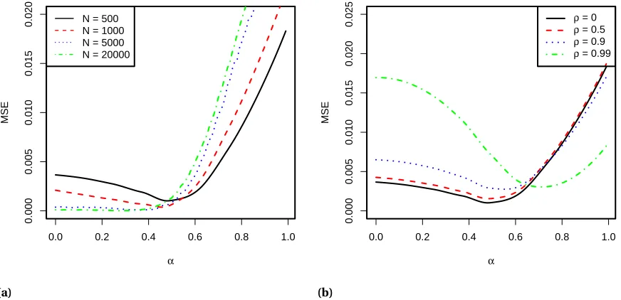
Figure 2.2 A normal distribution (d =2) with correlationρ, sample sizeN, andk=5 is
used to measure the efficiency (MSE) of the LNC estimator for various values
ofα. (a) Larger sample sizes shrink the optimal value ofα. (b) The optimalα
is dependent on the correlation coefficient of the reference distribution. The
difference is only present for large values of the correlation (ρ >0.9). Sample
size wasN =1000. . . 20
Figure 2.3 Estimated mutual information between correlated normal variables
esti-mated using KSG2, LNC, and LNN averaged over 100 independent
replica-tions. Sample size ofN=1000 withk=10 used for KSG2and LNC. LNC used
α1000,10,2=0.7053. Theρaxis is plotted logarithmically approachingρ=1
(whereI =∞). The samples ofX1andX2were centered and scaled before
estimation of mutual information. Error bars show±σˆ for each estimator. The
maximum observed standard deviations were 0.037 for KSG2, 0.049 for iLNC,
and 2.153 for LNN. KSG2performs well untilρ=0.9999 and then quickly hits
its limit ofψ(N)−ψ(k). LNC and LNN both maintain an accurate estimate of
mutual information through all values ofρconsidered here (0≤ρ≤1−10−11).
LNN shows high variability for largeρ. . . 22
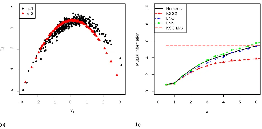
Figure 2.4 (a) Realizations of the banana distributions witha=1 anda=2 withb=1.
Changing the parametersa for the banana distribution affects the mutual
information between the random variablesY1andY2. Asaincreases the
dis-tribution concentrates on the parabola−b(Y12+a2). (b) Mutual Information
betweenY1andY2of the banana distribution. This shows that for non-normal
distributions the LNC and LNN algorithms outperform KSG2. . . 23
Figure 2.5 Realization of Sine Series Transformation. Variables(θ1,θ2,θ3)are AR(1) with
ρ1=−0.9 and(θ4,θ5)are AR(1) withρ2=0.7. (a) Pairwise plots of realizations
ofθ. (b) Realization of the mean process forθ= (0.58,−0.62, 1.06, 0.14, 0.01).
The parameterθ selects the amplitude of the frequencies chosen byγi j. . . 24
Figure 2.6 (a)d =30 case with 25 input dimensions and 5 outputs (k =60).Formula
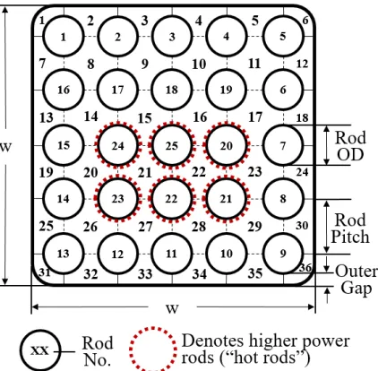
Figure 2.7 A cross-section of the 5×5 fuel rod bundle considered for the CTF calibration problem. Rods 20-25 were heated, all others were not. CTF calculates outlet temperature of the coolant for each subchannel. Because of the mixing be-tween subchannels the outlet temperatures are highly correlated bebe-tween neighboring subchannels. . . 27
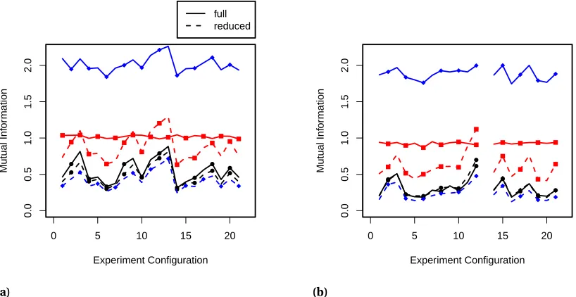
Figure 2.8 Mutual information estimates for each of the design configurations within
the pool of canidates for the CTF calibration problem. Solid lines indicate
the full (d=36) model and dashed lines indicate the reduced (d=3) model.
Mutual information is estimated usingN =1000 samples with KSG2(l), iLNC
(u), and LNN (n). (a) First stage of the design shows that configuration 13 is
the most informative point. (b) Second stage of the design (after sampling configuration 13) shows that configuration 12 is the next most informative point. LNN is the only estimator that shows benefit from the dimension reduction. . . 29
Figure 3.1 Minimize deterministic function f(x) =−2 cos(x)/(x2+1)using GP
optimiza-tion. (a) Interpolating GP from five sample points with a 95% credible band. (b) EI surface of GP whose maximum corresponds to the likely minimum of
f. Maximizing the EI function can be difficult because it is multimodal. . . 36
Figure 3.2 Diagnostics plots from
GADGET
for ALT example. EQI decreases and theesti-mated nugget effect stabilizes with increasing number of iterations. . . 40
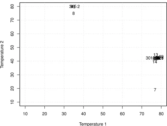
Figure 3.3 Location of each design within temperature space for each iteration of EQI. . 41
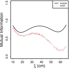
Figure 3.4 Steady State Heat Mutual Information. Mutual information between posterior
samples of the parameters and corresponding model predictions at each
design location (ξ). Sample size was fixed atN=5000. . . 42
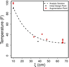
Figure 3.5 Ten points sequentially added to the three point initial design. . . 43
Figure 3.6 The resulting design places almost all of the points on the boundaries of the
design space. . . 44
Figure 4.1 Satellite image of the problem geometry, source location, and stationary
detector positions from Stefanescu et al.[2017]. . . 47
Figure 4.2 (a) Rayri−r0, segment lengthss1,s2,s3, and average cross-sectionsσ1,σ2,σ3
for gammas passing throughMi=3 buildings from a source atr0to theit h
detector atri. (b) Radiation attenuation due to theMi=3 buildings. . . 48
Figure 4.3 Kernel density estimate of the posterior source location for the five-minute
Figure 4.4 The average posterior source intensity plotted over the search domain for the five-minute dwell observations. Average source intensity is highest on the boundary of the search domain and lowest at points near the detectors. The region near the true source has average source intensity that is consistent
with the true intensity ofI0=3.214×10⁹cps. . . 53
Figure 4.5 A kernel density estimate of the source location posterior sampled based
on the sixty-minute dwell observations. With sufficient data the peripheral modes disappear and are replaced with a more concentrated bimodal distri-bution with maximum a posterior (MAP) estimate that is 4 meters from the true source. . . 54
Figure 4.6 An areal view of the ORNL search domain. Here we will focus on the first
experiment of[Hite et al., 2018]which involves the source labeled with “1"
and Group 1A and 1B detectors. . . 57
Figure 4.7 ORNL posteriors both zoomed out (a) and in (b). There is a bias between the
posterior sample and the source. The discrepancy of 6.66 m is on the same
order of magnitude as[Hite et al., 2018]. . . 58
Figure 4.8 Normal QQ-plot of the average estimated background parameters from the
ORNL data. The average background parameters are approximately normally
distributed except for the background estimates for detectors 1B-2 and 1B-3. 59
Figure 5.1 The circular area excluded by a simple hypothesis test with 0.9 power and 0.05
significance level for varying dwell times. As dwell time increases the exclusion area increases, but slows to linear growth for long dwell times. Detectors are good at measuring local radiation but as distance increases the corresponding dwell times have to increase as well. . . 63
Figure 5.2 Minimax designs for the localization problem forn=3, 4, 5, and 6 detectors. . 65
Figure 5.3 (a) A comparison of mutual information estimated from responses of the
fixed background and random background models. The line isy =x. There
is a small difference between the two models in terms of estimated mutual
information. Mutual information was estimated using KSG2withn=1000
and k =5. (b) A comparison between the estimated mutual information
and the minimum distance criterion for each of the set of detector-locations
for then=3 problem. The maximin design has lower mutual information
compared to the optimal design. The optimal design shies away from placing detectors on the boundary of the search domain. . . 66
Figure 5.4 Mutual information (KSG2) maximizing designs for localization. . . 67
Figure 5.5 Comparing of the efficiency of the detector placements in terms of posterior
entropy for a varying number of detectors. Mobile detectors are the most efficient method for reducing posterior entropy. . . 68
Figure 5.6 The posterior distribution after five minute dwell observations from the set
ofn=3 mutual information optimal detector locations. . . 69
Figure 5.7 The posterior distribution after a second set of five minute dwell observations
Figure 5.8 The continuously optimized detector locations when 3 detectors are deployed. The placements are similarly dispersed as those seen in the discrete case shown in Figure 5.4a. Because we do not enforce the restriction that detectors are placed outside of buildings the entire array is shifted to the right. For this configurations the estimated posterior entropy of the source parameters was 8.66, which is worse than the three detector configuration using discrete optimization shown in Figure 5.4(a). . . 71
Figure 6.1 Empirical cumulative D-efficiency of Neyer (solid), 3POD (dashed), DS-inform
(dotted), and DS-noninform (dotdash). (a)µ=8,σ=0.5; (b)µ=0,σ=1. . . . 83
Figure 6.2 Empirical cumulative D-efficiency of Neyer (solid), 3POD (dashed), DS-inform
(dotted), and DS-noninform (dot-dash). (a)µ=0,σ=2; (b)µ=0,σ=4. . . 84
Figure 6.3 Mutual information estimated using Monte Carlo with 10000 prior samples
and numerical integration. Monte Carlo estimate is adequate throughout the design space. . . 91
Figure 6.4 A realization of a sensitivity testing withN =25 shots. The true sensitivity
parameters areµ=500 andσ=30. For each sensitivity test method the initial
parameter guesses wereµg =0,µmin=−100,µmax=100, andσg =10. The
mutual information (MI) test methods were each given different prior onµ.
The normal prior was mean 0 with variance 1000. The Cauchy distribution had location parameter 0 and scale parameter 1000. The t-distribution had 10 degrees of freedom, mean 0, and scale parameter 1000. The prior distribution for the mutual information tests governs the early search behavior of the test. The Cauchy distribution produces exponential expansion like the Neyer method. The t-distribution produces linear expansion like the 3POD method. The normal distribution produces sub-linear expansion that is slower than either of the two standard methods. . . 93
Figure B.1 Univariate examples of KLE neighborhood withk=5. The distanceεx(i)is
the width of the neighborhood defined by the fifth nearest neighbor ofxi. . . . 114
Figure B.2 A KSG1neighborhood withk=5. The distance between the red dot and the
blue dot givesε/2. The max-norm square centered on the red dot of widthε
defines the jointZ neighborhood. The green squares are the points within
theX ε−neighborhood wherenx =14. The orange triangles are the points
within theY ε-neighborhood whereny =12. . . 117
Figure B.3 The two enlarged data circles define the distance length of the rectangle inX
CHAPTER
1
INTRODUCTION
Computer simulations are a fundamental scientific tool for the study of nature. With the development
of computational resources and algorithms, high-fidelity simulations that nearly reproduce reality
in silicoaugment physical experimentation. Whether the simulations model nuclear reactors, the
spread of an epidemic, or the evolution of the planet’s climate, these simulations significantly
expand the realms of inquiry available to a traditional laboratory.
The design of computer experiments developed from the need to efficiently evaluate,
vali-date, and approximate these large simulation codes that can take days or weeks to run. Computer
experiments focus primarily on the exploration of deterministic simulations and heavily utilize space-filling designs. Such designs facilitate numerical integration, sensitivity analysis, parameter
subset selection, and the fitting of surrogate models to the computer simulation[Morris & Moore,
2015].
The design of computer experiments returns to its origins in the design of physical experiments
when considering the optimal calibration of computer simulations. Calibration is the process of
using physical data to select optimal parameter values and quantify their uncertainty to match a simulation’s output. The design problem that arises is choosing where in the design space to collect
data to produce best parameter inferences. However, because many of these simulation models are nonlinear with respect to their parameters and without analytic expressions, classical optimal
design theory falls short in providing robust optimal designs.
nuclear reactors where, due to legal, ethical, and financial reasons, full-scale physical experiments
are often scarce, and even the few data that are available must be used to calibrate and inform an array of multi-physics simulations required to simulate a critical reactor core. Any increase in the
efficiency of the experimental design contributes to safer and more efficient nuclear reactor designs.
Because many of the processes within a reactor core are nonlinear, designing an experiment to collect calibration data suffers from the fundamental problem in optimal nonlinear experimental
design where the optimal design is dependent on the unknown model parameters. The popular
remedies to these difficulties are sequential and Bayesian experimental design. Sequential designs take small steps (experimental unit allocation), slowly accumulating empirical information that
refines the experimental design for more efficiency throughout the experiment. Bayesian
experi-mental design instead relies on prior information to constrain the optimal design. Such designs are called average, agglomerated, or compromise designs because they weight designs that are optimal
for particular parameter values according to their prior weight. Although they may reduce efficiency
for any potential parameter value, they are hopefully robust to parameter uncertainty.
We present contributions to the unity of sequential and Bayesian experimental to improve
design efficiency for small sample experiments. We take a simulation-based approach where the
design criterion is estimated through model sampling. Mutual information is the design criterion we use through our work, optimized using noisy Gaussian process optimization. We apply this to
applications in the calibration of thermo-hydraulic codes, mobile radiation detector placement, and sensitivity testing of detonators.
1.1
Optimal Nonlinear Design
The design of experiments (DOE) for linear models is a mature field. Mathematically, it is convenient
to describe an experimental design as a probability measureηon a design spaceX, whereξ∈ X
denotes the factor-levels for a single experimental unit. A designηthat can be carried out on a
finite set of experimental units is called anexactdesign. Often,ηis anapproximatedesign, which
is a relaxation of exact designs that allows for fractional experimental units. The discretization
(rounding) of an approximate design is a nontrivial problem[Pukelsheim & Rieder, 1992].
Optimal experimental design attempts to gain the most information for a fixed amount of resources and provide the best inference for the quantities of interest. Because the Fisher information
matrix determines the asymptotic variances of the maximum likelihood estimators (MLE), it has
been the focus for measuring the quality of a design. Ideally, a design would minimize the variances
of every function of the parameters, but this is impossible[Silvey, 1980, pp. 4-5]. Instead, designs are
found that maximize a particular function of the information matrix,φ, called a design criterion.
Each criterion is measuring the “size" of the information matrix in different ways that lead to designs
The Fisher information matrix for approximate designηis defined asM(η) =E[ξξT]whereξis
anηdistributed random vector. Two major types of designs for linear models are D-optimal and
G-optimal designs. D-G-optimal designs maximizeφD(η) =log det(M(η)). Maximizing the determinant
of the information matrix maximizes the power of the model F-test. G-optimal designs minimize
φG(η) =sup λTM(η)−1λ, which minimizes the maximum variance over all linear functions of the
model parameters (minimax). Designs for linear models are often geometrically intuitive, such as
spreading design points out and maintaining symmetry[Elfving, 1952].
A significant series of results in optimal experimental designs are the numerous equivalence
theorems. The first is Kiefer & Wolfowitz[1960]who proved that for linear models D-optimal designs
and G-optimal designs are equivalent. The General Equivalence Theorem (GET) from Whittle[1973]
enumerated equivalent conditions for a design to beφ-optimal whenφis a concave function with
Fréchet derivatives. The Fréchet derivative
F(η1,η2) = lim
α→0+
φ((1−α)η1+αη2)−φ(η1)
α ,
is the directional derivative ofφatη1in the direction of designη2. The GET provides conditions to
verify a proposed design’s optimality.
Theorem 1.1(General Equivalence Theorem). Ifφis a concave function of design measureηand
ηξis design supported on the single pointξ, then the following statements are equivalent:
1. η?maximizesφ(η)
2. η?minimizes supξ∈ΞF(η,ηξ)
3. supξ∈ΞF(η?,ηξ)≤0
For nonlinear models, Theorem 1.1 becomes more complicated because the Fisher information
matrix is often dependent on the unknown model parametersθ[Silvey, 1980, p. 53]. We write the
design criterion asφθ(η) =φ(η,θ)to emphasize the dependence onθ. The linear model case is
unique because there is singleφθ-optimal design for all parameter values. Even with the dependence
onθ, the GET holds for nonlinear models under mild regularity conditions[Dubov, 1977]. A design
that isφθ-optimal is called alocally-optimaldesign. The simplest solution to the dependence on
model parameters is to assume a nominal value for the model parameters and use a locally-optimal design. If the designer has a reasonable initial estimate of the model parameters, then a local design
will be efficient[Ford et al., 1989].
Sequential locally optimal designs are a standard solution to nonlinear design problems. Al-though not strictly optimal, by iteratively estimating the model parameters and updating the locally
optimal design with improved parameter estimates, the design converges to the true locally
D-optimal designs for estimation of nonlinear models. The drawbacks of sequential designs are
their logistic difficulties and their need to analyze new data throughout the experiment, which may be computationally costly.
1.2
Bayesian Design
A fundamental tenet of experimental design is leveraging prior knowledge to produce better designs. A classic example is the incorporation of restricted randomizations like split-plot, block, and Latin
cube designs that account for anticipated variation between experimental units or strata. The dependence of nonlinear designs on model parameters lends itself to the use of prior belief as in
Bayesian statistics.
The Bayesian experimental design problem was mathematically described by Lindley[1972]by
focusing on the expected utility of designη
Λ(η) = Z Z
u(η,θ,y)p(y|θ,η)p(θ)d y dθ, (1.1)
whereuis the utility being used andp(θ)is the experimenter’s prior distribution for the parameter
θ. The optimal Bayesian design is thenη? =argmaxΛ(η), where the parameter uncertainty is
marginalized. The Bayesian D-optimality criterion is
ΛD(η) = Z Z
log det(M(η,θ))p(y|θ,η)p(θ)d y dθ. (1.2)
The optimal design maximizes the expected log determinant with respect to the prior distribution,
making the design robust to incorrect guesses of the parameters[Chaloner & Verdinelli, 1995].
The simple case of Bayesian linear regression with conjugate priors is similar to those discussed in
Section 1.1. The inverse posterior covariance matrix[M(η)−1+R]−1, whereRis the prior covariance
matrix of the parameterθ, replaces the Fisher information matrix, and the familiar D or G-optimal
criteria are applied. The prior information contained inR may constrain the design by informing
the design about known correlations between parameters. Chaloner[1984]extended the GET to the
Bayesian regression case.
Numerous technical issues arise in Bayesian design. For example, because the design criterion
(1.1) is generally not a function of a positive-definite matrix, the Carthéodory theorem does not
guarantee that there exists an optimal design supported by a finite number of design points[Ford
et al., 1992]. Chaloner & Larntz[1989]demonstrated this feature for the logistic model, showing that
the number of design points increases when the prior distribution becomes more diffuse. For some
prior distributions there is no global D-optimal design, which causes (1.1) to be non-concave[Firth
In general, the computation of (1.1) is difficult except for the simplest models. One tactic is to
separate the Bayesian design into two pieces: a design phase and an inference phase[Tsutakawa,
1972]. A prior in the design phase could be selected for its tractability, whereas the final analysis
uses a noninformative prior. For example, approximating the posterior distribution with a normal
distribution will simplify the computation of (1.1). By simplifying the computation, the expected
utility is optimized in a brute-force manner using Nelder-Mead[Chaloner & Larntz, 1989]or
point-exchange[Zhang & Meeker, 2006]algorithms. Gotwalt et al.[2009]developed an efficient numerical
integration method to compute the D-optimality criterion for cases when the prior is a multivariate normal distribution.
Monte Carlo integration could be used to compute (1.1) with parameters sampled from the prior
ofθ. Estimating the expected utility using Monte Carlo makes (1.1) an expensive, noisy optimization.
The need to use simulations to compute and optimize (1.1) has produced many techniques in
simulation-based design discussed in the next section.
1.3
Simulation-Based Design
Computational difficulty often stifles the appeal of Bayesian design. The fundamental design
prob-lem divides into two parts: estimation and optimization of (1.1). The challenge of estimating and optimizing a design criterion for a particular parameter distribution has spurred the development
of various approximations in the literature[Ryan et al., 2015].
Discretizing the parameter prior makes the design criterion computation tractable[Woods
et al., 2006]. The resulting estimator weights the designs according to a finite collection of potential
parameters, producing an average of locally optimal designs. Given the criterion and a candidate set
of design points, an exchange algorithm computes exact designs[Fedorov, 1972; Cook & Nachtsheim,
1980]. Alternatively, the averaging of designs could be performed by clustering points from a pool of
locally optimal designs[Dror & Steinberg, 2008].
For non-classical design criteria, it may be difficult to apply a direct estimate of the criterion as discussed above. This is because for Fisher Information matrix methods the matrix is a linear
combination of the individual information matrices. The full utility expression in (1.1) is dependent
on the data observed, so it is dependent on the likelihood function or conditional distribution of the data. Instead of a single integral in (1.1) a double integral must be computed over the parameters
and the potential data. The integral is computational costly if double Monte Carlo estimates, see
Algorithm 1.1, are required.
A simulation-based design approach is one method for overcoming these problems. This
ap-proach involves the simulation of model output and the use of that information to make the best estimate of where to collect data for subsequent runs of the experiment. In a sense, the
Algorithm 1.1Monte Carlo Estimator ofΛ
Require: η,A,B
fori=1, ...,Ado
sampleθi∼π(θ)
sample yi∼π(y|θi,η)
for j=1, ...,Bdo
sampleθj ∼π(θ|yi)
uj =u(η,θj,yi)
end for
ui=B1PB i=1uj
end for returnA1PA
i=1u i
to the previously discussed method, the simulation-based experimental design is quite general
because no analytic expressions are needed to find the optimal design. One only needs to simulate
posterior distributions and predictive values from the model[Solonen et al., 2012; Liepe et al., 2013;
Huan & Marzouk, 2013].
With an estimate of the design criterion, a type of stochastic optimization must be applied. The
estimated criterion can be optimized directly using an augment-probability model[Müller, 2005],
genetic algorithm[Hamada et al., 2001], or simulated annealing[Solonen et al., 2012]. Alternatively, a
surrogate or response surface can be fit to the observed points on the criterion surface and optimized
instead. Müller & Parmigiani[1995]used a polynomial response surface. Huan & Marzouk[2013]
use polynomial chaos model. Weaver et al.[2016]and Overstall & Woods[2017]employed Gaussian
processes as surrogates.
1.4
Overview
The present work contributes to the field of optimal sequential Bayesian experimental designs by advancing the tools for computing these designs. We develop mutual information estimators
and software to compute optimal designs. We apply Bayesian design to three applications:
high-to-low fidelity model calibration of thermo-hydraulic codes in nuclear reactor simulations, the sensitivity testing of explosive detonators, and the adaptive placement of radiation detectors for
source localization. We outline the work completed in the following subsections.
1.4.1 Evaluating Mutual Information Estimators for Experimental Design
and potential observations is computationally intractable without using normal approximations
or Monte Carlo estimates. Recent work has utilized nonparametric k-Nearest Neighbor (kNN) estimators to select near-optimal experimental runs. Here we explore the efficacy of current kNN
estimators in experimental design applications. We demonstrate that although kNN estimators
are biased estimators of mutual information, they are still applicable to making design decisions in moderately high dimensions. Finally, we present a modified kNN estimator that has lower bias
than current kNN estimators with improved tuning parameter calibration. The kNN estimators
developed in this research have been released in theRpackage
rmi
, which is available on CRAN(Comprehensive R Archive Network -
https://cran.r-project.org/
).We apply kNN estimators to the problem of high-to-low fidelity calibration in nuclear reactor
subchannel codes. The high-to-low calibration is often used in Uncertainty Quantification when
fitting surrogate or simplified models to computationally expensive simulations[Kapoor et al., 2007]
and specifically in nuclear reactor applications[Raza & Kim, 2008]. We look at the subchannel
code COBRA-TF, which does not have a closed form expression and therefore classical optimal design results cannot be directly applied. Utilizing kNN estimators we use a simulation-based design
approach that approximates an optimal design for sampling the high fidelity, computational fluid
dynamics, code STAR-CCM+for the calibration of COBRA-TF.
1.4.2 Gaussian Process Approximations for Designing Experiments
Weaver et al.[2016]used Gaussian process optimization, a form of Bayesian optimization, to compute
optimal Bayesian design of experiments. Their algorithm approximates the experiment’s design criterion surface using a Gaussian process and then iteratively employ the Expected Quantile
Improvement (EQI) acquisition function[Picheny et al., 2013]to optimize the criterion. EQI is a
generalization of the Expected Improvement (EI) acquisition function used in the Efficient Global
Optimization (EGO) algorithm[Jones et al., 1998]to stochastic objective functions.
We developed the Gaussian process Approximations for Designing ExperimenTs (
GADGET
)R-package that implements the methods of Weaver et al.[2016].
GADGET
includes batch, sequential, orbatch-sequential designs for both physical and computer experiments. Finally,
GADGET
computesdiagnostic statistics on the Gaussian process optimization to detect lack-of-fit of the surrogates
during the optimization to prevent sub-optimal designs from being chosen. We apply
GADGET
to thethree design problems: the accelerated life testing (ALT) from[Weaver et al., 2016], the steady-state
heat diffusion example from[Lewis et al., 2016], and the crystallography binary regression example
1.4.3 A Bayesian Hierarchical Model for Background Radiation
A fundamental challenge in estimating the location of a missing radioactive source from detector observations is the presence of background radiation. This non-source radiation is caused by
radioactive decay of naturally occurring radioactive materials (NORM) in the ground or buildings
and cosmic sources. The effect of background varies within both space and time at different scales. Current approaches to Bayesian source localization assume that background radiation is constant
across the entire problem domain, an assumption that is untenable with increasing stand-off
distances from the source.
We consider an urban radioactive source localization problem in the presence of background
radiation. We propose a hierarchical Bayesian model that simultaneously infers the source
loca-tion and the rate of background radialoca-tion at each detector localoca-tion without the requirement of separate calibration. We employ a simplified photon transport model to reduce the computational
requirements of Bayesian model calibration. We demonstrate the model’s accuracy by localizing a Cesium-137 source in a simulated block in Washington D.C., and we analyze experimental field
observations with background noise taken at Oak Ridge National Laboratory (ORNL). In both
cases, we demonstrate that the model provides sufficient fidelity that we can isolate a source while simultaneously estimating background radiation.
1.4.4 Radiation Localization using Mobile Detectors
We consider the problem of mobile placement of radiation detectors in an urban source localization
problem. Based on the work done in estimating background radiation, the efficiency of radiation detectors to localize a source decreases with longer dwell times. We gain a significant increase in
efficiency by moving detectors closer to the suspected location of the source. We frame the mobile
placement strategy as a sequential Bayesian experimental design problem.
We continue the work of Schmidt[2016]for the placement of radiation detectors on a discrete grid
of potential detector locations. We demonstrate that sequentially adapting the detector locations based on an initial set of detector observations reduces the observed posterior entropy of the source
location. We see that movement of detectors is more efficient than deploying more detectors in the
problem domain.
Finally, we consider a continuous detector placement analog to the problem formulated by
Schmidt[2016]. We utilize the Gaussian process optimization technique available in the
GADGET
pack-age. We find that standard kNN mutual information estimators cannot be reliably used in conjunc-tion with Gaussian process optimizaconjunc-tion, but our higher fidelity mutual informaconjunc-tion estimator
developed in Chapter 2 is capable of producing optimal continuous detector placements using
1.4.5 Mutual Information Sensitivity Testing
Explosives detonate, either intentionally or accidentally, when exposed to a sufficiently large physical shock, heat, or electrostatic discharge. Sensitivity testing is an experimental procedure used to assess
the safety and reliability of explosives, detonators, and other energetics. The goal is to estimate
what stimulus level will guarantee the detonation of a certain percentage of samples. Sensitivity testing is closely related to dose-response experiments in clinical trials. Sensitivity testing involves
the sequential selection of stimuli and observation of whether detonation occurs or not.
Stochastic approximation algorithms have dominated sensitivity testing since the 1940s because
they are easily carried out without a computer[Dror & Steinberg, 2008]. The sensitivity model is a
generalized linear model (GLM), which makes sensitivity testing a nonlinear design problem. The
current best methods implement a hybrid algorithm that incorporates a stochastic search across various stimulus levels until maximum likelihood estimates (MLE) can be computed, after which
stimulus levels are chosen sequentially to optimize the D-optimality criterion centered at those
estimates, a sequential local D-optimal approach[Neyer, 1994; Wu & Tian, 2014]. We review the
state-of-the-art methods for designing sensitivity tests and compare their efficiencies. Asymptotically all
sequential D-optimal designs produce the same continuous designs. The differences occur during the initial heuristic search phases used to establish MLEs. When sample sizes are small, it is likely
that the initial search phase comprises a sizeable proportion of the total sample size yet is not
optimized for the inference of the model parameters. We present preliminary work that attempts to quantify the differences of the heuristic search phases of sensitivity test algorithms theoretically by
recasting each algorithm as an equivalent sequential Bayesian experimental design. The equivalent
Bayesian designs elucidate the assumed prior knowledge and likelihood used in each algorithm. By better understanding these search phases it may be possible to increase the efficiency of small
CHAPTER
2
EVALUATING MUTUAL INFORMATION
ESTIMATORS FOR EXPERIMENTAL
DESIGN
2.1
Introduction
Computer model calibration involves inferring the model parameters of a computer code to produce a more accurate representation of the physical system it depicts. Ideally, model calibration utilizes
accurately collected data, but due to cost or feasibility the available data may be insufficient for
cali-bration. A possible solution is to use validated high resolution simulations –here called high-fidelity codes– to simulate data for calibrating a low-fidelity code, which we call high-to-low calibration.
Beyond the strict sense of selecting optimal parameters for the low-fidelity model, calibration also
applies to the more general case of improving the low-fidelity model, possibly correcting systematic model discrepancies.
Our motivating problem for high-to-low calibration is the calibration of the nuclear reactor code
COBRA-TF (CTF). CTF is a subchannel code that models the thermo-hydraulics within a reactor core
and is used to evaluate reactor safety[Salko & Avramova, 2015]. CTF computes state averages along
CIPS (CRUD Induced Power Shift) that are affected by local flows. In comparison, the high-fidelity
code STAR-CCM+, a computational fluid dynamics (CFD) code, can resolve these local features, but
with a significant increase in computational cost. For example, a CTF 5×5 rod bundle simulation
takes 5 minutes on a single processor whereas the same problem takes 1 hour on a 1000 core cluster
with STAR-CCM+ [Gilkey, 2017]. The high computational cost of STAR-CCM+prevents its use in
uncertainty quantification. By calibrating CTF to STAR-CCM+, more accurate, spatially varying,
mixing parameters could be obtained, allowing CTF to incorporate the effects of turbulence within
the reactor core and reduce the operating uncertainty of a reactor.
Lewis et al.[2016]proposed a simulation-based Bayesian framework for high-to-low calibration
using mutual information to determine the most informative high-fidelity runs for the low-fidelity
calibration. Simulation-based design methods utilize draws from parameter distributions and
for-ward model evaluations to determine the most informative experimental design[Müller, 2005].
Simulation-based design is a “black-box” experimental design method where the model is
in-terrogated repeatedly to determine the optimal design. Typically these simulation-based design algorithms incorporate a stochastic estimate of the expected utility of a proposed design and an
optimization algorithm to find the optimal design. Monte Carlo estimates of an expected utility are
often used[Solonen et al., 2012; Liepe et al., 2013; Huan & Marzouk, 2013]as well as importance
sampling[Berg et al., 2003]. Müller[2005]uses a stochastic Monte Carlo design criterion for the
design problem and optimizes the criterion using MCMC applied to an augmented probability model.
Mutual information, or expected information gain, is a common criterion for simulation-based
design[Drovandi et al., 2013; Ryan et al., 2016]. Mutual information is an information theoretic
quantity that measures the dependence between two random variables by quantifying the amount
of information in terms of Shannon entropy that knowledge of one variable provides about the other
and has been used in experimental design for decades[Lindley, 1956]. In the context of Bayesian
model calibration, mutual information is the expected Kullback-Leibler divergence between the
prior and posterior distributions of the calibration parameters. Maximizing mutual information
is a generalization of Bayesian D-optimality for linear models with Gaussian error[Chaloner &
Verdinelli, 1995]. Mutual information measures how informative high-fidelity observations will be
for the low-fidelity model regardless of the complexity of the low-fidelity model.
Mutual information is difficult to compute, and analytical formulas principally exist only for lin-ear models with normally distributed errors. Fortunately, because mutual information is a general
measure of dependence between random variables, it is used in many fields outside of
experi-mental design, including variable selection[Doquire & Verleysen, 2012; Vergara & Estévez, 2014],
independent component analysis[Stögbauer et al., 2004], signal processing[Achard et al., 2005],
genetics[Steuer et al., 2002], clustering[Kraskov et al., 2005; Steeg et al., 2014], and machine learning
the development of a wide range of estimators: Monte Carlo[Chávez & Henrion, 1994; Müller &
Parmigiani, 1995], Histogram/Binning[Fraser & Swinney, 1986; Paninski, 2003], Edgeworth series
[Hyvärinen, 1998], k-Nearest Neighbor (kNN)[Kraskov et al., 2004], and kernel density estimate
(KDE)[Moon et al., 1995].
Terejanu et al.[2012]and Lewis et al.[2016]both used the nonparameteric
Kraskov-Stögbauer-Grassberger (KSG) estimator of Kraskov et al.[2004]to estimate mutual information from model
samples and maximized KSG over a discrete set of potential designs. The KSG estimator was
devel-oped for independent component analysis with the goal of empirically testing for independence,
whereas experimental design requires finding dependence. Furthermore, Gao et al.[2015a]
demon-strated that KSG has a maximum estimable mutual information for a given sample size, a feature
that affects histogram-based estimators as well[Kannan & Tegnèr, 2014; Zheng & Benjamini, 2016]. If
two design configurations have mutual information higher than this threshold there is no guarantee
that KSG is able to differentiate between the configurations.
There are alternative kNN mutual information estimators to KSG that are less biased. Gao
et al.[2015a]and Lord et al.[2018]use empirical volume estimates with KSG and have shown
much lower bias when applied to highly dependent relationships. Other estimators utilize local
Gaussian likelihood estimates with kNN-tuned bandwidths, which also have lower bias and proven
consistency[Gao et al., 2015b; Gao et al., 2017]. Both of these classes of estimators correct for
observed correlations within the sampled data and extend the estimation of mutual information to regimes of higher dependence without increasing sample size, but with the introduction of difficult
to select tuning parameters. It remains to be demonstrated that these improved estimators are more
effective in experimental design applications.
Another obstacle for estimating mutual information in experimental design is the high
dimen-sionality caused by the large number of parameters and model responses in design problems. For
example, the CTF calibration problem we consider has 36 responses; 1 for each subchannel outlet temperature. Moreover, if multiple design configurations are selected at each iteration, the number
of responses increases multiplicatively. Similar high dimension problems occur in image processing
where mutual information is calculated between vectors of pixels[Kybic & Vnuˇcko, 2012]. The major
focus of mutual information estimation has been on the two dimensional case with a few exceptions.
Kraskov et al.[2004]used an 8-D multivariate as an example and Gao et al.[2015a]used 5-D linear
and 5-D quadratic functions as synthetic examples.
A pragmatic solution to the problem of high dimensional estimation of mutual information is to
perform dimension reduction before estimating mutual information. For example, Lin et al.[2019]
used canonical correlation analysis (CCA), which produces two 1-D random variables that have the highest correlation, and computed mutual information using KSG on the dimension reduced
samples. Lin et al.[2019]then use the information processing inequality to show that this produces a
whether dimension reduction, which must be applied separately for each design configuration,
preserves comparisons of estimated mutual information between configurations.
Here we investigate the efficacy of the kNN mutual information estimators for experimental
design applications. We propose an improved version of the mutual information estimator of
Gao et al.[2015a]that computes high dimensional information gain instead of high dimensional
redundancy and present a new method for tuning its calibration parameters. In addition to simulated
examples, we consider the problem of using kNN estimators to select design configurations for the
calibration of the subchannel code COBRA-TF (CTF) with and without dimension reduction. We found that KSG is sufficiently accurate for choosing maximally informative design configurations.
Due to its severe bias, it is an estimator of nominal mutual information. Our proposed estimator
is shown to be less biased than KSG and better suited for experimental design in certain high dimensional cases.
2.2
Design
Letd`(θ,ξ)denote the low-fidelity model, which is a function of calibration parametersθ∈Rp and
configuration or design variablesξ∈Ξ. HereΞdescribes the set of possible design points of the
configuration variables. We calibrate this low-fidelity model using data obtained from a high-fidelity
modeldh(ξ). Letξnbe the design point corresponding to thenthhigh-fidelity observation ˜dngiven
by
˜
dn=dh(ξn) +"˜n(ξn),
where ˜"n(ξn)denotes the error in observing the high-fidelity code atξn, which may not be normally
distributed. We relate the low-fidelity model to the high-fidelity observations using the statistical
model from Kennedy & O’Hagan[2001],
dh(ξn) =d`(θ,ξn) +δ(ξn) +"n(ξn). (2.1)
Here we denote potential additive discrepancy in the low-fidelity model byδ(ξn)and random
observation or discretization errors by"n(ξn).
Given a set of observationsDn−1={d˜1, ˜d2, ..., ˜dn−1}of the high-fidelity code, we seek a design
pointξnso that uncertainty in the low-fidelity calibration parametersθis reduced when the model
is re-calibrated using the new high-fidelity data point ˜dn. The change in knowledge about the model
parameters, due to the addition of new data ˜dn, is given by Bayes’ rule
p(θ|Dn) =
p(Dn|θ)p(θ) p(Dn) =
for the new data setDn={d˜n,Dn−1}. Because our objective is to determine the distribution of the
parametersθfrom the calibration of our low-fidelity model with data ˜dn, using as few experiments
as possible, the strategy upon which we base our design decision should be chosen according to
the amount of information provided by the proposed data as a result of measuringdh(ξn)atξn.
Because ˜dnhas not yet been observed before choosingξn, we employ predictionsdnprovided by
the statistical model (2.1) to determineξn. As detailed in Lewis et al.[2016], the optimal design
conditionξ∗nmaximizes the mutual information
I(θ;dn|Dn−1,ξn) = Z
D Z
Ω
p(θ,dn|Dn−1,ξn)log
p(θ,dn|Dn−1,ξn) p(θ|Dn−1)p(dn|Dn−1,ξn)
dθd dn; (2.2)
that is,
ξ∗
n=arg maxξ
n∈Ξ
I(θ;dn|Dn−1,ξn). (2.3)
The high-fidelity code is then evaluated using the design conditionξ∗n and the resulting data ˜dn
is used to re-calibrate the model parametersθ. Instead of computing mutual information (2.2)
analytically or numerically, Lewis et al.[2016]estimated mutual information on a grid of points
within the design space using the KSG estimator[Kraskov et al., 2004], and optimization (2.3) was
performed by takingξn that maximized the observed estimate of mutual information. Because
design points are chosen to maximize the information in the next design steps, this is a greedy sequential search strategy for an optimal design, but the framework can be extended to selection
of batches{dn,dn+1, . . . ,dn+b−1}, b >1 for non-myopic batch-sequential design. The sequential
search is continued until either a predetermined number of high-fidelity runs are performed or until the estimated mutual information for all remaining design points is below a chosen threshold
[Adams et al., 2018, p. 67]. The quality of the design obtained using this procedure is determined by
the quality of the mutual information estimator.
2.3
Mutual Information Estimators
The mutual information between calibration parametersθand lower-fidelity predictionsdncan be
decomposed as
I(θ;dn|Dn,ξn) =H(θ|Dn,ξn) +H(dn|Dn,ξn)−H(θ,dn|Dn,ξn), (2.4)
whereH(X)denotes the Shannon differential entropy of random variableX. For brevity, we drop
the explicit conditioning on the previous dataDnand design pointξn, except in cases where it is
2.3.1 Kraskov-Stögbauer-Grassberger (KSG) Estimators
Kraskov et al.[2004]utilizes the decomposition (2.4) and the Kozachenko-Leonenko entropy (KLE)
estimator[Kozachenko & Leonenko, 1987; Singh et al., 2003]. The KLE estimator estimates the
entropy of a random variableX from a sample of sizeN by computing the distance between theith
sample point and itskthnearest neighbor, denotedε
x(i)/2. The KLE estimator is
ˆ
HKLE(X) =ψ(N)−ψ(k) +log(cdx) +dx N
N X i=1
logεx(i). (2.5)
Heredxis the dimension of the observations andcdx is the volume of the unit ball inR
dx for the
metric used to measure the distance between nearest neighbors, andψ(·)is the digamma function.
The assumption made in the derivation of KLE is that the density ofX is well-approximated by a
uniform distribution within the neighborhood that contains the pointxiand itsk nearest neighbors.
Singh et al.[2003]proved the KLE estimator is consistent for 1≤k <N under the added assumption
thatX is absolutely continuous and showed through simulation thatk ∈ {3, 4, 5, 6}minimized the
estimator’s root-mean-square error (RMSE). Utilizing the KLE estimator and the mutual information decomposition (2.4) gives a plug-in estimate of mutual information.
Kraskov et al.[2004]identified that the plug-in estimator of mutual information based on KLE
would suffer from bias due to the accumulation of errors in computing the neighbor distances
within the joint and marginal spaces. Kraskov et al.[2004]proposed two estimators that eliminate
this bias by forcing the cancellation of the distance terms in (2.5). They achieved this by fixing an
εdistance in the joint space and using it in the marginal spaces. Because the nearest neighbor
distance is fixed, thek used in the marginal spaces is allowed to vary point-wise.
Letzi= (xi,yi)andzik= (xik,yik)be thekthnearest neighbor of pointziin the joint space ofXand
Y. The first estimator proposed in Kraskov et al.[2004], denoted by KSG1, defines a neighborhood
radius for pointi asε(i)/2=||zik −zi||∞. Thisε(i)is then assumed for each of the marginals to
computenxi(ε(i))andnyi(ε(i)), which are the number of sample points covered in the marginal
space by the interval centered atziwith widthε(i). Formally, these are defined as
nxi(ε(i)) =
X j6=i I
||xj−xi||∞< ε(i)
2
andnyi(ε(i)) =
X j6=i
I
||yj−yi||∞< ε(i)
2
. (2.6)
Utilizingnx(ε(i))andny(ε(i))as the appropriate neighbor orders for theX andY marginals for
each point in the KLE estimator and substitution into (2.4) yields
KSG1(X;Y) =ψ(N) +ψ(k)− 1
N N X i=1
ψ(nx(ε(i)) +1)− 1
N N X i=1
A drawback of KSG1is that the KLE estimator is only used correctly in one marginal space because
the distance to thekthnearest neighbor in the joint space will correspond to thekthnearest neighbor
distance in one of the marginal spaces. Independently scaling each variable to unit standard
devia-tion often eliminates any discrepancies caused by this imbalance. However, scaling may not prevent
bias in KSG1if the variables exhibit heteroskedasticity. The second KSG estimator follows the same
argument as the first but utilizes a modified version of the KLE estimator that is generalized from a
square to rectangular neighborhood. This allows the estimator to adapt to the heteroskedasticity of
the sample point-wise. As with KSG1, the set of nearest neighbors is determined by distances within
the joint space, but marginal distancesεx(i)andεy(i)are computed in each of the marginal spaces
separately as
εx(i)
2 =1≤maxj≤k||x
j
i −xi||∞and εy(i)
2 =1≤maxj≤k||y
j
i −yi||∞.
The marginal orders are computed as
nx(εx(i)) = N X
j=1 I
||xj−xi||∞≤ εx(i)
2
andny(εy(i)) =
N X
j=1 I
||yj−yi||∞≤ εy(i)
2
.
The estimator is then
KSG2(X;Y) =ψ(N) +ψ(k)− 1
N N X
i=1
ψ(nx(εx(i)))− 1
N N X i=1
ψ(ny(εy(i)))−1
k,
where the extra 1/k term comes from transitioning to rectangular areas in the joint space entropy
estimate.
KSG estimators have one serious flaw: they can only estimate a maximum mutual information
of approximatelyψ(N)−ψ(k)for a fixed sample sizeN and orderk. Gao et al.[2015a]proved that
both KSG estimators suffer from this effect and, because the digamma functionψ(N)grows
loga-rithmically, the sample size needed to estimate mutual information increases at least exponentially in mutual information. This upper limit to estimable mutual information is not an issue if the goal
is to find independence between samples[Stögbauer et al., 2004]or to simply look for dependent
relationships[Reshef et al., 2011]. But because experimental design requires maximizing mutual
information, the mutual information estimators may not identify the true maximum. Moreover,
because mutual information is not knowna priori, it is difficult to set the needed sample size for
2.3.2 Improved Local Neighborhood Corrected KSG Estimator (iLNC)
The critical assumption of KSG estimators is that the joint density is uniform within the neighbor-hood of every sample point, which is violated in small sample sizes drawn from highly dependent
random variables. Gao et al.[2015a]proposed a modified KSG algorithm, the Local Neighborhood
Corrected (LNC) KSG estimator, that adjusts for local non-uniformity by modifying the local support of the joint density by computing the volume of each point’s neighborhood using a principal
com-ponent analysis (PCA) aligned rectangle instead of KSG’s axis-aligned volume. This modification
does not remove the local uniformity assumption, but shifts the domain in which it holds[Singh &
Póczos, 2016]. The LNC estimator is derived by expressing KSG2as a sample average,
KSG2(X;Y) = 1
N N X i=1
logPzi(εzi)
Vzi(εzi)−log
Pxi(εxi) Vxi(εxi)−log
Pyi(εyi)
Vyi(εyi)
wherePw(ε)is the number of points within theε/2 ball centered atw andVwis the volume of the
ε/2 ball centered atw. This formulation makes it clear that KSG2is estimating the joint and marginal
densities at each point within the sample. LNC swapsVzi with ¯Vzi, the PCA-aligned volume of the
neighborhood, computed by taking the singular-value decomposition (SVD) of the neighborhood
matrix. Because of the logarithm it is then easy to express LNC as KSG2with an additive correction,
LNC(X;Y) =KSG2(X;Y)− 1
N N X i=1 I
¯ Vzi
Vzi
< αk,d
log ¯
Vzi
Vzi
. (2.7)
The correction term in (2.7) includes a threshold indicator function to filter out spurious
non-uniformity corrections. By random chance, the PCA volume will often be smaller than the
axis-aligned volume even when the local uniformity assumption holds. The threshold is set with a tuning
parameterαk,dthat depends on both the dimension of joint spacedand neighborhood orderk.
Recent work by Lord et al.[2018]modified the KLE estimator in a similar fashion as LNC to
produce an improved mutual information estimator. Instead of using PCA, they estimate the local support with ellipsoids to provide a tighter fit around the neighborhood. The performance of their
estimate was similar to LNC for small sample sizes, but showed an asymptotic bias in large sample
sizes, which is probably caused by their estimator’s lack of a threshold for applying corrections as
in LNC. An advantage of the estimator by Lord et al.[2018]is that, because KSG was not used as a
foundation, their corrections were applied to both the marginal and joint spaces separately, whereas
LNC only has a correction for the joint space. The application of marginal corrections is important when the marginals are multidimensional, which is the case in experimental design applications.
Gao et al.[2015a]generalized LNC to multivariate mutual information by computingredundancy,
![Figure 2.1 The solid lines are estimated α from Gao et al. [2015a] and dashed lines are our MSE minimiz-ing α for d = 2,3,5,10](https://thumb-us.123doks.com/thumbv2/123dok_us/1705965.1216614/32.612.164.445.116.366/figure-solid-lines-estimated-gao-dashed-lines-minimiz.webp)