BayesOpt: A Bayesian Optimization Library for Nonlinear
Optimization, Experimental Design and Bandits
Ruben Martinez-Cantin [email protected]
Centro Universitario de la Defensa Zaragoza, 50090, Spain
Editor:Bal´azs K´egl
Abstract
BayesOpt is a library with state-of-the-art Bayesian optimization methods to solve nonlin-ear optimization, stochastic bandits or sequential experimental design problems. Bayesian optimization characterized for being sample efficient as it builds a posterior distribution to capture the evidence and prior knowledge of the target function. Built in standard C++, the library is extremely efficient while being portable and flexible. It includes a common interface for C, C++, Python, Matlab and Octave.
Keywords: Bayesian optimization, efficient global optimization, sequential model-based
optimization, sequential experimental design, Gaussian processes
1. Introduction
Bayesian optimization (Mockus, 1989; Brochu et al., 2010) is a special case of nonlinear op-timization where the algorithmdecides which point to explore next based on the analysis of a distribution over functionsP(f), for example a Gaussian process or othersurrogate model. The decision is taken based on a certain criterionC(·) calledacquisition function. Bayesian optimization has the advantage of having amemory of all the observations, encoded in the posterior of the surrogate modelP(f|D) (see Figure 1). Usually, this posterior distribution is sequentially updated using a nonparametric model. In this setup, each observation im-proves the knowledge of the function in all the input space, thanks to the spatial correlation (kernel) of the model. Consequently, it requires a lower number of iterations compared to other nonlinear optimization algorithms. However, updating the posterior distribution and maximizing the acquisition function increases the cost per sample. Thus, Bayesian optimization is normally used to optimize expensive target functions f(·), which can be multimodal or without closed form. The quality of the prior and posterior information about the surrogate model is of paramount importance for Bayesian optimization, because it can reduce considerably the number of evaluations to achieve the same performance.
2. BayesOpt Library
BayesOpt uses a surrogate model of the form: f(x) =φ(x)Tw+(x), where we have(x)∼ T P 0, σ2s(K(θ) +σ2nI)
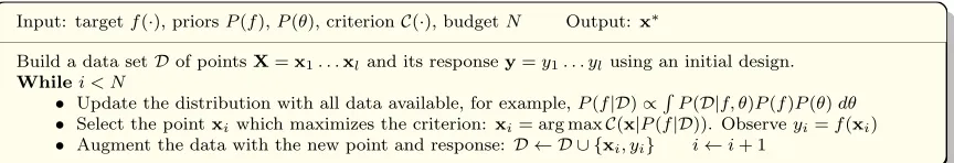
Input: targetf(·), priorsP(f),P(θ), criterionC(·), budgetN Output: x∗
Build a data setDof pointsX=x1. . .xland its responsey=y1. . . ylusing an initial design. Whilei < N
• Update the distribution with all data available, for example,P(f|D)∝R
P(D|f, θ)P(f)P(θ)dθ
• Select the pointxiwhich maximizes the criterion: xi= arg maxC(x|P(f|D)). Observeyi=f(xi) • Augment the data with the new point and response: D ← D ∪ {xi, yi} i←i+ 1
Figure 1: General algorithm for Bayesian optimization.
process with nonzero mean function or as a semiparametric model. The library allows to define priors on w, σs2 and θ. The marginal posterior P(f|D) can be computed in closed form, except for the kernel parametersθ. BayesOpt allows to use different approximations based on empirical Bayes (Santner et al., 2003) or MCMC (Snoek et al., 2012) onP(θ|D).
2.1 Implementation
Efficiency has been one of the main objectives during development. We found evidence that updating θ every iteration might be unnecessary or even counterproductive (Bull, 2011). For empirical Bayes (ML or MAP of θ), we found that a combination of global and local derivative-free methods such as DIRECT (Jones et al., 1993) and BOBYQA (Powell, 2009) marginally outperforms gradient-based method, in CPU time, for optimizing θby avoiding the overhead of computing the marginal likelihood derivative.
One of the most critical components, in terms of computational cost, is the computa-tion of the inverse of the kernel matrixK−1(Rasmussen and Nickisch, 2010). We compared different numerical solutions and we found that theCholesky decomposition method outper-forms any other method in terms of performance and numerical stability. Furthermore, we can exploit the structure of the Bayesian optimization algorithm in two ways. First, points arrive sequentially. Thus, we can do incremental computations of matrices and vectors, except when the distribution of the kernel parameters P(θ|D) is updated. For example, at each iteration, we know that only nnew elements will appear in the correlation matrix K, that is, the correlation of the new point with each of the existing points. The rest of the matrix remains invariant. Thus, instead of computing the wholeCholesky decomposition of
K, beingO(n3), we just add a new row of elements to theCholesky decomposition, which is
O(n2). Second, finding the optimal decision at each iterationxi requiresmultiple queries of
the acquisition function from the same posterior C(x|P(f|D)) (see Figure 1). Thus, we can precompute some terms of the posterior and criterion functions that are independent of the query pointx. To our knowledge, this is the first software for Gaussian processes/Bayesian optimization that exploits the idea of precomputing terms for multiple queries.
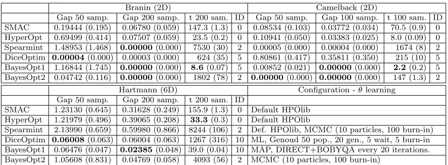
contin-Branin (2D) Camelback (2D)
Gap 50 samp. Gap 200 samp. t 200 sam. ID Gap 50 samp. Gap 100 samp. t 100 sam. ID SMAC 0.19444 (0.195) 0.06780 (0.059) 147.3 (1.3) 0 0.08534 (0.103) 0.03772 (0.034) 70.5 (0.9) 0 HyperOpt 0.69499 (0.414) 0.07507 (0.059) 23.5 (0.2) 0 0.10941 (0.050) 0.03383 (0.025) 8.0 (0.09) 0 Spearmint 1.48953 (1.468) 0.00000(0.000) 7530 (30) 2 0.00005 (0.000) 0.00004 (0.000) 1674 (8) 2 DiceOptim 0.00004(0.000) 0.00003 (0.000) 624 (35) 5 0.80861 (0.417) 0.35811 (0.350) 215 (10) 5 BayesOpt1 1.16844 (1.745) 0.00000(0.000) 8.6(0.07) 5 0.00852 (0.021) 0.00000(0.000) 2.2(0.2) 5 BayesOpt2 0.04742 (0.116) 0.00000(0.000) 1802 (78) 2 0.00000(0.000) 0.00000(0.000) 147 (1.3) 2
Hartmann (6D) Configuration -θlearning Gap 50 samp. Gap 200 samp. t 200 sam. ID
SMAC 1.23130 (0.645) 0.31628 (0.249) 155.9 (1.3) 0 Default HPOlib HyperOpt 1.21979 (0.496) 0.39065 (0.208) 33.3(0.3) 0 Default HPOlib
Spearmint 2.13990 (0.659) 0.59980 (0.866) 8244 (106) 2 Def. HPOlib, MCMC (10 particles, 100 burn-in) DiceOptim 0.06008(0.063) 0.06004 (0.063) 1267 (316) 10 ML, Genoud 50 pop., 20 gen., 5 wait, 5 burn-in BayesOpt1 0.06476 (0.047) 0.02385(0.048) 39.0 (0.04) 10 MAP, DIRECT+BOBYQA every 20 iterations. BayesOpt2 1.05608 (0.831) 0.04769 (0.058) 4093 (56) 2 MCMC (10 particles, 100 burn-in)
Table 1: Mean (and standard deviation) of the optimization gap, f(xbest)−f(xopt), and
time (in seconds) for 10 runs for different number of samples (including initial design) to illustrate the convergence of each method. ID represent the number of samples of the initial design for each algorithm and problem.
uous, discrete and categorical optimization. We also provide a method for optimization in high-dimensional spaces (Wang et al., 2013). The initial set of points (initial design, see Figure 1) can be selected using well-known methods such as latin hypercube sampling or Sobol sequences. BayesOpt relies on a factory-like design for the components of the opti-mization process. They can be selected and combined at runtime while maintaining a simple structure. This has two major advantages. First, it simplifies creating new components. For example, a new kernel can be defined by inheriting the abstract kernel or one of the existing kernels. Then, the new kernel is automatically integrated in the library. Second, inspired by the GPML toolbox by Rasmussen and Nickisch (2010), we can easily combine different components, like a linear combination of kernels or multiple criteria. This can be used to optimize a function considering an additional cost for each sample, for example, the cost of moving a sensor while maximizing the information (Marchant and Ramos, 2012). BayesOpt also implementsmetacriteria algorithms, like the bandit algorithm GP-Hedge by Hoffman et al. (2011) that can be used to automatically select the most suitable criteria during the optimization. Examples of these combinations can be found in Section 2.3.2.
The third objective is correctness. For example, the library is thread and exception safe, allowing parallelized calls. Parts that are sensible to numerical issues, such as the GP-Hedge algorithm, have been implemented with variation of the actual algorithm to avoid over- or underflow issues. The library internally uses NLOPT by Johnson (2014) for the inner optimization loops (optimize criteria, learn kernel parameters, etc.).
The library can be found at: https://bitbucket.org/rmcantin/bayesopt/
2.2 Compatibility
different compilers (Visual Studio, GCC, Clang, MinGW). The core of the library is written in C++, however, it provides interfaces for C, Python and Matlab/Octave.
2.3 Using the Library
There is a common API implemented for several languages and programming paradigms. Before running the optimization we need to follow two simple steps:
2.3.1 Target Function Definition
Defining the function that we want to optimize can be achieved in two ways. We can directly send the function (or a pointer) to the optimizer based on afunction template. For example, in C/C++:
double m y f u n c t i o n (unsigned i n t n q u e r y , const double ∗query ,
double ∗g r a d i e n t , void ∗f u n c d a t a ) ;
The gradient has been included for future compatibility. Python, Matlab and Octave inter-faces define a similar template function.
For a more object-oriented approach, we can inherit the abstract module and define the virtual methods. Using this approach, we can also include nonlinear constraints in the
checkReachability method. This is available for C++ and Python. For example, in C++:
c l a s s MyOptimization : public b a y e s o p t : : ContinuousModel {
public:
MyOptimization ( s i z e t dim , b o p t p a r a m s param ) : C o n t i n o u s M o d e l ( dim , param ) {}
double e v a l u a t e S a m p l e (const b o o s t : : n u m e r i c : : u b l a s : : v e c t o r<double>&q u e r y ) { // My f u n c t i o n h e r e };
bool c h e c k R e a c h a b i l i t y (const b o o s t : : n u m e r i c : : u b l a s : : v e c t o r<double>&q u e r y ) { // My c o n s t r a i n t s h e r e };
};
2.3.2 BayesOpt Parameters
The parameters are defined in the bopt params struct or a dictionary in Python. The details of each parameter can be found in the included documentation. The user can define expressions to combine different functions (kernels, criteria, etc.). All the parameters have a default value, so it is not necessary to define all of them. For example, in Matlab:
p a r . s u r r n a m e = ’ s S t u d e n t T P r o c e s s N I G ’; % S u r r o g a t e model and h y p e r p r i o r s % We combine E x p e c t e d Improvement , Lower C o n f i d e n c e Bound and Thompson s a m p l i n g
p a r . c r i t n a m e = ’ c H e d g e ( cEI , cLCB , c T h o m p s o n S a m p l i n g ) ’;
p a r . k e r n e l n a m e = ’ k S u m ( k M a t e r n I S O 3 , k R Q I S O ) ’; % Sum o f k e r n e l s
p a r . k e r n e l h p m e a n = [ 1 , 1 ] ; p a r . k e r n e l h p s t d = [ 5 , 5 ] ; % H y p e r p r i o r on k e r n e l
p a r . l t y p e = ’ L _ M C M C ’; % Method f o r l e a r n i n g t h e k e r n e l p a r a m e t e r s
p a r . s c t y p e = ’ S C _ M A P ’; % S c o r e f u n c t i o n f o r l e a r n i n g t h e k e r n e l p a r a m e t e r s
p a r . n i t e r a t i o n s = 2 0 0 ; % Number o f i t e r a t i o n s <=> Budget
p a r . e p s i l o n = 0 . 1 ; % Add an e p s i l o n−g r e e d y s t e p f o r b e t t e r e x p l o r a t i o n
Acknowledgments
References
James Bergstra, Remi Bardenet, Yoshua Bengio, and Bal´azs K´egl. Algorithms for hyper-parameter optimization. In NIPS, pages 2546–2554, 2011.
Eric Brochu, Vlad M. Cora, and Nando de Freitas. A tutorial on Bayesian optimization of expensive cost functions, with application to active user modeling and hierarchical reinforcement learning. eprint arXiv:1012.2599, arXiv.org, December 2010.
Adam D. Bull. Convergence rates of efficient global optimization algorithms. Journal of Machine Learning Research, 12:2879–2904, 2011.
Katharina Eggensperger, Matthias Feurer, Frank Hutter, James Bergstra, Jasper Snoek, Holger Hoos, and Kevin Leyton-Brown. Towards an empirical foundation for assessing bayesian optimization of hyperparameters. InBayesOpt workshop (NIPS), 2013.
Matthew Hoffman, Eric Brochu, and Nando de Freitas. Portfolio allocation for Bayesian optimization. In UAI, 2011.
Frank Hutter, Holger H. Hoos, and Kevin Leyton-Brown. Sequential model-based optimiza-tion for general algorithm configuraoptimiza-tion. In LION-5, page 507523, 2011.
Steven G. Johnson. The NLopt nonlinear-optimization package. http://ab-initio.mit.
edu/nlopt, 2014.
Donald R. Jones, Cary D. Perttunen, and Bruce E. Stuckman. Lipschitzian optimization without the Lipschitz constant. Journal of Optimization Theory and Applications, 79(1): 157–181, October 1993.
Roman Marchant and Fabio Ramos. Bayesian optimisation for intelligent environmental monitoring. In IEEE/RSJ IROS, pages 2242–2249, 2012.
Jonas Mockus. Bayesian Approach to Global Optimization, volume 37 ofMathematics and Its Applications. Kluwer Academic Publishers, 1989.
Michael J. D. Powell. The BOBYQA algorithm for bound constrained optimization with-out derivatives. Technical Report NA2009/06, Department of Applied Mathematics and Theoretical Physics, Cambridge England, 2009.
Carl E. Rasmussen and Hannes Nickisch. Gaussian processes for machine learning (GPML) toolbox. Journal of Machine Learning Research, 11:3011–3015, 2010.
Olivier Roustant, David Ginsbourger, and Yves Deville. DiceKriging, DiceOptim: two R packages for the analysis of computer experiments by kriging-based metamodelling and optimization. Journal of Statistical Software, 51(1):1–55, 2012.
Thomas J. Santner, Brian J. Williams, and William I. Notz. The Design and Analysis of Computer Experiments. Springer-Verlag, 2003.
Jasper Snoek, Hugo Larochelle, and Ryan Adams. Practical Bayesian optimization of ma-chine learning algorithms. In NIPS, pages 2960–2968, 2012.