Solving Inverse Problem Through Optimization and Its Application to Analog/RF IC Design.

(1)

ABSTRACT

WANG, YI. Solving Inverse Problem Through Optimization and Its Application to Analog/RF IC Design . (Under the direction of Paul D. Franzon.)

An inverse problem, which can be interpreted as finding out the design parameters given a set of specific output performance in most engineering problems, has perplexed human beings for a long time. In this dissertation, we particularly emphasis on addressing the inverse problem in analog/RF design field aiming to deliver a feasible circuit design through heuristic algorithms and statistical machine learning optimization method. The specific two challenges that we will focus on in analog/RF design are (1) Circuit IP redesign reuse. (2) EM simulation acceleration.

In this dissertation, we demonstrate the feasibility and efficiency of our proposed elec-tronics design automation flow in solving analog/RF design inverse problems within dif-ferent scenarios. The fundamental idea for incorporating statistical machine learning techniques into the simulation based design methodology is to leverage the surrogate models’ capability of modelling with limited data and predictions with uncertainty factor considered, which is a fit for the expensive SPICE/EM simulation. We extend this idea to cus-tomized interconnect design optimization, which integrates the concept of multi-fidelity to reduce the full wave EM simulation cost in analog/RF simulation based optimization problems.

(2)

(3)

Solving Inverse Problem Through Optimization and Its Application to Analog/RF IC Design

by Yi Wang

A dissertation submitted to the Graduate Faculty of North Carolina State University

in partial fulfillment of the requirements for the Degree of

Doctor of Philosophy

Computer Engineering

Raleigh, North Carolina 2020

(4)

DEDICATION

To my parents, Jianping Wang and Ying Wang, who always back me up in this long but beautiful journey. To my aunt, Dr. Min Wang, who shares the life advice with me when I

(5)

BIOGRAPHY

Yi Wang was born in Hangzhou, China and completed his pre-college education there in 2008. Then he moved to Chengdu, China and spent four years to obtain his Bachelor of Science in Microelectronics from University of Electronics Science and Technology of China. In August 2012, Yi started his graduate career as a Master student at North Carolina State University with Professor Alex Q. Huang for the research in power management integrated circuit. In August 2014, he decided to further his education as a Ph.D. student with Professor Paul Franzon to explore Machine Learning methods for electronics design automation.

(6)

ACKNOWLEDGEMENTS

I would like to give my utmost gratitude to my advisor, Dr. Paul D. Franzon for providing me with various research opportunities to explore within the team. The unprecedented research freedom helps me find the direction where I could devote myself and forges my career path in the electronics design automation. He is more of a life mentor than an educator, not only guiding his students in their way to great academic achievements but also inspiring us with his philosophy of life.

I would also like to express my deepest thank to Dr. Brian Floyd, who led me into the analog world. I could still recall the memory of the first class in ECE 511 analog electronics, which was also the first lecture I attended in this country. I am very grateful to Dr. Rhett Davis, who shares a lot of suggestions through our weekly meetings and daily discussions. I would also like to sincerely thank Dr. Min Chi, who is an amazing professor and a role model to me.

My gratitude also goes to the following people: My group fellows, Weiyi Qi, Zhuo Yan, Jong Boem Park, Zhao Wang, Kirti Bhanushali, Theodros Nigussie, Wenxu Zhao and Bowen Li, whom I kept friendship with during the past five years, though most of them have left the university and are pursing their new life goals. My friends in Monteith Engineering Research Center, Weihu Wang, Yi-Shin Yeh, Vikas Chauhan, Xiao Xiang, Junyu Shen, Yuan Chang and Tiantong Ren, who have made special pieces of the beautiful memory of the past years. My mentor in Hewlett Packard Enterprise, Chris Cheng, who led me into the magic machine learning world. My supervisor in Analog Devices, Dr. David Smart and colleagues, Dr. Brian Swahn, Sherry Yu, without whom I could not have made through it. My mentor in Cadence Design Systems, Dr. David White, who guided me to the new chapter of my career life.

(7)

LIST OF TABLES

Table 2.1 Van der Corput Sequence . . . 14

Table 2.2 S1 and ST Sobol Analysis (80 sample ) . . . 25

Table 2.3 S2 Sobol Analysis (80 sample ) . . . 25

Table 2.4 S1 and ST Sobol Analysis (400 sample) . . . 25

Table 2.5 S2 Sobol Analysis (400 sample) . . . 26

Table 2.6 S1 and Delta DMIM Analysis (80 samples) . . . 27

Table 2.7 S1 and Delta DMIM Analysis (400 samples) . . . 27

Table 2.8 S1 and ST FAST Analysis (80 samples) . . . 29

Table 2.9 S1 and ST FAST Analysis (400 samples) . . . 29

Table 2.10 Morris Analysis (80 samples) . . . 31

Table 2.11 Morris Analysis (400 samples) . . . 31

Table 2.12 First Order Variance Analysis (80 samples) . . . 32

Table 2.13 First Order Variance Analysis (400 samples) . . . 33

Table 2.14 Mixer Design Summary . . . 34

Table 2.15 Sobol Result . . . 34

Table 2.16 DMIM Result . . . 35

Table 2.17 FAST Result . . . 35

Table 2.18 Morris Result . . . 35

Table 3.1 Mixer Design Summary . . . 48

Table 3.2 SVD result1 . . . 48

Table 3.3 PC explained variance . . . 49

Table 3.4 SVD result2 . . . 49

Table 3.5 VCO Design Summary . . . 50

Table 3.6 VCO Redesign Result . . . 51

Table 3.7 VCO Redesign with FoM 3.6 . . . 52

Table 3.8 Mixer Multi-Objective Optimization Result with PCA . . . 53

Table 3.9 Mixer Multi-Objective Optimization Result 2 with PCA . . . 54

Table 3.10 Mixer Multi-Objective Optimization Result 3 with PCA . . . 55

Table 3.11 Mixer Reuse Result . . . 55

Table 3.12 T-coil Design Summary . . . 57

Table 3.13 Optimization Process . . . 59

(10)

Table A.1 S1 and ST Sobol Analysis (Voltage Gain) . . . 105

Table A.2 S1 and ST Sobol Analysis(Noise Figure) . . . 107

Table A.3 S1 and ST Sobol Analysis(Lo_Feedthrough) . . . 109

Table A.4 S1 and ST Sobol Analysis(S11) . . . 111

Table A.5 S1 and ST Sobol Analysis(S22) . . . 113

Table A.6 S1 and delta DMIM Analysis(Voltage Gain) . . . 115

Table A.7 S1 and delta DMIM Analysis(Noise Figure) . . . 117

Table A.8 S1 and delta DMIM Analysis(Lo_RF_Feedthrough) . . . 119

Table A.9 S1 and delta DMIM Analysis(S11) . . . 121

Table A.10 S1 and delta DMIM Analysis(S22) . . . 123

Table A.11 S1 and ST FAST Analysis(Voltage Gain) . . . 125

Table A.12 S1 and ST FAST Analysis(Noise Figure) . . . 127

Table A.13 S1 and ST FAST Analysis(Lo_RF_Feedthrough) . . . 129

Table A.14 S1 and ST FAST Analysis(S11) . . . 131

Table A.15 S1 and ST FAST Analysis(S22) . . . 133

Table A.16 mustar and sigma Morris Analysis(Voltage Gain) . . . 135

Table A.17 mustar and sigma Morris Analysis(Noise Figure) . . . 137

Table A.18 mustar and sigma Morris Analysis(Lo_RF_Feedthrough) . . . 139

Table A.19 mustar and sigma Morris Analysis(S11) . . . 141

(11)

LIST OF FIGURES

Figure 2.1 Flow of SA . . . 13

Figure 2.2 example of unconditional and conditional distribution of Y[Bor07] 17 Figure 2.3 24 points Sobol Sequence . . . 24

Figure 2.4 24 points Random Sequence . . . 24

Figure 2.5 600 points Sobol Sequence . . . 24

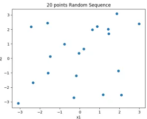
Figure 2.7 20 points DMIM Sequence . . . 26

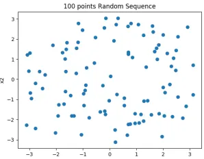
Figure 2.9 100 points DMIM Sequence . . . 26

Figure 2.11 70 points FAST Sequence . . . 28

Figure 2.13 100 points FAST Sequence . . . 28

Figure 2.15 30 points Morris Sequence . . . 30

Figure 2.17 60 points Morris Sequence . . . 30

Figure 2.19 Schematic of 79GHz Mixer . . . 33

Figure 3.1 Flowchart of Proposed Flow . . . 40

Figure 3.2 Flowchart of Surrogate Model . . . 42

Figure 3.3 Inductor . . . 46

Figure 3.4 Inductor Design Summary . . . 46

Figure 3.5 Inductance . . . 47

Figure 3.6 Paras. Cond. . . 47

Figure 3.7 SubstrateLoss . . . 47

Figure 3.8 Schematic of Mixer . . . 47

Figure 3.9 Schematic of VCO . . . 50

Figure 3.10 Tcoil Layout . . . 57

Figure 3.11 ADICE Optimization Result . . . 58

Figure 4.1 Overview of MFSBO-CS . . . 69

(12)

Figure A.3 S1& ST Lo_RF_Feedthrough . . . 110

Figure A.4 S1& ST S11 . . . 112

Figure A.5 S1& ST S22 . . . 114

Figure A.6 S1& delta Voltage Gain . . . 116

Figure A.7 S1& delta Noise Figure . . . 118

Figure A.8 S1& delta Lo_RF_Feedthrough . . . 120

Figure A.9 S1& delta S11 . . . 122

Figure A.10 S1& delta S22 . . . 124

Figure A.11 S1& ST Voltage Gain . . . 126

Figure A.12 S1& ST Noise Figure . . . 128

Figure A.13 S1& ST Lo_RF_Feedthrough . . . 130

Figure A.14 S1& ST S11 . . . 132

Figure A.15 S1& ST S22 . . . 134

Figure A.16 mu∗_&_σ_{Voltage Gain . . . 136}

Figure A.17 mu∗_&_σ_{Noise Figure . . . 138}

Figure A.18 mu∗&σLo_RF_Feedthrough . . . 140

Figure A.19 mu∗_&_σ_{S11 . . . 142}

(13)

CHAPTER

1 INTRODUCTION

1.1 Motivation

(14)

challenging nowadays due to its intrinsic complexity and NP-hardness. Consequently, the reuse of the design knowledge from the old technology, e.g., the circuit topology, device size, device type, supply voltage, etc., could accelerate porting IPs to the advanced node.

EM simulation acceleration.As the operating frequency goes up, the interactive electro-magnetic (EM) effect among components in high speed analog/RF circuit makes it harder for IC designers to achieve the optimal design parameters. Besides, as the passive structure becomes more cumbersome, the expensive EM simulation cost spent on verifying the designer’s attempts becomes critical in the whole design process[Sul13].

For the first two challenges mentioned above, inverse problem solving techniques based on SPICE simulation data are introduced. The conventional methodologies addressing the mathematical inverse problem can be summarized into numerical and statistical ap-proaches. Generally, the regularization based numerical methods usually require solvable models or analytical equations that can be easily transformed to a matrix format. Besides, the ill-posedness from the problem itself leads to unstable solution even if various regu-larization methods are researched and developed[Han90]. The statistic inversion theory seems to overcome the non-analytical ground truth of circuit system and ill-posedness by introducing random variables and their probability distribution to describe the unknown [Sil03]. However, let alone the proper use of prior, the extensive computation cost to realize the posterior distribution for high dimension applications would be another concern when applying such algorithms in real engineering problems.

(15)

At the design optimization phase, a sequentially sampling method is applied to determine the best design parameters based on the current surrogate model and then the surrogate is updated with the newly acquired data to achieve the better accuracy in the area where potential optimal lies. Within the proposed flow, both local design space near the optimal starting point and the entire design space would be explored by multiple groups of data during the design optimization phase to avoid the system stuck at a local optimal to a certain extent. Besides, the best sample from each group that have been verified with surrogate will be validated with the simulator and then be used to update the surrogate in a batch mode. This mechanism not only delivers additional coverage of design space but also helps increase the accuracy of the surrogate model efficiently by updating multiple samples within one iteration. This in return assists the proposed adaptive method to generate better samples for the optimization task. Moreover, the proposed flow should be capable to handle mixed integer problem, i.e., the design contains integer and continuous design variables where it could be a very common scenario in analog/RF design.

1.1.1 State of the Art

1.1.1.1 Forward Model

(16)

the rest focus on regularization techniques delivering the numerical solution. Regularization Method

We start with a simple example ofLaplace transformationand consider the following equation

L{f(s)}=

Z

e−s tf(t)d t (1.1)

where f (t)is a real function, then we approximate the integral with finite samples in s domain and apply the sum among the samples as shown below:

Z

e−sjt_{_f(_t)_}_{d t} _≈X_w

ke−sjtkf(tk) (1.2)

Let’s definexk = f(tk),yj =L{f(sj)}, andaj k =wke−sjtk and thus the format of Ax=y is written.wk andtk could be obtained from quadrature rule. Please note A is generally defined as the operator fromH1→H2, whereH1&H2are two separable Hilbert spaces.

The corrupted estimation result will be produced due to the large condition number of A,cond(A), i.e., the ratio of the largest to smallest singular value in singular value decompo-sition. Condition number indicates how many digits are lost in the calculation involved with A and a large condition number means ill-conditioned.

1. Truncated Singular Value Decomposition

In order to overcome the issues mentioned previously, regularization based methods were developed by trying to modify the original problem into one that is uniquely solvable and the error would not be of great difference between the approximate and exact answers. One classic method of them is called regularization by singular value truncation.

In[Han90], it gives out the theorem that: let A:H1→H2be a compact operator with

(17)

y, it leads to a unique solutionxk called truncated SVD solution which is

xk = k

X

n=1

1

λj

<y,un>vn (1.3)

In the finite-dimensional case, let A∈Rm×n and Ax=y, it is proved that the matrix A could be be singular value decomposed as:

A=UΛVT (1.4)

where U∈Rm×m and V∈Rn×n are orthogonal matrices.Λ∈Rm×n is a diagonal matrix whose items are called singular values. And equation 1.3 always has a solution in format of:

x =x0+A?y (1.5)

wherex0is one vector in kernel of A andA?is theMore-Penrose inverseof A. As a

matter of fact, the smallest singular values would be very closed to zero due to ill-posedness of A and thus lead to sensitivity of error in y. In practice the truncation index k in range of p is picked based ondiscrepancy principle, where 1≤p≤min(m,n).

2. Tikhonov Regularization

(18)

whereδis the regularization parameter. The choice of the valueδshould be made based on the noise level of the measurement y[Cal00].

Statistical Inversion Method

Another line of research work to solve inverse problem is to recast it as a problem of searching for the unknown from all existing information[Sak09]. The solution of such statistical inversion method would be the posterior probability distribution.

Regularization based methods tends to solve the inverse problem by modifying the problem itself to be solvable. Compared with regularization methods, statistical method produces estimation by the prior information that is often hidden and even doesn’t require a model of the formY =f(X,E).

One popular framework to address inverse problem statistically is from Bayesian infer-ence. The problem could be formulated as: Given the observation of Y, find the conditional probability distributionπ(x|yo b s e r v e d)of X. Then the posterior probability of distribution of X could be expressed as:

p(x|yo b s e r v e d) =

p(x)p(yo b s e r v e d|x) p(yo b s e r v e d)

(1.8)

The equation above is well known as Bayes’s formula and solving inverse problem could be divided into 3 sub-tasks:

• Find the right prior probability densityp(x)

• Find the likelihoodp(yo b s e r v e d|x)that describes the interaction between the obser-vation and the unknown

• Develop methods to derive posterior probability density

(19)

probability densityp(x|yo b s e r v e d)of the unknown X,xM AP follows:

xM AP =argmax p(x|yo b s e r v e d) (1.9)

Conditional Mean is also defined as:

xC M =E(x|y) =

Z

xπ(x|yo b s e r v e d)d x (1.10)

1. Posterior Distribution Exploration

As the solution to the inverse problem, single estimation of the posterior probabil-ity distribution could be found using maximum a posterior(MAP) or conditional mean(CM) and covariance. However, as the dimension of the parameter space in-creases, both methods would fail due to large computation cost needed. Markov Chain Monte Carlo method provide an alternative to determine samples from the posterior distribution that well approximate it.

In this section, we would first introduce the property oftime homogenous Markov chain:

µXj+1(Bj+1|x1, ....xj) =µXj+1(Bj+1|xj) =P(xj,Bj+1) (1.11)

where B are Borel sets and P is defined as theprobability transition kernel.

The first equality is well known as the probability of Xj+1depends on the present.

(20)

transition kernel P. P is invariant, aperiodic and irreducible. Then we could explore the given distribution by sampling it using such kernel mentioned above.

Metropolis Hastings algorithm[Has70]is one way to construct the transition kernel which satisfies thebalance equations. And proposed kernel is in the format of:

K(x,y) =α(x,y)q(y,x) (1.13)

whereq(x,y)is the called proposal distribution defining a transition kernel and the correction termαis shown as:

Q(x,A) =

Z

A

q(x,y)d y (1.14)

α(x,y) =min(1,π(y)q(y,x)

π(x)q(x,y)) (1.15)

The pseudo algorithm would be like:

• Pick initial valuex1and set k=1.

• Generate y fromq(xk,y)and calculate correction termα.

• Drawt ∈ [0, 1]from uniform probability density and if correction term α_≥ t, set xk+1=y, elsexk+1=xk. Stop until k=K.

Other algorithms that can be used to construct the transition kernel include Gibbs sampling[Gil], Slice sampling, Multiple try Metropolis[JSL], Reversible jump[Gre], etc.

1.2 Research Objective

(21)

re-• Analog/RF circuit block optimization.

• Analog/RF design inverse problem.

Why it is called the hybrid of regularization based and statistical Bayesian based method? In Tikhonov Regularization, it attempts to approach the x in an iterative way by minimizing the expression 1.6 and definitely it is a point estimation style method. It is suitable for the problem where A is difficult to identify in a analytic format. In Bayesian inverse theory, we have to use certain computation intensive methods to estimate posterior probability distribution of x. Instead of directly approximate posterior probability distribution of x, we inherit the idea of doing iterative optimization from regularization method through the single point posterior estimate of y.

The first two objectives above can be formulated into the same problem that seeks the specific design inputs under different circumstances.

From the perspective of optimization, there is no target value assigned to the flow and the flow will seek the best solution given a maximum number of function evaluation iterations.

(22)

three main components: design analysis; circuit redesign(optimization); circuit reuse. Due to the lack of successful analog layout synthesis tools, the majority of the optimiza-tion work menoptimiza-tioned beforehand stays at schematic level. In the chapter of 5, we outlook the challenges in the automation task to convert the schematic to layout, which will be our future research tasks.

1.3 Dissertation Organization

(23)

CHAPTER

2 ANALOG DESIGN ANALYSIS

(24)

2.1 Introduction

Sensitivity Analysis (SA) is the investigation of the variance of inputs and their impact on the outputs of the system we are interested. For practical engineering problems, sensitivity analysis becomes more important in design optimization and modelling due to great design complexity and high simulation cost to evaluate the design given the inputs values.

Generally,SAcould be categorized into two types, local and global sensitivity methodolo-gies. One typical implementation of localSAmethodology is one-at-time(OAT) approach. The local response of the outputs from the investigated system are obtained by varying one input factor at a time while keeping other inputs constant. The analysis is executed at some fixed point in the design space and thus it is called "local". The local type sensitivity analysis is limited to the incapability of capturing the interactions between input factors and the correct relation between inputs and outputs due to its nature of locality and assumption of linearity at evaluation point if the system is non-linear.

Today, global type sensitivity analysis methods are gaining more and more attention by overcoming the drawbacks of its local counterpart mentioned above. Generally, there are two schools within the globalSA, variance based and screening based methodologies. In the following sections, we will describe the theory behind the algorithms applied and discuss the simulation results from global sensitivity analysis

2.2 Global Sensitivity Analysis Methods

(25)

Figure 2.1Flow of SA

The major task of the first step is to generate a low discrepancy sample sequence with low computation cost, that is finding the specific sample sequences generated based upon different analysis methods. And in this study, we will review variance based Sobol, Delta Moment Independent Measure(DMIM), Fourier Amplitude Sensitivity Analysis(FAST) and screening based Morris and its improved version by Campolongo.

2.2.1 Variance based Methodologies

2.2.1.1 Sobol

(26)

First we would introduce the concept ofRadical Inversion. This calculation could be expressed as:

i = M−1

X

l=0

al(i)bl (2.1)

φb,C = (b−1, ...b−M)[C(a0(i), ...aM−1(i))]T (2.2)

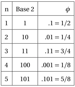
The two math equations above are used to describe the steps to generate Radical Inversion sequence: For the first step (equation 2.1), it transformsito be abbased number, and the most common selection is the binary decomposition. In the equation 2.2, the coefficient vectorai is multiplied with a generator matrix C, then the product vector is mirrored to the number smaller than 1. When C is identity matrix, the sequence generated is also called Van der Corput. The table below shows the example of Van der Corput sequence.

To be more detailed, if we want to convert 5 to Van der Corput sequence based number, 5 is first converted to 101 in binary setting, then mirrored to .101, which is .625. Here identity matrix C is used.

Table 2.1Van der Corput Sequence

n Base 2 φ

1 1 .1=1/2

2 10 .01=1/4 3 11 .11=3/4 4 100 .001=1/8 5 101 .101=5/8

The Van der Corput sequence has following properties:

(27)

The sobol sequence generation can be interpreted as a base 2 radical inversion with various generator matrix C for each input dimension, i.e., for each dimension, it is a Van der Corput Sequence with a non-identity matrix C as used in equation 2.2.

Theory

First, let’s assume the system we want to analyze is modelled as y=f(x), where the n dimensional input is x= (x1, ...xn). And it is useful to consider the xi as the mutually independent random variable uniformly distributed in[0,1]. Sobol’s method uses the de-composition of the model output variance into summands of input parameters in different dimensions given the assumption of ANOVA-representation of the f(x) as shown below [Sob01]:

f(x) =f0+

X

i=1

fi(xi) +

X

i<j

fi j(xi,xj) +...+f12...n(x1,x2, ...xn) (2.3)

if

Z 1

0

fi1...is(xi1, ...xis)d xk=0 (2.4)

fork =i1, ...is and 1≤i1<...<is ≤n. So we could have:

f0=

Z

f(x)d x (2.5)

fi(xi) =

Z

f (x)Y k6=j

d xk−f0 (2.6)

fi j(xi,xj) =

Z

f(x)Y k6=i,j

(28)

define:

Di1...is =

Z

f_i2

1...isd xi1...d xi s (2.9) So we could have[Sal10]:

D= n

X

s=1

n

X

i1<...<is

Di1...is (2.10)

The global sensitivity indices could be expressed as:

Si1...is = Di1...is

D (2.11)

For example, the first order contribution from ith input parameter to the output could be expressed as:

Si= Di

D (2.12)

the second order contribution from the interaction of ith and jth parameters could be expressed as:

Si j = Di j

D (2.13)

The total effect of one parameter on the output is calculated as:

ST i =Si+Si j+...+S1...i...s (2.14)

(29)

2.2.1.2 Delta Moment Independent Measure

Sample Method

Latin Hypercube Sample[Pli13].

Theory

The idea of Moment Independent based method is: First obtain the unconditional density distribution of Y, i.e.,fY(y), with all design parameters free. Then fix ith input atxi∗ and generate the conditional density distribution of Y, i.e.,fY|Xi(y). An illustration offY(y) and fY|Xi(y)are shown in figure 2.2 from[Bor07].

Figure 2.2example of unconditional and conditional distribution of Y[Bor07]

(30)

where fXi(xi)is the marginal density ofxi. Here we define:

δi= 1

2EXi(s(Xi)) (2.17)

So theδi is called the moment independent sensitivity indicator forXi. Similarly, the delta ofXi andXj is shown as:

δi j = 1

2EXiXj(s(Xi,Xj)) (2.18) where

s(Xi,Xj) =

Z

|fY(y)−fY|Xi,Xj(y)|d y (2.19)

In summary, largerδi means more variance for the output of the model for the ith input factor.

2.2.1.3 Fourier Amplitude Sensitivity Analysis (FAST)

Sample Method

Curve search is one typical sampling method in Fourier Amplitude Sensitivity Analysis. We will describe it in next section where it will naturally be applied to eliminate the multi-dimension integral calculation by introducing a new variable s[Cuk73].

Theory

The idea of FAST is to perform the ANOVA₋like decomposition of the variance of y, the output of the system with the input x using multidimensional Fourier transformation of f [Sal99]. The basic concept of FAST is very close to Sobol’s sensitivity analysis method while it could be more computationally efficient.

Any f(x) in unit hypercube can be Fourier expanded as the following format[Wik]:

f (X1, ...,Xn) = ∞

X

m1=−∞ ...

∞

X

mn=−∞

Cm1...mne

(31)

The ANOVA₋like decomposition of f(x) could be expressed as:

f0=C00...0 (2.21)

fj =

X

mj6=0

C0...mj...0e

2πi(mjXj) _(2.22)

fj k=

X

mj6=0

X

mk6=0

C0...mj...mk...0e

2πi(mjXj+mkXk) _(2.23)

where the Fourier coefficient is in a format of:

Cm1...mn =

Z 1

0

...

Z 1

0

f(X1, ...,Xn)e2πi(m1X1+...mnXn)dX1...dXn (2.24)

The first order variance could be calculated by:

Vj =

Z 1

0

f_j2(Xj)d Xj =

X

mj6=0

|C0...mj...0|

2₌₂

∞

X

mj=1

A2_{m j}+B_{m j}2 (2.25)

whereAm j andBm j are the real and imaginary part of the fourier coefficientC0...mj...0which could be calculated with equation 2.24 as:

Am j =

Z 1

0

...

Z 1

0

f(X1, ...,Xn)c o s(2πmjXj)dX1...dXn (2.26)

Bm j =

Z 1

0

...

Z 1

0

f(X1, ...,Xn)s i n(2πmjXj)dX1...dXn (2.27)

(32)

As s varies, all the factors change simultaneously along a curve that explores design space. Eachxi oscillates periodically atwi. The oscillation of y at frequencywiwill have a high amplitude if the ith factor has strong impact on the output.

One widely used search curve is shown below

Xi= 1 2+

1

πarcsin(sin(wis+φi)) (2.28)

To make the exploring curve be able to arbitrarily close to any point in input domain, the wi should be chosen to be incommensurate to the order of M following

n

X

j=1

γjwj 6=0 for n

X

j=1

|γj| ≤M+1 (2.29)

Therefore, we could have

Am j = lim T→∞

1 2T

Z T

−T

f(X1(s)...Xn(s))c o s(2πmjXj(s))d s (2.30)

Bm j = lim T→∞

1 2T

Z T

−T

f(X1(s)...Xn(s))s i n(2πmjXj(s))d s (2.31)

Using positive integerwi, this one dimension integral is periodic and only the integration over 2πis required.

Am j ≈ 1 2π

Z π

−π

f(X1(s)...Xn(s))c o s(2πmjXj(s))d s (2.32)

Bm j ≈ 1 2π

Z π

−π

f(X1(s)...Xn(s))s i n(2πmjXj(s))d s (2.33)

(33)

2.2.2 Screening based Methodology

2.2.2.1 Morris Sensitivity Analysis

Basic Morris Sample Method

Morris sensitivity analysis is based on the research of elementary effects. So the concen-tration of this method would be focusing on how to generate the sample points.

The basic sample method of Morris screening method was proposed in[Mor91]. The assumption made in this work is that the ith input elementary effect could be approximated as a distributionFi, where the elementary effect of ith input parameter at jth sample with level l could be defined as:

d_ij = f (q j₊_∆_e

i)−f(qj)

∆ (2.34)

where

∆∈ { 1

l −1, 2

l −1, ..., 1− 1

l −1} (2.35)

For r samples,Fiis described as:

µ∗ i = 1 r r X

j=1

|d_ij(q)| (2.36)

σ2

i = 1 r−1

r

X

j=1

(d_ij(q)−µi)2 (2.37)

(34)

Morris sample generation:

Suppose k=2, l=4, we choose∆=2/3(One elementary effect in one sample), seed value= [1/3,1/3], therefore,

D∗=

 

1 0

0 −1

 P∗=

 

0 1 1 0

 B=

     0 0 1 0 1 1      J =      1 1 1 1 1 1      (2.39)

So the sample matrix would be:

B∗=

    

1 1/3

1 1

1/3 1

     (2.40)

This method only need to k+1 runs compared with 2rk runs if∆is randomly selected fromFi to yield elementary effects. One suchB∗is called one trajectory and if a sample of r effects is required fromFi, then r independentB∗could be concatenated to form the sample matrix.

After evaluate the samples using the model, we could obtain theµ∗_and_σ2_{. High}_µ∗ i

means ith input has more impact on output and highσ2

i illustrates ith input might have more interaction with other input parameters.

2.2.2.2 Campolongo enhanced Morris Sensitivity Analysis

Based on the original Morris screening method, Campolonge made several improvement that could summarized as follows[Cam07]:

(35)

Morris trajectories,_≈500₋1000. And then choose r trajectories with highest spread, i.e., the trajectories with r largest distance between each other.

• useµ∗_{where it is the estimation of the mean of the distribution of the absolute values} of the elementary effects.

• If the model has large amount of input factors, the usage ofµ∗_{could lead to grouping} of factors, i.e., to produce an overall sensitivity analysis for a group of factors.

2.3 Results and Analysis

In this section, we first demonstrate the 2 Dimensional sample points generated by the sample generation stage from various sensitivity analysis, intuitively showing the sequence quality determined by discrepancy. In the next part, we will illustrate the results from different sensitivity analysis for same 3D problem where the number of sample points are set to be equal.

The 3 input dimension test function used in this report isIshigami Function, which is expressed as:

f(x) =sin(x1) +asin(x2)2+bx₃4s i n(x1) (2.41)

(36)

Figure 2.324 points Sobol Sequence Figure 2.424 points Random Sequence

Figure 2.5600 points Sobol Sequence Figure 2.6600 points Random Sequence

2.3.1.2 Sensitivity Analysis

(37)

Table 2.2S1 and ST Sobol Analysis (80 sample )

Parameter S1 S1_conf ST ST_conf

x1 -0.2034 0.6427 1.3458 2.0318

x2 0.8383 0.6078 0.7169 0.5375

x3 -0.5920 0.3756 0.4598 0.3601

Table 2.3S2 Sobol Analysis (80 sample )

Parameter1 Parameter2 S2 S2_conf

x1 x2 0.2086 1.1477

x1 x3 1.1652 0.9111

x2 x3 0.2685 0.7940

400 samples result as below:

Table 2.4S1 and ST Sobol Analysis (400 sample)

Parameter S1 S1_conf ST ST_conf

x1 0.3159 0.2877 0.7038 0.5235

x2 0.4693 0.3012 0.5091 0.1938

(38)

Table 2.5S2 Sobol Analysis (400 sample)

Parameter1 Parameter2 S2 S2_conf

x1 x2 0.1130 0.4325

x1 x3 0.7040 0.7869

x2 x3 0.2615 0.3002

2.3.2 Delta Moment Independent Measure

2.3.2.1 Sample Sequence

(39)

80 samples DMIM analysis result. In Table 2.6, delta means the total moment independent sensitivity indice value of each variable and delta_conf is the standard deviation of delta given 0.95 confidence level. A smaller delta_conf means delta observed is more likely to be accumulated near the value we obtained. S1 is defined as the first order moment independent sensitivity indice value of each variable.

Table 2.6S1 and Delta DMIM Analysis (80 samples)

Parameter delta delta_conf S1 S1_conf

x1 0.1584 0.0838 0.1750 0.1454

x2 0.0882 0.0591 0.1417 0.0940

x3 0.1002 0.0580 0.0277 0.0847

Table 2.7S1 and Delta DMIM Analysis (400 samples)

Parameter delta delta_conf S1 S1_conf

x1 0.1227 0.0317 0.2087 0.0648

x2 0.1924 0.0427 0.1960 0.0650

(40)

2.3.3 Fourier Amplitude Sensitivity Analysis

In order to numerically calculateAm j which is a one dimension integral, we would use 2q+1 sample points to approximate the integral. The number of sample points should satisfy Nyquist criteria which is related to interference parameter M andwm a x, the largest frequency in set of incommensurate frequency. In this implementation, sample number N should be larger than 4M2₌_64.

Figure 2.1170 points FAST Sequence Figure 2.1270 points Random Sequence

(41)

80 sample FAST result

Table 2.8S1 and ST FAST Analysis (80 samples)

Parameter S1 ST

x1 0.3094 0.5523

x2 0.6688 0.6936

x3 0.0054 0.2532

Table 2.9S1 and ST FAST Analysis (400 samples)

Parameter S1 ST

x1 0.3072 0.5525

x2 0.4442 0.4888

(42)

2.3.4 Morris Sensitivity Analysis

Figure 2.1530 points Morris Sequence Figure 2.1630 points Random Sequence

Figure 2.1760 points Morris Sequence Figure 2.1860 points Random Sequence

(43)

Table 2.10Morris Analysis (80 samples)

Parameter µ∗ µ µ∗_conf σ

x1 7.079 7.079 2.668 6.379

x2 7.875 -0.788 0 8.039

x3 4.374 0.625 2.668 7.559

Table 2.11Morris Analysis (400 samples)

Parameter µ∗ _µ _µ∗_{_conf} _σ

x1 6.964 6.954 1.187 6.235

x2 7.875 0.630 0 7.889

x3 7.374 0.875 1.129 9.608

2.3.5 Comparison of different sensitivity analysis

(44)

Table 2.12First Order Variance Analysis (80 samples)

Parameter Morrisµ∗ Sobol S1 DMIM delta FAST S1

x1 7.079 -0.2034 0.1584 0.3094

x2 7.875 0.8383 0.0882 0.6688

x3 4.374 -0.5920 0.1002 0.0054

From table 2.12, the sensitivity analysis results from Morris, Sobol’s and FAST are con-sistent where x2 influence most, followed by x1, x3.

DMIM delivers different solution, which could be explained by the factor that a parame-ter influencing output variance most may not change the output distribution most. DMIM only considers the influence of one input varible to the output variance while the other three calculate the output distribution in the sample analysis stage. When taking the entire output distribution into consideration, x1 is the most important followed by x3 and x2.

Next, we start to look at the second order variance that involves the interaction of two input factors. From Table 2.2, it is clear to find the total indice of x1 is significantly larger than S1 and similar result applies to x3. That means second or higher interaction variances plays important role in x1 and x3 so far. And this is proved by Table 2.3 where it shows S2 of x1 and x3 is much larger than S2 of x1 and x2, x2 and x3, respectively. This result is also confirmed with Table 2.4 that ST of x1 and ST of x3 are significantly larger that their S1 while S1 and ST of x2 are close in value. The Morris screening analysis seems to provide the opposite result that the influence of x2 is prone to be dependent on other inputs followed by x3, x1 from theσvalue in Table 2.10. One possible explanation would be that only 20 trajectories are used in Morris sampling stage and probably more trajectories are needed to get better coverage of design space.

(45)

Table 2.13First Order Variance Analysis (400 samples)

Parameter Morrisµ∗ Sobol S1 DMIM delta FAST S1

x1 6.954 0.3159 0.1227 0.3072

x2 7.875 0.4693 0.1924 0.4442

x3 7.374 0-0.2483 0.1241 0.0001

From table 2.13, the sensitivity analysis results from Morris and DMIM are consistent where x2 influence most, followed by x3, x1, while Sobol and FAST still follows the same importance sequence in 80 samples sensitivity analysis. It could be explained that FAST and SOBOL’s only use the output decomposition to quantify the input factors sensitivity by using variance while DMIM and Morris are to identify which input variables are contributing significantly to the output uncertainty using both inputs and outputs.

2.3.6 Sensitivity Analysis on RF circuit

(46)

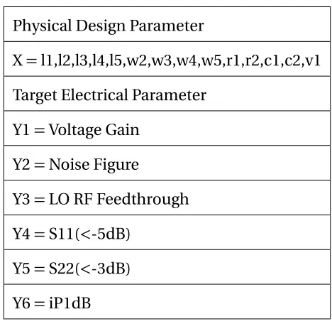
Table 2.14Mixer Design Summary

Physical Design Parameter

X=l1,l2,l3,l4,l5,w2,w3,w4,w5,r1,r2,c1,c2,v1 Target Electrical Parameter

Y1=Voltage Gain Y2=Noise Figure

Y3=LO RF Feedthrough Y4=S11(<-5dB)

Y5=S22(<-3dB)

2.3.6.1 Analysis Summary

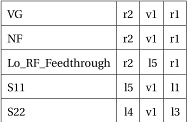
The detailed analysis data is documented in Appendix A. Here we summarize the results from the observation of the four sensitivity analysis methods. We discover that the SA results from Sobol and FAST are consistent and they could be used as the tools to unveil the relation between design variables and outputs. For simplicity of showing results in following tables, VG is used to stand for voltage gain, NF for noise figure. The 3 design variables whose first order sensitivity indice ranking in top 3 from our analysis are selected as illustrated from Tables 2.15 to 2.18.

Table 2.15Sobol Result

VG r2 v1 r1

NF r2 v1 r1

Lo_RF_Feedthrough r2 l5 r1

S11 l5 v1 l1

(47)

Table 2.16DMIM Result

VG w2 c2 r1

NF l5 l1 r1

Lo_RF_Feedthrough l1 l5 l2

S11 r2 w2 r1

S22 w2 c1 w4

Table 2.17FAST Result

VG r2 v1 r1

NF r2 v1 r1

Lo_RF_Feedthrough c2 l5 v1

S11 l5 v2 l1

S22 c2 l4 v1

Table 2.18Morris Result

VG v1 r1 l3

NF l2 v1 r1

(48)

follows.

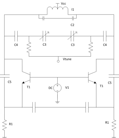
• Voltage GainGenerally the voltage gain of the example mixer circuit is related to the transconductance of transistors and load at the output port. The possible design variables related to transconductance in the example mixer are v1, l1. r1 and r2 are the design features that bond to the load of the output where r1 could also be served to control bias current of the circuit.

• Noise FigureNormally the noise figure is associated with the optimal current density of the transistors in the RF circuit. Since this performance is current related, v1, r1 and r2 are both critical to achieve better noise figure. Input matching plays an important role in noise figure as well. Thus, l2 could be a potential design variable that should be considered for eliminating noise figure.

• Lo RF FeedthroughBasically, this performance is coupled with the signal path from RF input port to local oscillator input port. l5, v1, l1, l2 and c2 are possible variables that contribute most to lo rf feedthrough.

• S11S11 in this design case is related to local oscillator input port. So l5, v1, and l1 should be well designed if S11 is the key specification in your work.

• S22S22 in this design case has related to the RF input and transistors. Therefore, l4, l3, v1, l1 are the design variables considered important for S22.

(49)

describe the authentic output, which leads to the inappropriate expectation calculation of the input variance to the output.

(50)

CHAPTER

3 RFIC IP REDESIGN AND REUSE

(51)

3.1 Introduction

This work addresses the problems of circuit block migration between different technology nodes, and circuit optimization within one node for different goals. i.e., given a transistor netlist, how do we redesign a circuit quickly and optimally? At its core, this is a transistor and passive sizing problem.

As the demand for short time to market (TTM) of IC products increases, analog/RF IC designs becomes more and more challenging. In the late 1980s, the first knowledge based analog synthesis tools appeared to encode design expertise in fixed computer executable form to acquire desired design[Deg87]. Later, OASYS , MIDAS[Bee93]and other tools have been developed but the disadvantage of knowledge based methods that comes from its inflexibility for various designs and time needed for redefining plans for new topologies and performance targets still existed. On the other hand,optimization based method applying mathematical optimization techniques to solve analog sizing became popular. It turns the complex analog design into a task which is to find the optimal values in the input design space via different optimization algorithms. The advantage of optimization based method is that the flow could be reused for various scenarios and its accuracy mostly depends on the accuracy of the semiconductor device model. In the past decades, the usage of optimization based methods was subject to computation capability due to its nature of huge amount of object function evaluations involved to obtain results.

(52)

3.2 Analog IP Redeign & Reuse Flow

3.2.1 Overview of Proposed Design Flow

We propose a computationally effective methodology flow for analog/RF design aiming to implement analog synthesis for fixed topology. It includes design analysis, optimization and reuse as shown in Fig. 3.1.

Figure 3.1Flowchart of Proposed Flow

3.2.2 Design Space Analysis

(53)

For a p-by-n matrix M, there exists a diagonal p-by-n matrix with non-negative real number in the form of equation 3.1 as follows:

X =UΣVT (3.1)

XTX =VΣ2VT (3.2)

The diagonal entries ofΣare called singular values of M. The interpretation of SVD is that it decomposes the small size dataset generated for design analysis in a set of orthogonal components after rotation/scaling and the diagonal matrix together with U, V presents the amount of the variance in the selected principle components. In this work, we develop a fully automated parser to process design analysis and applied to 79G mixer case. The components are selected based on the algorithm as follows: 1) Run singular value decom-position analysis; 2) Obtain the first largest 6 principle components(PC), and then select the circuit components with largest 2 absolute value of explained variance in each PC; 3) Remove the duplicated components in step (2); 4) Output result for further design space modification.

3.2.3 Surrogate Modeling Method

(54)

more samples in the region where either there might exist optimal solution or it is not explored. 4) Model is evaluated and validated. The Fig. 3.2 below shows more detailed steps in surrogate modeling.

In this work, model builder is set to mixture of Kriging with Gaussian correlation function and cubic radial basis function. The adaptive sample methods will be discussed in next section below.

Figure 3.2Flowchart of Surrogate Model

3.2.4 Adaptive Sample Strategy

In surrogate modeling, one-shot samples from the initial sampling plan are usually not enough to construct the globally feasible model due to many unknown non-linearity and discontinuity in the target mapping function. Adaptive sampling strategy allows to search for new samples whose locations are not explored yet by analyzing current response surface.

(55)

method and candidate point search as the final solution.

Expected Improvement: Expected Improvement[Jon98]is a typical acquisition func-tion in the field of Bayesian optimizafunc-tion. From the view of surrogate modeling, Bayesian optimization is a special case where the model builders are statistical based methods as Gaussian Process, Student-t, etc. and adaptive sample methods are probability of improve-ment, expected improveimprove-ment, etc. Bayesian optimization works by constructing a posterior distribution of functions that describes a Gaussian process. As the number of observations grows, the posterior distribution improves and it becomes more certain of the regions in design space to be explored. Equation 3.3 shows the mathematic expression of expected improvement[Jon98]and the algorithm tends to maximizeα_{E I} by

αE I(x;θ,D) =σ(x;θ,D)(y(x)Φ(y(x))) +N(y((x); 0, 1)) (3.3)

wherey(x) = f(xb e s t)−µ(x;θ,D)

σ(x;θ,D) . Clearly, expected improvement would be prone to search those areas that with either best function value or largest uncertaintyσin order to maximize equation 3.3. However, as the dimension of design parameters increases, the computation cost for maximizing equation 3.3 becomes critical in practical engineering. In VCO case, we first applied Bayesian optimization after transforming integer constraints to continuous conditions. For comparison, we then implement candidate point search (CAND) to illustrate the advantage of CAND in optimizing such problem.

(56)

algorithm require a large number of function evaluations to find global optimum.

Thus, a new sample strategy, candidate point search is applied in Analog/RF circuit design for the first time hoping to solve drawbacks of existing methods. Candidate point search method not only solves the concerns mentioned above, but also could be used in large dimensional design space without the issue of computation cost raised in Bayesian optimization. It is adapted and improved from[MüL13], and the steps of candidate point search algorithm is given below: Step 1: Find variables to perturb 1)Evaluate objective function at initial points, and update counter; 2)Group1: perturbation only continuous variables of best point by random select from D variables for inclusion through probability calculationP =10/data_{d i m}when data dimension>10 and 1 when data dimension<10; Random select perturbing rate. Group2: Perturbation only discrete variables of best point. Group3: Perturbation continuous and discrete variables of best point. Group4: Random sample in design space. Then compute function value based on existing response surface for 4 groups. Step 2: Compute scoring criteria Determine distance of each candidate point to the set of already sampled and do min-max normalization and discard points that are close to sampled points. Step 3: Find best candidate & perform func. evaluation Normalize predicted function values and generate candidate total value for weighted sum of scaled distance and scaled function values. Step 4: Find index of best candidate and perform expensive function evaluation at selected point. Go to Step 1 until criterion is met.

(57)

3.2.5 Nu-SVM

On-chip inductors are key components in RFIC - used for filtering and tuning. Recently, some foundries started to offer inductor models which suffers inaccuracy issue in generating SPICE parameters in netlist. In some multi-GHz RF front end designs, designers have to implement their own spiral inductors in the range of sub-nH where the standard inductor cell from foundries don’t support. RF designers have to manually redesign the size of inductor in EM simulator and extract it to SPICE if the circuit performance don’t meet their requirements. However, this trivial but essential work requires time and usually would delay TTM to some extent.

We proposed to use machine learning techniques to do circuit-inductor co-optimization. In this work, we applied Nu-SVM regressor as the model method and integrated the model into surrogate based optimization design flow so the tedious inductor redesign could be done automatically.

The idea behind SVM is to find a set of hyper-planes that maximize the geometric margins between training dataset and planes. For SVM regression, training a hyper-plane can be expressed in equation 3.4,

minimize1 2|w|

2

s.t._|yi−<w,xi>−b| ≤ε (3.4)

(58)

3.3 Experiment Result

3.3.1 Nu-SVM Inductor Model

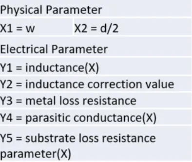
In this work, an octagonal spiral on-chip inductor as shown in Fig. 3.3 was modeled based on limited EM simulation result points for VCO design. Fig. 3.4 summarizes the design input parameters and desired outputs. The coefficientR2_{is used to evaluate the model}

Figure 3.3Inductor

Figure 3.4Inductor Design Summary

quality. The figures 3.5 to 3.7 below show the actual vs. predicted inductance, parasitic conductance and substrate loss resistance for the test dataset, respectively. The orange dots are actual results, blue dots are predicted results.

The model score is calculated as the uniform weighted sum of coefficientR2_{from 3}

(59)

Figure 3.5Inductance Figure 3.6Paras. Cond. Figure 3.7SubstrateLoss

3.3.2 Design Analysis

(60)

Table 3.1Mixer Design Summary

Physical Design Parameter

X=l1,l2,l3,l4,l5,w2,w3,w4,w5,r1,r2,c1,c2,v1 Target Electrical Parameter

Y1=Voltage Gain Y2=Noise Figure

Y3=LO RF Feedthrough Y4=S11(<-5dB)

Y5=S22(<-3dB) Y6=iP1dB

From design perspective, the importance of each performance is ranked as: VG>iP1dB

>S11>S22>Lo_RF_Feedthrough>NF. That is to say, designers should focus on VG optimization more than iP1db, etc,. This general scheme is working for the scenario that the first few PCs contribute similar variance in the newly transformed space, especially for a high dimensional space.

Table 3.2SVD result1

VG NF LO RF Feedth. S11 S22 iP1dB

PC1 _Ø _Ø

PC2 Ø Ø

PC3 Ø Ø

PC4 _Ø _Ø

PC5 Ø Ø

(61)

In the mixer design case (6 input dimension), we also discover that the normalized variance for each principal component is as follows in Table 3.3 :

Table 3.3PC explained variance

PC1 PC2 PC3 PC4 PC5 PC6

0.4920 0.2209 0.1572 0.074 0.048 0.006

Since PC1 contributes nearly 50% of the total variance in the dataset. Another strategy to select the most important features is sorting the first principal component and rank the features according to the variance in one PC. The resulting importance is VG>iP1dB>NF

>S22>S11>Lo_RF_Feedthrough.

Table 3.4SVD result2

VG NF LO RF Feedth. S11 S22 iP1dB

PC1 -0.5741 0.5625 0.018 -0.095 0.1459 -0.5684

3.3.3 IP Redesign & Reuse

3.3.3.1 IP Redesign

(62)

Figure 3.9Schematic of VCO

Table 3.5VCO Design Summary

Physical Design Parameter X=l1,C1,C2,C3,C4,C5,T1,R1 Target Electrical Parameter Y1=Phase Noise @ 1MHz offset

(63)

Table 3.6VCO Redesign Result

PN @ 1M offset Center Freq

CAND Mixed Integer Opt. -123.45 9.605G

CAND Mixed Integer Opt. (Single Objective) -123.1 9.546G

CAND Continuous Opt. -122.91 10.3G

Bayesian Opt -118.8 9.95G

Manual Design -122.2 10G

For 1st and 2nd experiment shown in the Table 3.6, we are trying to explore to establish figure of merit (FoM) for VCO in our case. Since the 2nd performance goal is set to be a range of center frequency, we first simply set FoM to be 3.5:

FoM=_L(∆f)−20log(fo/1010) (3.5)

(64)

in equation 3.6[Kin99]:

FoM=_L(∆f) +10log( PD C

1mW) +20log(

∆f f0

) (3.6)

The first term of equation 3.6 is the phase noise measured at an offset frequency∆f. In this case, 1MHz is chose for the calculation in Table 3.7. The second term is the normalized DC powerPD Csince the it is measured in mW. The third term explained in equation 3.6 is related to the center frequency of the design. A VCO design with a higher center frequency tends to have a better FoM but the other two terms could be worse. Generally a well designed VCO should generate less phase noise and consume less power. By executing the flow on the FoM, we obtain the result in Table 3.7.

Table 3.7VCO Redesign with FoM 3.6

PN @ 1MHz Center Freq Tuning Range Power FoM(3.6)

Our method -120.90 9.6G 6.99% 0.051W -182.1

Human Design -122 10G 13.7% N/A -187

Case 2 Mixer For mixer design case, we first demonstrate the feasibility of applying PCA to weight setting in multi-objective analog design problem. The idea behind this methodology is that we hope to set up proper initial multi-objective weights through PCA analysis. Then minor modifications on weights are made to meet the performance requirements through multi-objective optimization.

(65)

function value of 50 is given if S11 is larger than -5 and S22 is larger than -3.

objective function=-VG+NF+LO/50 - iP1db (3.7)

The resulting optimal result is displayed in Table 3.8.

Table 3.8Mixer Multi-Objective Optimization Result with PCA

8HP 8XP Manual Design

Voltage Gain 7.201 18.28

Noise Figure 12.019 9.39

LO RF Feedthrough -51.440 -27.59

S11 -9.166 -4.6 (not met)

S22 -6.792 -3.3

iP1dB 2.242 -4.67

The optimized design variables are 99.38u, 14.243u, 285.98u, 14.243u, 1.368, 99.99, 908.24, 2.405p, 47.842u, 5.552u, 107.8u, 8.112u, 22.336f, 5.297u.

After 1st round optimization, we found out that noise figure was worse than manual design. Thus we increased the weight of noise figure as indicated in the second objective function 3.8:

(66)

Table 3.9Mixer Multi-Objective Optimization Result 2 with PCA

S11 -6.3 -4.6 (not met)

S22 -11 -3.3

iP1dB -9.79 -4.67

The most challenging part in this mixer design is to set a proper weight for iP1dB. iP1db could be either as good as a positive number or a negative, which leads to the vagueness in weight sign setting. After 2nd round optimization, we found iP1db got worse so we reduced the weight of it assuming negative iP1dB. Meanwhile, we found Lo RF feed through had room for performance trade-off so we lowered its weight a little bit. In the third round of optimization, a new objective function of 3.9 is formulated:

objective function=-VG+1.5NF+LO/60 - 1.3iP1db (3.9)

(67)

Table 3.10Mixer Multi-Objective Optimization Result 3 with PCA

S11 -7.404 -4.6 (not met)

S22 -7.314 -3.3

iP1dB -12.52 -4.67

3.3.3.2 IP Reuse

We also use mixer shown in Fig. 3.8 to test the feasibility of IP reuse from IBM 8XP to GF 22FDX. The result is shown in Table 3.11. Although it is a big change from BJT technology to CMOS technology, our proposed design flow still works as long as the system is open looped. The IP topology designed in 130nm BJT was successfully transferred to 22nm CMOS and the result was still within acceptance due to significant transistor and other device difference. More evaluation iteration could be applied to improve the performance.

Table 3.11Mixer Reuse Result

22FDX 8XP 8XP Manual Design

(68)

From Table 3.11, it is discovered that Voltage Gain and Phase Noise can not reach good values. This is due to the S11 and S22 constraints set in the objective function, i.e., a large penalty is applied if S11 or S22 does not meet the requirement. To further improve voltage gain and noise figure, we should expand the ranges for S11 and S22 constraints, i.e., we should do some trade-off on S11 and S22 in order to get better voltage gain and phase noise. From another perspective, our experiment shows 22FDX may not a good technology for the mixer design used here.

3.4 Full designer knowledge guided multi-objective

optimiza-tion

(69)

Figure 3.10Tcoil Layout

Table 3.12T-coil Design Summary

Design Parameter Design Range tcoil_radius 10 to 100

tcoil_w 3.5 to 15

tcoil_s 2 to 15

tcoil_n 3 to 7 by 2

Performance Desired Range

area _≤40000

resistance ≤1.5

l1 1

(70)

Figure 3.11ADICE Optimization Result

(71)

Table 3.13Optimization Process

1st Objective Function y=m/40000+n+abs(o-1)+abs(p-1)+abs(q-0.5) 2nd Objective Function y=m/40000+n+5*abs(o-1)+5*abs(p-1)+abs(q-0.5) 3rd Objective Function y=m/40000+2*n+5*abs(o-1)+5*abs(p-1)+abs(q-0.5) 4th Objective Function y=m/40000+2*n+5*abs(o-1)+5*abs(p-1)+2*abs(q-0.5) 5th Objective Function y=m/40000+2*n+5*abs(o-1)+5*abs(p-1)+1.5*abs(q-0.5)

Table 3.14Optimization Result

Optimization Iterations Area Res l1 l2 k

1st Objective Function 12113.15 0.497 0.2396 0.2396 0.50 2nd Objective Function 32501.24 1.828 0.9992 0.9992 0.66 3rd Objective Function 38133.49 1.202 0.9983 0.9981 0.72 4th Objective Function 79792.01 0.955 1.0002 1.0001 0.63 5th Objective Function 79820.94 0.954 0.9999 0.9998 0.63

Table 3.15Optimized Inputs for each Objective function

1st Obj Function 2nd Obj function 3rd Obj function

(72)

Table 3.16Optimized Design for different initial design

Design Parameter

tcoil_radius 34.38

tcoil_w 8.9456

tcoil_s 4.8632

tcoil_n 5

Performance

area 38860

resistance 1.373

l1 0.993

l2 0.993

k 0.665

The results from design analysis could better assist designers to find the proper initial weights for the multi-objective optimization, i.e., set a bigger weight to the target perfor-mance that shows the larger variance in newly transformed output space.

3.5 Conclusion

(73)

CHAPTER

4 SURROGATE MODEL EXTENSION IN

PHYSICAL DESIGN: MULTI-FIDELITY

OPTIMIZATION FOR

ELECTROMAGNETIC SIMULATION

(74)

is very time consuming and computationally expensive. To address this issue, we propose a surrogate based optimization methodology flow, namely multi-fidelity surrogate based opti-mization with candidate search (MFSBO-CS), which integrates the concept of multi-fidelity to reduce the full wave EM simulation cost in analog/RF simulation based optimization problems. To do so, a statistical Co-Kriging model is adapted as the surrogate to model the response surface and a parallelizable perturbation based adaptive sampling method is used to find the optima. Within the proposed method, low fidelity fast RC parasitic extraction tools and high fidelity full wave EM solvers are used together to model the target design and then guide the proposed adaptive sample method to achieve the final optimal design parameters. The sampling method in this work not only delivers additional coverage of design space but also helps increase the accuracy of the surrogate model efficiently by updating multiple samples within one iteration. Moreover, a novel modelling technique is developed to further improve the multi-fidelity surrogate model at an acceptable additional computation cost. The effectiveness of the proposed technique is validated by mathemati-cal proofs and numerimathemati-cal test function demonstration. In this paper, MFSBO-CS has been applied to two design cases and the result shows that the proposed methodology offers a cost-efficient solution for analog/RF design problems involving EM simulation. For the two design cases, MFSBO-CS either reaches comparably or outperforms the optimization result from various Bayesian Optimization methods with only approximately 1/3 to 2/3 of the computation cost.

4.1 Introduction

(75)

Solving Inverse Problem Through Optimization and Its Application to Analog/RF IC Design.

ABSTRACT

DEDICATION

BIOGRAPHY

ACKNOWLEDGEMENTS

TABLE OF CONTENTS

LIST OF TABLES

LIST OF FIGURES

CHAPTER

1

INTRODUCTION

1.1

Motivation

1.1.1

State of the Art

1.2

Research Objective

1.3

Dissertation Organization

CHAPTER

2

ANALOG DESIGN ANALYSIS

2.1

Introduction

2.2

Global Sensitivity Analysis Methods

2.2.1

Variance based Methodologies

2.2.2

Screening based Methodology

2.3

Results and Analysis

2.3.2

Delta Moment Independent Measure

2.3.3

Fourier Amplitude Sensitivity Analysis

2.3.4

Morris Sensitivity Analysis

2.3.5

Comparison of different sensitivity analysis

2.3.6

Sensitivity Analysis on RF circuit

CHAPTER

3

RFIC IP REDESIGN AND REUSE

3.1

Introduction

3.2

Analog IP Redeign & Reuse Flow

3.2.1

Overview of Proposed Design Flow

3.2.2

Design Space Analysis

3.2.3

Surrogate Modeling Method

3.2.4

Adaptive Sample Strategy

3.2.5

Nu-SVM

3.3

Experiment Result

3.3.1

Nu-SVM Inductor Model

3.3.2

Design Analysis

3.3.3

IP Redesign & Reuse

3.4

Full designer knowledge guided multi-objective

optimiza-tion

3.5

Conclusion

CHAPTER

4

SURROGATE MODEL EXTENSION IN

PHYSICAL DESIGN: MULTI-FIDELITY

OPTIMIZATION FOR

ELECTROMAGNETIC SIMULATION

4.1

Introduction