R E S E A R C H
Open Access
DOA estimation for conformal
vector-sensor array using geometric algebra
Tianzhen Meng, Minjie Wu
*and Naichang Yuan
Abstract
In this paper, the problem of direction of arrival (DOA) estimation is considered in the case of multiple polarized signals impinging on the conformal electromagnetic vector-sensor array (CVA). We focus on modeling the manifold holistically by a new mathematical tool called geometric algebra. Compared with existing methods, the presented one has two main advantages. Firstly, it acquires higher resolution by preserving the orthogonality of the signal components. Secondly, it avoids the cumbersome matrix operations while performing the coordinate
transformations, and therefore, has a much lower computational complexity. Simulation results are provided to demonstrate the effectiveness of the proposed algorithm.
Keywords:Geometric algebra, Conformal array, Electromagnetic vector sensors, DOA estimation
1 Introduction
The direction of arrival (DOA) estimation has received a strong interest in wireless communication systems such as radar, sonar, and mobile systems [1]. In this corres-pondence, the problem of DOA estimation is considered in the case of multiple polarized signals impinging on the conformal vector-sensor array (CVA). We name our target array CVA since it is a conformal array whose ele-ments are electromagnetic vector sensors. Interest in this problem can be divided into two topics: (1) con-formal array and (2) electromagnetic vector sensors.
A conformal antenna is an antenna that conforms to a prescribed shape. The shape can be some part of an air-plane, high-speed missile, or other vehicle [2]. Their benefits include reducing aerodynamic drag, covering wide angle, space-saving and so on [3, 4]. Nevertheless, due to the curvature of the bearing surface, the far-field contribution in the incident direction of one element is different from that of others [5]. The pattern synthesis theorem is not available resulting from the fact that the conformal arrays can no longer be regarded as simple isotropic ones. In [4], Wang et al. proposed a uniform method for the element-polarized pattern transform-ation of arbitrary three-dimensional (3-D) conformal ar-rays based on Euler rotation. However, the Euler
rotation involves cumbersome matrix transformations, and therefore, has a considerable computational burden. Zou et al. analyzed the 3-D pattern of arbitrary con-formal arrays using geometric algebra in [6]. Neverthe-less, this mathematical language was not transplanted to the DOA estimation. In view of this, Wu et al. combined the geometric algebra with multiple signal classification (MUSIC), termed as GA-MUSIC, to solve the DOAs for cylindrical conformal array [7]. It used short dipole as the element which made the array belong to a scalar array. In addition, the electromagnetic vector sensors are not taken into account.
As for the second point, we know the electromagnetic vector sensor can measure the three components of the electric field and the three components of the magnetic field simultaneously. And, considerable studies on the extensions of traditional array signal processing tech-niques to the vector sensors are available in literature. In [8], Nehorai concatenated all the output vectors into a long vector and derived the Cramer-Rao bound (CRB). However, the orthogonality of the signal components was lost in this case. In view of this, a hypercomplex model for multicomponent signals impinging on vector sensors was presented in [9]. This model was based on biquaternions (quaternions with complex coefficients). Subsequently, Jiang et al. introduced geometric algebra into the electromagnetic vector-sensor processing field [10]. However, the model cannot be applied to the * Correspondence:[email protected]
College of Electronic Science and Engineering, National University of Defense Technology, Deya Road 109, Changsha 410073, China
conformal array since the pattern is assumed to be a sca-lar and the same for each element.
In this correspondence, we will combine the electro-magnetic vector sensors with the conformal array, and present a unified model based on geometric algebra to estimate the DOAs. The proposed technique in this paper is regarded as a generalization of the one pre-sented in [10] to the case of the conformal arrays. Com-pared with existing methods, the proposed one has two main advantages. Firstly, it can give a more accurate esti-mation by preserving the orthogonality of the signal components. Secondly, it largely decreases the computa-tion complexity for the coordinate transformacomputa-tions are avoided. In addition, it has a strong commonality, that is to say, it is not limited to any specific conformal array.
The rest of this paper is as follows. In Section 2, some notations about geometric algebra are briefly introduced, and on this basis, the manifold for the conformal vector-sensor array is derived. Section 3 analyzes the computa-tional burden. Illustrative examples are carried out to verify the effectiveness of the proposed algorithm in Sec-tion 4, followed by concluding remarks.
Throughout this correspondence, we use lowercase boldface letters to denote vectors and uppercase bold-face letters to represent matrices for notational conveni-ence. Moreover, the uppercase letters symbolize the multivectors whenever there is no possibility of confu-sion. Superscripts “*”,“T”, and“H” represent the conju-gation, transpose, and conjugate transpose, respectively. In addition, (⋅)+ and (⋅)~ symbolize the conjugate trans-pose in geometric algebra and the reverse operator, re-spectively. Finally,ℜmn3 stands for them×nreal matrix in 3-D space andE{⋅} denotes the expectation operator.
2 The proposed algorithm
2.1 Some notations about geometric algebra
Geometric algebra is the largest possible associative alge-bra that integrates all algealge-braic systems (algealge-bra of com-plex numbers, matrix algebra, quaternion algebra, etc.) into a coherent mathematical language [11]. In view of its widespread usage in subsequent sections, it is worth-while to review some notations about geometric algebra before proceeding to the physical problems of interest.
The geometric product is considered as the fundamental product of geometric algebra, and its definition is as follows
xy¼x⋅yþx∧ y ð1Þ
where the wedge symbol“ ”denotes the outer product with the properties listed in Table1.
Exchanging the order of x and y in (1),and utilizing
the symmetry of the inner product and the anti-symmetry of the outer product, it follows that
yx¼x⋅y‐x∧ y ð2Þ
Combining (1) with (2), we can find that the inner product and the outer product can be uniformly repre-sented by the geometric product, that is,
x⋅y ¼ xy þ yx
2 ð3Þ
x∧y ¼ xy ‐ yx
2 ð4Þ
In general, we call an outer product of k vectors a k-blade. The value of k is referred to as the grade of the blade. Specially, the top-grade blade En in an
n-dimen-sional space is called pseudo-scalars. Essentially, blades are just elements of the geometric algebra. It is noted that we restrict the discussion to 3-D Euclidean space [12], that is, a space with an orthonormal basis {ex, ey,
ez}. As shown in Fig. 1, E3is the pseudo-scalar, relative
to the origin denoted byO. The three-blade is drawn as a parallelepiped. The volume depicts the weight of the three-blade. Nevertheless, blades have no specific shape.
A linear combination of blades with different grades is called a multivector [13]. Multivectors are the general el-ements of geometric algebra. Thus, a generic element can be expressed by
Table 1Properties of the outer product
Property Meaning
Anti-symmetry (xʌy) =−(yʌx)
Scaling xʌ(γy) =γ(xʌy)
Distributivity xʌ(y+z) = (xʌy) + (xʌz) Associativity xʌ(yʌz) = (xʌy)ʌz
A¼a0þa1ex∧eyþa2ez∧exþa3ey∧ez
þa4ex∧ey∧ezþa5ezþa6eyþa7ex ð5Þ
where a0, a1, …, a7are real numbers. For ex, ey, ez are
mutually orthogonal, using the definition of the geomet-ric product, (5) can be represented by another shape.
A¼a0þa1exyþa2ezxþa3eyzþa4exyzþa5ezþa6eyþa7ex
¼h iA0þh iA1þh iA2þh iA3
ð6Þ
where the notation 〈A〉k means to select or extract the gradek part of A and the reverse of〈A〉kcan be
calcu-Thus, the reverse ofAis given
Ae¼h iA 0þh iA 1−h iA 2−h iA3 ð8Þ
In the discussion up to this point, we can define the norm of a multivector.
A
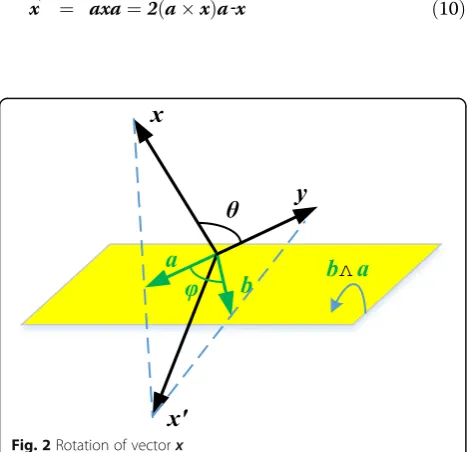
We will next introduce the rotor, one of the most im-portant objects in applications of geometric algebra. As
shown in Fig. 2, vector y is acquired through rotating
the vectorxwithθ. The rotation can be regarded as two consecutive reflections, first ina, then inb. Correspond-ingly, the expression that reflects x in the line with dir-ectionais
x0 ¼ axa¼2 að xÞa‐x ð10Þ
The expression appears to be strange at first, but it is actually one of the most important rationales why the geometric product is so useful.
Similarly,ycan be obtained by reflectingx’in the line with directionb
y¼bx0
b‐1¼baxa‐1b‐1¼ð Þbax bað Þ‐1 ¼ RxR‐1 ð11Þ
As shown in Eq. (11),Ris identified as the rotor. If we want to rotate a vector counterclockwise by a specific angle, we only need to apply the rotor to the vector. And, the rotation must be over twice the angle between aandb. In Appendix 1, a brief proof is given.
2.2 Complex representation matrix (CRM)
As stated above, we adopt multivector as a generic elem-ent of geometric algebra. However, the analysis of the mulitvector and its attendant theory are scarce. In view of this, we will introduce the CRM since the matrix the-ories are mature [14]. Similar to the multivector, we con-struct the matrix in geometric algebra, noted Gmn3 , as follows
with Im being the identity matrix of dimension m × m. Properties (14) and (15) can be verified by direct calculation using Eq. (16) and Eq. (17). For exyz
is isomorphic to complex imaginary unit j [9],
ψ(A)can be regarded as a complex matrix. Then, all the operation rules of the complex matrix are applic-able to ψ(A). Some properties [15] which will be used in the sequel are listed as follows.
a) A=B⇔ψ(A) =ψ(B);
b)ψ(A+B) =ψ(A) +ψ(B) ,ψ(AC) =ψ(A)ψ(C); c) ψ(A+) =ψ+(A).
It is also worthwhile to note that the following three properties regarding P2m and Q2m will be of use in the
forthcoming calculations.
d)P2mPþ2m¼Im;
e) Pþ2mP2mψð Þ ¼A ψð ÞA Pþ2nP2n;
f ) Q2m¼Qþ2m:
2.3 Manifold modeling of vector sensors in the conformal array
In this subsection, we will combine the electromagnetic vector sensors with the conformal array, and present a unified model based on geometric algebra to estimate the DOAs. To illustrate the versatility of this algorithm,
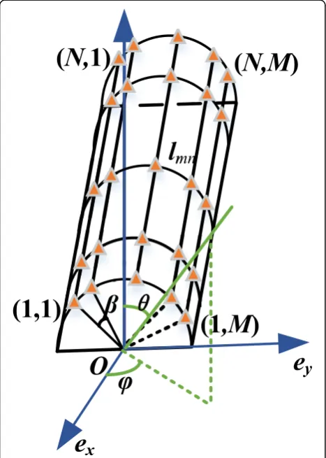
we consider a M × N cylindrical conformal array as
shown in Fig. 3. The array containsNuniformly spaced
rings on the surface. In addition, there are M
electro-magnetic vector sensors distributed on each ring. The angle between two consecutive elements on the same
ring is β. In addition, the radius of the cylinder and the
distance between adjacent rings are R and W,
respectively.
Since the electromagnetic vector sensor consists of six spatially collocated antennas, the three electric field components (Ex, Ey, Ez) and the three magnetic field
components (Hx. Hy, Hz) can be measured
simultan-eously. Thus, we can use two multivectors,XeandXh, to
represent the electric field signal and the magnetic field signal, respectively.
Xe¼ExexþEyeyþEzez ð18Þ
Xh¼HxexþHyeyþHzez ð19Þ
Similarly, the noise can be written as
Ne¼NExexþNEyeyþNEzez ð20Þ
Nh¼NHxexþNHyeyþNHzez ð21Þ
Then, the output of single element can be obtained in the frame of geometric algebra.
Y¼XeþexyzXhþNeþexyzNh ð22Þ
From (22), we see that exyz not only provides a vital
link between electric field components and magnetic field components, but also offers the possibility to han-dle the data model in geometric algebra. Due to the lim-ited length, the relationship between the two fields will be derived in Appendix 2. In addition, from (18, 19, 20, and 21), we see that the orthogonality of the signal com-ponents is reserved. Compared with the conventional methods, such as the long vector algorithm [8], this or-thogonality constraint implies stronger relationships be-tween the signal components. The proof can be seen in Appendix 3. And it is also the most important advantage of the output model. Using the Maxwell equations in the formalism of geometric algebra, Eq. (22) can be written in another shape.
Y¼ð1þuÞSEþNeþexyzNh ð23Þ
where
u¼ cosφsinθexþ sinφsinθeyþ cosθez ð24Þ
with u representing the unit vector of the signal propagation andSEbeing the complex envelope of the electric field. In addition, the signal has an elevation angle θ and an azimuth angle φ. The derivation of (23) is omitted here and the interested reader will find more material in [10].
Considering the polarization information, the afore-mentioned complex envelope,SE, can be written as
SE¼ΘhS ð25Þ
wherehis the signal polarization vector [16] and can be described by the auxiliary polarization angle (γ) and the polarization phase difference (η), that is, h¼
cosγ sinγeexyzη
½ T
. AndS is the multivector symboliz-ing the complex envelope of the signal. Moreover, the parameter Θ denotes the steering vector of the angle field [17] and is independent of the space location:
Θ¼
Thus, the polarized version of (23) can be expressed as
Y¼ð1þuÞΘhS
As stated above, the cylindrical conformal array is
composed ofM ×Nelements. In addition, suppose that
there areKnarrowband sources impinging on the array.
The manifold of the conformal array as shown in Fig. 3 corresponding to thekth source is
as θk; ;φk
ent pattern in the array global Cartesian coordinate sys-tem. In subsequent equations the range of m and n is the same and is omitted. Rmn and λk are the (m, n)th
element location vector and the kth signal wavelength respectively. The received signals of the array are the superposition of the response of each signal, the output can be expressed as
Y¼XK
k¼1
askXkþNy¼Aθk; ;φk; ;γk; ;ηk
SþNy ð29Þ
whereXkis a special case ofX regarding the kth source. And
S¼½S1 S2 ⋯ SKT ð30Þ
Ny¼ Ny1Ny2⋯NyK
T
ð31Þ
with Sk being the complex envelope of the kth signal. For notational convenience, we will simply write A in-stead ofA(θk, φk, γk,ηk) whenever there is no possibility
of confusion.
Let us refer back to Eq. (28). It is worthwhile to note that the aforementioned manifold of the conformal array,ask, is derived under the global coordinate system.
The azimuth and elevation angles are defined in Fig. 3. In most ready-made algorithms, the element pattern,
gmn(θk, φk), is always considered to be identical.
Never-theless, due to the effects of the curvature of conformal carriers, the above assumption is not satisfied in the cy-lindrical conformal array.
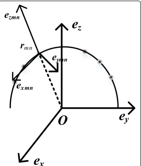
In what follows, we will use the rotor in geometric al-gebra to model the conformal array, together with the vector-sensor array. The most important advantage of geometric algebra in analyzing conformal arrays is that we are able to express the geometry and the physics in a coordinate-free language. As stated above, the rotor can be used to realize the rotation between the two coordin-ate systems. Thus, we define the local coordincoordin-ate system of the (m,n)th element as shown in Fig. 4.
The exmn axis is the same asex axis in the global
co-ordinate system, ezmn is perpendicular to the element
surface and eymn is tangent to the surface which can
form a standard Cartesian coordinate system. Then, transforming the global coordinate into the local one is
equivalent to rotating the global coordinate about ex
axis. The corresponding rotation angle is
ξ¼ðm−1Þβ−M−1
Substituting ez and ey for b and a, respectively (see
Appendix 1, the exponential form of the rotor), the rotor is
Rmn¼e‐ðez∧eyÞ
ξ
2 ð33Þ
Utilizing E3= exeyez as the pseudo-scalar in 3-D
Eu-clidean space, Eq. (33) can be further simplified
Rmn¼eE3exξ2 ð34Þ
Through (11), we can acquire the standard orthogonal basis in the local coordinate. And the specific procedure can refer to Appendix 4. We herein directly give the results
Thus, from (35, 36 and 37), we can obtain the element pattern,gmn(θk,φk).
Up to present, the remaining unknown variable is the location vector. From Fig. 3, we can obtain its specific expression
where δ means the spacing between adjacent rings. Then, the mainfold of the conformal vector-sensor array,
A, can be obtained.
Since the geometric algebra is introduced in modeling the manifold, the eigendecomposition is different from the conventional methods, such as [18]. In fact, similar to the quaternion case [19], the noncommutativity of the geometric product leads to two possible eigenvalues, namely the left and the right eigenvalue. However, in this paper, we select the right eigenvalue since the right
eigendecomposition of A can be converted to the right
eigendecomposition of the CRM. We construct the covariance matrix
RY ¼EfYYþg ¼AEfSSþgAþþ6σ2IMN ð39Þ
Here, we assume that the noise is identical and uncor-related from element to element, with covarianceσ2.
ForRYis a unitary matrix, its eigendecomposition can be written as
RY ¼UYsDYsUþYsþUYnDYnUþYn ð40Þ
Where UYs is the MNxKmatrix composed of the K
ei-genvectors corresponding to theKlargest eigenvalues of
RY, termed as the signal subspace. UYn represents the
matrix composed of the eigenvectors corresponding to
the 2 M–Ksmaller eigenvalues, i.e., the noise subspace. According to the principles of the MUSIC algorithm, the array manifold spans the signal subspace and is orthog-onal to the noise subspace. In this case, we have
AþU
Yn¼02M−K ð41Þ
where 02M−K is a 2 M–K row vector with all elements
equal zero. The proof can be seen in Appendix5.
In practice,RY ¼L1
Yn, the maximum likelihood estimation ofRY, is always used as the covariance matrix. Among which,Lrepresents the number of snapshots. In this case, (41) becomes
AþU
Yn≈02M−K ð42Þ
Up to present, the DOA estimation model of con-formal vector-sensor array has been established. This is also the focus of our paper. The contents of constructing the spatial spectra and searching the peak are omitted here. The readers can refer to literature [18]. It is worth-while to note that in introducing the rotor, the spatial lo-cation of the sensor is not required. Then, the proposed method can be easily extended to other arrays.
It is also worthwhile to note that {ex,ey,ez} is not only
the basis for the multivector in the vector-sensor array, but also represents the coordinate in the conformal array. And, it can be used for transformation between the global and the local coordinates with the help of the rotor. Under this circumstance, there are some links between those two arrays. The commonality is one of the motivations for es-tablishing a unified model to estimate the DOAs.
3 Complexity analysis
To better explain the superiority of the geometric alge-bra in modeling the conformal vector-sensor array, we will introduce the computational complexity from the standpoint of deriving the manifold. And, the computa-tional burden is evaluated in terms of the number of multiplications, additions, and transpositions.
To this end, we will briefly introduce the conventional methods of analysis based on Euler angle in this section. Generally, the transformations between the element local coordinates and the array global coordinates may be implemented by three continuous Euler rotations [3]. The specific rotation matrix can be expressed as
RðC;D;FÞ ¼Rxð ÞCRyð ÞDRzð ÞF
cosDcosF −cosDsinF −sinD cosCsinF−cosFsinCsinD cosCcosFþsinCsinDsinF −cosDsinC sinCsinFþcosCcosFsinD cosFsinC−cosCsinDsinF cosCcosD
2 4
3 5
ð43Þ
Euler rotation angles about ex axis, ey axis and ez axis.
The matrices Rx(C), Ry(D), and Rz(F) are the
corre-sponding Euler rotation matrices. It is noted that two successive Euler rotations are usually adequate to deal with the cylindrical conformal array. The third Euler ro-tation matrix is added here to cope with some irregular or special conformal arrays. Additionally, we know the rotation matrix is invertible from Eq. (43). Consequently, taking the inversion with respect toR(C,D,F), we have
cosDcosF cosCsinF−cosFsinCsinD sinCsinFþcosCcosFsinD
−cosDsinF cosCcosFþsinCsinDsinF cosFsinC−cosCsinDsinF
−sinD −cosDsinC cosCcosD
2 4
3 5
ð44Þ
Combining Eq. (43) with Eq. (44), it is not hard to find that
RðC;D;FÞ−1¼RðC;D;FÞT ð45Þ
Thus,R(C,D,F) is the so-called orthogonal matrix. In this case, transforming the local coordinate into the glo-bal one is equivalent to imposing the transposition/in-version with respect to the above rotation matrix. If we model the conformal array based on the Euler angle, three matrix multiplications and one matrix transpos-ition are required for each element.
In fact, the matrix operations are essentially the multi-plications and the additions between elements. To quan-tify this, the amounts of multiplications and additions of the two methods (i.e., the proposed method and the Eu-ler angle method) are calculated, respectively. The corre-sponding results are shown in Table 2. We assume that one matrix transposition is considered as one multiplica-tion or addimultiplica-tion operamultiplica-tion. And it is obvious that the multiplication between two 3 × 3 matrices involves 9 × 3 multiplications and 9 × 2 additions. For conveni-ence, the multiplication and the addition are collectively referred to as the operation. Then, Eq. (43) contains 2 × 9 × 3 + 2 × 9 × 2 operations. For the conformal
array consisting of M × N electromagnetic vector
sen-sors, the transformation between different coordinates
involves 91 × 6 × MN operations. Compared with the
Euler rotation angle, the proposed method effectively avoids the cumbersome matrix transformations. From Eqs. (35, 36, and 37), we know eymnand ezmn are
inde-pendent ofex. In addition,exmncan be obtained directly
from Eq. (35) without extra operations. Thus, Eqs. (35, 36 and 37), can be expressed as a 2 × 2 matrix. While using the rotor to establish the array manifold, the com-putational process is equivalent to a 2 × 2 matrix multi-plied by a 2 × 1 vector. In this case, the operations for each element involve four multiplications and two
additions. The total amount of operations is
6 × 6 ×MN. Thus, the geometric algebra-based method
significantly decreases the computational burden. In general, the Euler rotation and its matrix represen-tation cannot intuitively exhibit the complete procedure. In addition, as the configuration of the conformal array becomes more irregular and complex, the level of com-plexity involved in the transformations and the number of calculations required increases largely.
4 Simulation results
In this section, Monte-Carlo simulation experiments are used to verify the effectiveness of the proposed algo-rithm. The array structure is shown in Fig. 3. Among
which, we select M and Nas 4 and 4, respectively. The
angle between two consecutive elements on the same ring,β, is 5°. The number of snapshots,L, is 200. Under these premises, 200 independent simulation experiments are carried out. The root mean square error (RMSE) is utilized as the performance measure and is defined as
RMSE¼ azimuth angles, respectively, at theith run.
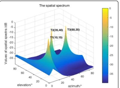
Provided that there are three polarized signals can be received. The incident angles are (10°, 15°), (35°, 40°),
and (60°, 35°), respectively. The corresponding
polarization auxiliary angles and the polarization phase differences are (15°, 25°), (30°, 45°), and (50°, 65°). Fig-ure 5 shows the simulation results of the proposed algo-rithm. The position of the spectrum peak represents the possible DOA. Intuitively, the estimation accuracy of the proposed algorithm is high.
To better demonstrate the performance of the pro-posed method, Qi’s method [3] and Gao’s algorithm [20] are included for comparison. We study the performance with a varying SNR from 0 to 30 dB. Without loss of generality, we select the first source(T1) and the second source (T2), respectively, to verify it. Figure 6 shows the RMSE versus SNR with the snapshots being 200. It can
be seen that the proposed method outperforms the Qi’s
information compared with the scalar array. Moreover, in contrast to those two algorithms, the proposed one effectively avoids the cumbersome matrix transforma-tions, and therefore, has a much lower computational complexity. It is noted that, for the statistical data have certain randomness, the simulation curve in Fig. 6 is not smooth.
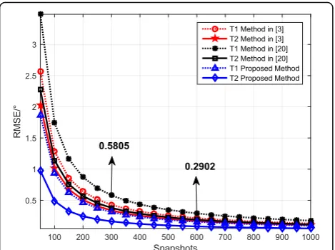
Figure 7 illustrates the RMSE versus the number of snapshots with the SNR fixed at 10 dB. Compared with Fig. 6, we can draw similar conclusions. In particular, if we pick the points with snapshots being 300 and 600, respect-ively, we may find that the corresponding RMSEs are 0.5805 and 0.2902. This means the former value is nearly twice as much as the latter one. In fact, these improve-ments can be predicted from the derivation of CRB. The specific derivation process can refer to literature [21]. The number of snapshots can be extracted from the Fisher in-formation matrix. Moreover, the CRB is found as the element of the inverse of that matrix. So, we can conclude that the RMSE is inversely proportional toL.
To better demonstrate the computational efficiency, the specific operations, such as the multiplications, addi-tions, and transposiaddi-tions, are simulated in Fig. 8. The value of thex-axis (or the abscissa) represents the product ofM and N. It can be seen that the multiplications take up the most resources. Compared with Euler rotation an-gles, the proposed method reduces the computation by one order of magnitude. Thus, the proposed algorithm provides the possibility for real-time processing.
5 Conclusions
In this correspondence, we combine the electromagnetic vector sensors with the conformal array, and present a unified model based on geometric algebra to estimate the DOAs. Compared with existing methods, the pro-posed one has two main advantages. Firstly, it can give a more accurate estimation by preserving the orthogonal-ity of the signal components. Secondly, it avoids the cumbersome matrix operations while performing the co-ordinate transformations, and therefore, has a much lower computational complexity. In addition, it has a strong commonality, that is to say, it is not limited to any specific conformal array. The simulation results ver-ify the effectiveness of the proposed method.
6 Appendix 1
6.1 Here we will give a brief proof to demonstrate that the rotation must be over twice the angle betweenaand
b
To proceed further, we rewriteRaccording to the defin-ition of the geometric product:
R¼ba¼b⋅aþb∧a ð47Þ
Here, we consider the case that the vectors are unit length. This assumption is reasonable, because the basic vectors of the Cartesian coordinate system satisfy it as well. The geometric product ofbʌaitself is:
Table 2The computational complexity of the proposed method and Euler angle
Multiplications Additions Transpositions Operations
Euler angle 2 × 9 × 3 × 6 ×MN 2 × 9 × 2 × 6 ×MN 6 ×MN 91 × 6 ×MN
Proposed method 4 × 6 ×MN 2 × 6 ×MN 0 6 × 6 ×MN
b∧a
ð Þðb∧aÞ ¼ðba‐b⋅aÞðb⋅a‐abÞ ¼b•a bað þabÞ‐ðb⋅aÞ2‐baab
¼b⋅að2b⋅aÞ‐ðb⋅aÞ2‐b aað Þb
¼ðb⋅aÞ2‐bb
¼cos2θ‐1
¼‐sin2θ
ð48Þ
Thus, we define the 2-bladeE2:
E2¼ b∧a
sinθ ð49Þ
Rcan be further simplified by substituting (49) into (47):
R¼ cosθ‐E2sinθ ð50Þ
The expression is similar to the polar decomposition of a complex number with the unit imaginary replaced by the 2-bladeE2. (50) can also be written as the
expo-nentials ofE2:
R¼e‐E2θ ð51Þ
This formalism is more useful for the log-space of ro-tors is linear. We split x into a part (xp) parallel to bʌ
a-plane and a part (xo) orthogonal tobʌ a-plane. Then,
xois not affected by the applicationR. And we infer that
the rotation must be in thebʌa-plane. As stated above, the rotation consists of two successive reflections which are orthogonal (angle-preserving) transformations. Thus, it allows us to pick any vector in the bʌ a-plane to de-termine the angle. Without loss of generality, we choose vector a, and construct the “sandwich product” RaR−1 as shown in (11):
RaR‐1¼baaa‐1b‐1¼bab‐1 ð52Þ
where bab−1 is the reflection of a in b. From this it is clear that the rotation must be over twice the angle be-tween a and b, since the angle between a and bab−1is twice the angle betweenaandb. The negative signature in (51) represents the rotation direction.
7 Appendix 2
7.1 We demonstrate howexyzlinks the electric field with the magnetic field
First, let us refer back to the famous Maxwell equations described by the vector algebra are
∇Ε¼‐μ∂∂H
t ð53Þ
∇⋅Ε¼ρ
ε ð54Þ
∇Η ¼ε∂∂E
t ð55Þ
∇⋅Η ¼0 ð56Þ
where E=Exex+Eyey+Ezez and H=Hxex+Hyey+Hzez
are, respectively, the electric and magnetic fields. In addition, the parameters ε, μ, and ρ symbolize the
Fig. 7RMSE versus snapshots with the SNR fixed at 10 dB
permittivity, the permeability, and the density of the source charges, respectively.
It is worthwhile to give some results before proceeding to the physical problems of interest:
x∧y¼exyzxy ð57Þ
Using Eqs. (57, 58 and 59), the Maxwell equations in geometric algebra can be expressed as follows:
∇∧Εþμ∂∂H
Since the arriving signals are assumed to be far-field, so the signals received on different positions differ only by a transmission delay, that is,
E r;ð tÞ ¼Eð0;t‐τÞ ð64Þ
withc representing the propagation speed andu denot-ing the signal propagation as defined in (24). Let
Eð Þ ¼t Eð0;tÞ ¼Exð Þt exþEyð Þt eyþEzð Þt ez ð67Þ
Hð Þ ¼t Hð0;tÞ ¼Hxð Þt exþHyð Þt eyþHzð Þt ez ð68Þ
Then,
E r;ð tÞ ¼Eð Þt‐τ ð69Þ
H r;ð tÞ ¼Hð Þt‐τ ð70Þ
For plane waves, we know
∇¼u
c ∂
∂t ð71Þ
Substituting Eqs. (67, 68, 69, 70 and 71) into Maxwell equations, we have addition, combining the geometric implication of the inner product with Eq. (74), we knowEð Þt is the orthog-onal complement ofu in the plane Hð Þt exyz. That is to say, Eð Þt anduare orthogonal in that plane. Thus, the
parameter ρ in (73) equals to zero. Then, Eqs. (72, 73)
are equivalent to Eqs. (74, 75). We rewrite (73), u
c⋅E
t
ð Þ ¼0 ð76Þ
Combining (72) and (76), we have ffiffiffi
denotes the intrinsic impedance of the medium.
Integrating (77) with respect to timet, ffiffiffi
whereq is a constant and equals to zero in the far-field assumption.
Up to this point, we have derived how exyz links the
electric field with the magnetic field.
8 Appendix 3
8.1 We show the orthogonality constraint implies stronger relationships between the signal components Consider two electric field multivectors Xe1, Xe2, with
their expressions given by
Xe1¼Ex1exþEy1eyþEz1ez ð79Þ
Xe2¼Ex2exþEy2eyþEz2ez ð80Þ
By imposing the orthogonality for the two
multivectors
Xe2; Xe1
h ig ¼XHe1⋅Xe2¼0 ð81Þ
where 〈⋅〉g represents the inner product in geometric algebra.
EHx1Ex2þEHy1Ey2þEHz1Ez2¼0 ð82Þ
Ex2EHy1¼Ey2EHx1 ð83Þ
Ey2EHz1¼Ez2EHy1 ð84Þ
Ex2EHz1¼Ez2EHx1 ð85Þ
However, for long vector algorithm, the
multivec-tors are replaced by the vecmultivec-tors xe1, xe2, and
Similarly, imposing the orthogonality for the two vectors
xe2; xe1
h iv¼xH
e1⋅xe2¼0 ð87Þ
where〈⋅〉vdenotes the inner product between two vectors.
We can get the same result as in (82). However, Eqs. (83, 84 and 85) cannot be obtained. In other words, using geometric algebra to model the output imposes stronger constraints between the compo-nents of the vector sensor array.
9 Appendix 4
9.1 The detailed calculation procedures of Eqs. (35, 36 and 37), are given as follows. Since the derivations of Eqs. (36, 37) are similar to that of Eq. (35), we will take Eq. (35) as an example. And the other two equations can be obtained similarly. The derivation of (35) is
exmn¼RmnexRmn‐1
10.1 We will verify the rationality of Eq. (41)
Using property (b) and Eq. (39), we can obtain the CRM ofRY, that is
SinceRsis full rank, it is easy to obtain
rankfψð ÞAψð ÞRs ψþð ÞA g ¼K ð91Þ
According to the principle of MUSIC, we have
ψþð ÞA U
ψn¼02Kð2M−KÞ ð92Þ
Where Uψn∈G32Mð2M−KÞ composed of the eigenvectors
corresponding to the 2 M–K smaller eigenvalues of
ψ(RY). Using the property (d), Eq. (92) is equivalent to
the following equation.
P2KPþ2Kψ
þð ÞA U
ψn¼02Kð2M−KÞ ð93Þ
By means of the property (e), Eq. (93) can be further expressed as
ψþð ÞA Pþ
2MP2MUψn¼02Kð2M−KÞ ð94Þ
Taking the multiplication on the left byP2K, we have
AþU
Yn¼0Kð2M−KÞ ð95Þ
Where UYn¼P2MUψn∈G3Mð2M−KÞ is composed of the
ei-genvectors corresponding to the 2 M–K smaller eigen-values ofRY. Thus, Eq. (41) holds.
Acknowledgements
The authors would like to thank the anonymous reviewers for the improvement of this paper.
Funding
This project was supported by the National Natural Science Foundation of China (Grant No.61302017).
Authors’contributions
Tianzhen MENG conceived the basic idea and designed the numerical simulations. Minjie WU analyzed the simulation results. Naichang YUAN refined the whole manuscript. All authors read and approved the final manuscript.
Competing interests
The authors declare that they have no competing interests.
Publisher’s Note
Received: 31 March 2017 Accepted: 6 September 2017
References
1. Lu Gan, Xiaoyu Luo. Direction-of-arrival estimation for uncorrelated and coherent signals in the presence of multipath propagation, IET Microwaves, Antennas & Propagation, 2013, vol. 7, no. 9, pp. 746-753, DOI: https://doi. org/10.1049/iet-map.2012.0659
2. Lars Josefsson, Patrik Persson. Conformal Array Antenna Theory and Design, IEEE Press Series on Electromagnetic Wave Theory, 2006, ISBN:978–0– 471-46584-3
3. Z. -S. Qi., Y., Guo., B. -H. Wang. Blind direction-of-arrival estimation algorithm for conformal array antenna with respect to polarisation diversity, IET Microwaves, Antennas & Propagation, 2011, vol. 5, no. 4, pp. 433-442, DOI: https://doi.org/10.1049/iet-map.2010.0166
4. B. H. Wang, Y. Guo, Y. L. Wang, Y. Z. Lin. Frequency-invariant pattern synthesis of conformal array antenna with low corss-polarisation, IET Microwaves, Antennas & Propagation, 2008, vol. 2, no. 5, pp. 442-450, ISSN: 1751-8725, DOI:https://doi.org/10.1049/iet-map:20070258
5. P. Alinezhad, S.R. Seydnejad, D. Abbasi-Moghadam, DOA estimation in conformal arrays based on the nested array principles. Digit. Signal Process. 50, 191–202 (2016). https://doi.org/10.1016/j.dsp.2015.12.009
6. L. Zou, J. Lasenby, Z. He, Pattern analysis of conformal array based on geometric algebra, IET Microwaves, Antennas & Propagation, 2011, vol. 5, no. 10, p. 1210-1218, ISSN: 1751-8725, DOI: https://doi.org/10.1049/iet-map.2010.0588 7. W.U. Minjie, Z.H.A.N.G. Xiaofa, H.U.A.N.G. Jingjian, Y.U.A.N. Naichang, DOA
estimation of cylindrical conformal array based on geometric algebra. Int J Antennas Propagation2016, 1–9 (2016). https://doi.org/10.1155/2016/7832475 8. A. Nehorai, E. Paldi, Vector-sensor array processing for electromagnetic
source localization. IEEE Trans. Signal Process.42(2), 376–398 (1994). https:// doi.org/10.1109/78.275610
9. N.L. Bihan, S. Miron, J. Mars, MUSIC algorithm for vector-sensors array using biquaternions. IEEE Trans. Signal Process.55(9), 4523–4533 (2007). https:// doi.org/10.1109/TSP.2007.896067
10. J.F. Jiang, J.Q. Zhang, Geometric algebra of euclidean 3-space for electromagnetic vector-sensor array processing, part I: modeling. IEEE Trans. Antennas Propag.58(12), 3961–3973 (2010). https://doi.org/10.1109/TAP. 2010.2078468
11. Venzo De Sabbata, Bidyut Kumar Datta. Geometric Algebra and Applications to Physics. CRC Press, 2007, ISBN: 978-1-58488-772-0
12. J.W. Arthur,Understanding geometric algebra for electromagnetic theory(IEEE Press, New Jersey, 2011) ISBN: 978-1-118-07854-3
13. Dietmar Hildenbrand. Foundations of geometric algebra computing, 2013, Springer, ISBN: 978–3–642-31793-4, DOI: https://doi.org/10.1007/978-3-642-31794-1
14. Leo Dorst, Daniel Fontijne, Stephen Mann. Geometric Algebra for Computer Science, 2007, Morgan Kaufmann, ISBN: 978-0-12-369465-2
15. John Snygg. A New Approach to Differential Geometry Using Clifford’s Geometric Algebra, Birkhäuser, 2010, New York, ISBN: 978-0-8176-8282-8 16. DESCHAMPS G. A. Techniques for handling elliptically polarized waves with
special reference to antennas: part II-geometrical representation of the polarization of a plane electromagnetic wave. Proc. IRE, 1951, vol. 39, p. 540-544. DOI:https://doi.org/10.1109/JRPROC.1951.233136
17. W.U. Minjie, Y.U.A.N. Naichang, DOA estimation in solving mixed non-circular and non-circular incident signals based on the non-circular array. Prog. Electromagn. Res. M53, 141–151 (2017). https://doi.org/10.2528/ PIERM16092105
18. R. Schmidt, Multiple emitter location and signal parameter estimation. IEEE Trans. Antennas Propag.AP-34(3), 276–280. ISSN: 0018-926X (1986). https:// doi.org/10.1109/TAP.1986.1143830
19. S. Miron, N.L. Bihan, J.I. Mars, Quaternion-MUSIC for vector-sensor array processing. IEEE Trans. Signal Process.54(4), 1218–1229 (2006). https://doi. org/10.1109/TSP.2006.870630
20. Ziyang Gao, Yong Xiao. Direction of arrival estimation for conformal arrays with diverse polarizations, 2015 12thIEEE International Conference on
Electronic Measurement & Instruments, pp. 439–442. DOI: https://doi.org/10. 1109/ICEMI.2015.7494229