DOI: 10.1534/genetics.106.063149
A Maximum-Likelihood Method for the Estimation of
Pairwise Relatedness in Structured Populations
Amy D. Anderson
1and Bruce S. Weir
Department of Biostatistics, University of Washington, Seattle, Washington 98195
Manuscript received July 10, 2006 Accepted for publication February 16, 2007
ABSTRACT
A maximum-likelihood estimator for pairwise relatedness is presented for the situation in which the individuals under consideration come from a large outbred subpopulation of the population for which allele frequencies are known. We demonstrate via simulations that a variety of commonly used estimators that do not take this kind of misspecification of allele frequencies into account will systematically overes-timate the degree of relatedness between two individuals from a subpopulation. A maximum-likelihood estimator that includesFSTas a parameter is introduced with the goal of producing the relatedness es-timates that would have been obtained if the subpopulation allele frequencies had been known. This estimator is shown to work quite well, even when the value ofFSTis misspecified. Bootstrap confidence intervals are also examined and shown to exhibit close to nominal coverage when FST is correctly specified.
T
HE use of molecular marker data to infer the degree of relatedness between two individuals is of in-terest in a variety of contexts (see Weiret al. 2006 for a review). Several estimators have been developed for the case in which the loci are unlinked and the individuals are not inbred. These include Thompson’s maximum-likelihood estimator (Thompson1975; Milligan2003) and a variety of other estimators (e.g., Queller and Goodnight1989; Liet al. 1993; Ritland1996; Lynch and Ritland1999; Wang2002).The above methods generally assume that allele fre-quencies are known without error, but Wang (2002) also considered the case in which allele frequencies were estimated from a sample of sizeNfrom the popu-lation in which relatedness is to be estimated. In this work, we consider a different situation: the case in which the individuals examined belong to a subpopu-lation of the popusubpopu-lation to which known allele frequen-cies apply. An example of this situation would be when ‘‘European’’ allele frequencies are used in estimating the relatedness between two individuals who happen to be Italian.
The effect of using allele frequencies from the overall population is to shift the reference from which we mea-sure relatedness back in time. As an illustration, con-sider the case in which two individuals share copies of an allele that is common in their subpopulation, but very rare in the population as a whole. Using the subpopu-lation allele frequencies, the fact that both individuals
have this allele provides little evidence for relatedness. When the population allele frequencies are used, however, the evidence for relatedness becomes strong. The difference is that, when the population allele fre-quencies are used, relatedness is implicitly measured with respect to the time when the population allele fre-quencies held in the subpopulation, that is, before the subpopulation split from the ancestral population (which may be assumed to have allele frequencies similar to that of the current overall population—there is an implicit assumption here that the overall population is so large that its allele frequencies remain roughly unchanged over time). In this scenario, the relatedness estimate us-ing the population allele frequencies is affected by the generations during which the allele frequencies in the subpopulation were diverging via drift from that in the overall population. From that perspective, the abun-dant copies of the allele in the subpopulation may all be copies of one allele in the ancestral population and these two individuals both have copies because they share common ancestry. Hence, even though the indi-viduals may not be closely related with respect to recent generations, the fact that they share alleles that are rare in the overall population provides evidence that they may be closely related with respect to their more distant ancestry. The difference in allele frequencies between the subpopulation and the overall population is itself suggestive of relatedness between the individuals: Both are consequences of finite population size.
In contrast to the estimate of relatedness found by ap-plying population allele frequencies, the estimate using the subpopulation allele frequencies ignores the evolu-tionary history during which the allele frequencies in the 1Corresponding author: Department of Biostatistics, University of
Washington, F-600 Health Sciences Bldg., Campus Mail Stop 357232, Seattle, WA 98195-7232. E-mail: [email protected]
subpopulation drifted to their current states. Hence, this estimate measures relatedness relative to the period of time when the current subpopulation allele frequencies began to (approximately) hold.
Depending on a researcher’s particular interests, he or she may prefer the estimate from using the overall population frequencies or that obtained from the sub-population frequencies. The choice would depend upon the timescale of the researcher’s scientific question.
As an example, suppose a researcher was interested in estimating rates of extrapair paternity in some species of birds. This is inherently a question of relatedness in just the preceding generation—whether a mother bird’s social mate is in fact the father of her offspring or, if the mother’s social mate is unavailable for testing, a ques-tion of whether her chicks are full or half siblings. From the perspective of this researcher, blindly using the pop-ulation allele frequencies would inflate the degree of relatedness between the individuals (by including evo-lutionary relatedness that is irrelevant to this study).
On the other hand, if a species is in danger of extinc-tion, a researcher might be interested in determining the relatedness between individuals to determine which individuals might be bred with each other to maximize the genetic diversity maintained in the population. In this case, if the researcher is interested in creating a population with maximum heterozygosity, he or she is concerned with relatedness going back for many gen-erations and so might prefer to use the population allele frequencies and an estimation procedure that takes inbreeding into account.
The methodology in this article is relevant to the first of these researchers: We present a methodology for estimating the degree of relatedness between individu-als that would have been obtained had the researcher been able to use current subpopulation allele frequen-cies instead of the overall population frequenfrequen-cies.
To create such an estimator, we need to be able to characterize the variation between the allele frequencies in a subpopulation and those in the overall population. This variation between allele frequencies between two or more populations can be summarized by the popula-tion structure parameter,u(also known asFST). Balding and Nichols(1997) estimateduusing data from studies performed by Krane et al. (1992) and Budowle and Monson (1994) in which mixed Caucasian allele fre-quencies at variable number tandem repeat (VNTR) loci were compared to allele frequencies in various Euro-pean subpopulations (e.g., Norway, Spain, Turkey). They examined three loci in each data set and found that, for the six loci examined,uwas generally,0.01, although at one locus larger values ofu could not be ruled out. Weir (1994) estimated a common u-value for Apache, Navajo, and Pima populations using allele frequencies calculated from a pool of the three populations and obtained values of 0.02, 0.041, 0.097, 0.032, and 0.111 at the five VNTR loci considered. In a more recent study,
Weiret al. (2005) estimatedu using two large SNP data sets. The HapMap data set (International HapMap Consortium2005) contained data on four human sub-populations: Caucasians of European descent, Yoruba from Ibadan, Nigeria, Han Chinese from Beijing, and Japanese from Tokyo. The genomewide estimate of
u using all four of these populations was 0.13. The Perlegen (Hindset al. 2005) data set, which contained European Americans, African Americans, and Han Chinese from the Los Angeles area, yielded 0.10 as an estimate ofu.
Values ofuestimated for animal populations are often even higher. Kretzmannet al. (2003) considered sam-ples from five subpopulations of the Egyptian vulture (Neophron percnopterus) from the Iberian peninsula, Canary Islands, and Balearic Islands. They used geno-types at nine microsatellite loci to estimateu-values be-tween pairs of the populations (or, in the language of this work, they estimated a commonufor each pair of subpopulations, using the allele frequencies estimated from a pool of the two samples). Of the 10 pairwise
u-estimates, 3 were,0.015, 3 were between 0.05 and 0.1, 3 were between 0.1 and 0.15, and 1 was 0.295. In a similar study, Marshall and Ritland (2002) used 10 micro-satellite loci to examine the genetic differentiation among 11 subpopulations of black bear (Ursus americanus) in the Pacific Northwest. Of the 55 pairwise u-estimates from this study, 5 were,0.05, 28 were between 0.05 and 0.10, 18 were between 0.10 and 0.15, and 4 were$0.15.
In this article, we apply a maximum-likelihood ap-proach to relationship estimation, based upon a gener-alization of Thompson’s (1976) likelihood in which we account for population structure by includinguin our model. This model is the same as that given in Ayres (2000), but, whereas Ayres used the model to present formulas for some specific likelihood ratios, we present the likelihood equations in their general form and use them to find maximum-likelihood estimators.
THEORY AND METHODS
In this section, we begin by outlining the likelihood method developed by Thompson (1975). In notation we follow the treatment given in Milligan(2003): Our Table 1 and Figure 1 are essentially identical to those in Milligan’s article. We then proceed to explain the model we use to describe the relationship between allele fre-quencies in the subpopulation and those in the ancestral population and, using this model, derive the likelihood analogous to that of Thompson.
speak of relationship estimation, we generally refer to the estimation of one or more parameters related to the probability that alleles are shared IBD between two in-dividuals. One such parameter is the coancestry coef-ficient, uXY, which represents the probability that an allele chosen at random from individualXis IBD to an allele chosen at random from individualY. An equiva-lent parameter is the relatedness coefficient,r¼2uXY.
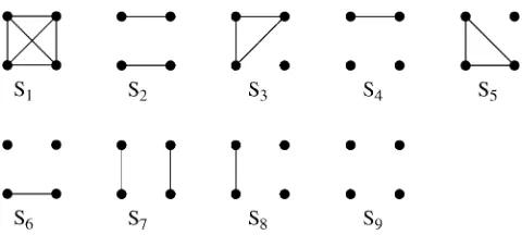
Jacquard(1972) described a set of nine identity-by-descent modes that give a full description of the possible IBD relationships between the set of four alleles pos-sessed by two (possibly inbred) individuals. These are denoted S1;. . .;S9 and are shown in Figure 1. The probability that a pair of individuals will be in IBD mode Siis denotedDi.
As an example, if two noninbred individuals are full siblings (that is, they share both a mother and a father and the mother and father are unrelated), thenD7¼ 0.25,D8¼0.5, andD9¼0.25. All other IBD modes are impossible for noninbred full siblings. Indeed, all IBD modes other thanS7,S8, andS9can occur only if one or both of the two individuals are inbred.
If it is assumed that two related individuals are not inbred, then only three IBD modes are possible:S7,S8, andS9. These can be described more simply by noting the number of alleles shared IBD between the two
individuals. IBD mode S7 corresponds to the case in which two alleles are shared IBD between the two in-dividuals, whereasS8andS9correspond to the sharing of one and zero alleles, respectively. In this case, the relevant probabilities,D7,D8, andD9correspond to the probabilities that the pair share two, one, and zero al-leles, respectively, and are often denoted byk2,k1, and
k0. Note thatk21k11k0¼1.
It is usually not possible to look at the alleles in two individuals and infer their IBD mode. We can, however, tell which alleles are identical by state (IBS), that is, which alleles share the same allelic type. There are 9 IBS modes, denotedS1;. . .;S9, and these are listed in the ‘‘Allelic state’’ column in Table 1.
The genetic information about the relationship be-tween two individuals that can be found using unlinked loci pertains exclusively to the estimation of the pro-portion of loci in the genome that are in each IBD state. Hence, with unlinked loci, two relationships with iden-tical single-locus IBD probabilities are indistinguishable. As an example, noninbred half-sibling, grandparent– grandchild, and avuncular relationships all havek0¼0.5,
k1¼0.5, andk2¼0.0, so it is impossible to distinguish between these relationship types with unlinked loci.
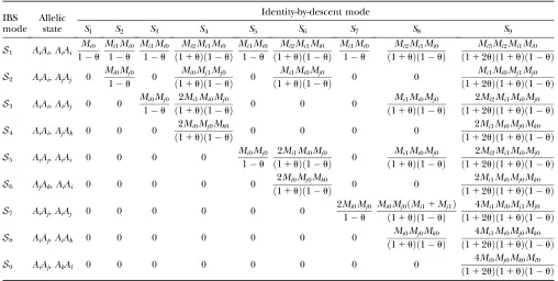
Thompson’s model: Thompson (1975) assumed a model in which the individuals under consideration came from a single population in Hardy–Weinberg equi-librium. In such a situation, two random alleles that are not IBD may be considered to be two random draws from the population of alleles. Under this assumption, the probabilities of observing each of the nine possible IBS modes, conditioned on the IBD mode, are shown in Table 1. Using these probabilities, the single-locus like-lihood of a relationship specified by D, between two individuals whose IBS mode isSi, can be found by
con-ditioning on the IBD mode as follows: LðDÞ ¼PrðSijDÞ ¼
X
j
PrðSijSjÞDj: ð1Þ Multilocus likelihoods for unlinked loci are formed by taking the product of the single-locus likelihoods. Figure 1.—Jacquard’s identity-by-descent modes. Each
group of four dots represents an IBD mode between two dividuals. The top pair of dots represents the two alleles in in-dividual 1 and the bottom pair of dots represents the two alleles in individual 2. Lines connect alleles that are IBD.
TABLE 1
Probabilities for various identity-by-state modes, given modes of identity-by-descent
IBS mode
Allelic state
Identity-by-descent modeSj
S1 S2 S3 S4 S5 S6 S7 S8 S9
S1 AiAi,AiAi pi pi2 p 2 i p
3
i p 2 i p
3
i p 2 i p
3
i p 4 i
S2 AiAi,AjAj 0 pipj 0 pipj 0 p2ipj 0 0 pi2p 2 j
S3 AiAi,AiAj 0 0 pipj 2pi2pj 0 0 0 pi2pj 2pi3pj
S4 AiAi,AjAk 0 0 0 2pipjpk 0 0 0 0 2pi2pjpk
S5 AiAj,AiAi 0 0 0 0 pipj 2pi2pj 0 pi2pj 2pi3pj
S6 AjAk,AiAi 0 0 0 0 0 2pipjpk 0 0 2pi2pjpk
S7 AiAj,AiAj 0 0 0 0 0 0 2pipj pipj(pi1pj) 4pi2p 2 j
S8 AiAj,AiAk 0 0 0 0 0 0 0 pipjpk 4pi2pjpk
S9 AiAj,AkAl 0 0 0 0 0 0 0 0 4pipjpkpl
Thompson (1975) used these likelihood equations primarily for the purpose of constructing likelihood ra-tios to compare the probability of the observed marker data under two competing hypotheses concerning the re-lationship between the individuals. Milligan (2003) used the likelihood to estimatek2,k1, andk0and hence obtain an estimate foruXY¼ 0.5k21 0.25k1. He then compared the performance of the maximum-likelihood estimator to the performance of various method-of-moments estimators.
Model with population substructure:Unlike Thomp-son’s model, in which the individuals come from a single panmictic population with the given allele frequencies, we consider the case in which individuals come from a subpopulation of the population for which allele fre-quencies are known. For populations in equilibrium and loci for which the postmutation state of an allele is independent of its premutation state, it has been shown (Wright1951; Griffiths1979) that allele frequencies among the subpopulations follow a Dirichlet distribu-tion. Under similar assumptions, Baldingand Nichols (1994) derived equations for joint allele probabilities within a subpopulation using the population allele fre-quencies; these results match the moments of a Dirich-let distribution.
The Dirichlet distribution depends upon the pop-ulation structure parameter described above. This pa-rameter,u, can be thought of as a correlation among alleles in the subpopulation: The probability that the first allele drawn from the population isAispA(because,
although we do not know the allele frequencies specific to the subpopulation, we do know that the expected al-lele frequency in the subpopulation is the same as the population allele frequencypA) and, given that the first
allele drawn wasA, the probability that the second allele drawn will also beAispA1u(1pA). The equilibrium
assumption means thatuis not changing over time. One can also think of u as an IBD probability. The current population allele frequencies approximate those of an ancestral population from which the subpopulation descended. When we estimate IBD using the subpopu-lation allele frequencies, we use Thompson’s model in which IBD is measured with respect to some previous generation when the current subpopulation allele fre-quencies held. Using the population allele frefre-quencies forces our frame of reference back to the ancestral pop-ulation. Two alleles that are merely IBS with respect to the subpopulation model may be IBD when the longer population history is taken into account. In this context,
urepresents the probability that any two alleles in the subpopulation are IBD with respect to the ancestral population.
In Thompson’s model, two individuals have a re-lationship specified byDand alleles that are not IBD are considered to be drawn independently at random ac-cording to the subpopulation allele frequencies. Using population allele frequencies instead of subpopulation
frequencies forces us to consider the subpopulation alleles within a longer evolutionary framework, where our ‘‘not IBD’’ alleles are no longer drawn independently because they may be IBD to previously seen alleles when IBD is measured with respect to the ancestral population. To calculate the likelihood under a model in which the subpopulations are related to the overall population with population structure parameteru, we first note that Equation 1 still holds, but the calculation of PrðSijSjÞ
will now be undertaken under the assumption that our individuals belong to a subpopulation of the population from which the allele frequencies apply.
Under the Dirichlet model, joint probabilities for sets of alleles can be calculated as described, for example, in Weir (2003). In particular, if (p1, p2, . . ., pn) are the population allele frequencies of allelesA1,. . .,An, at a
locus, the probability that a sample of alleles from the subpopulation will containt1alleles of typeA1,t2alleles of typeA2, and so forth, is given by
Prðt1;. . .;tnÞ ¼C
GðgÞ
Gðg1tÞ
Y
i
Gðgi1tiÞ
GðgiÞ ; ð2Þ
whereGindicates the usual gamma function,gi¼(1u) pi/u, g¼
P
igi¼ ð1uÞ=u, and C is a constant
in-dicating the number of possible orderings in which we could have drawn a sample with these allele counts.
DefineMi,j¼[(1u)pi1ju], fori¼1, 2,. . .andj¼0,
1,. . .. Suppose the single-locus joint genotype,g, of two individuals containstialleles of typeAi(soti2{0, 1, 2,
3, 4}), and let h denote the number of heterozygous individuals in the pair (soh2{0, 1, 2}). Then
PrðgÞ ¼ 2
hQ i
Qti1 j¼0 Mi;j Q2n1
j¼0 ½11ðj1Þu
: ð3Þ
Table 2 shows the probabilities of the nine possible joint IBS states given the nine possible IBD states. Note that, whenu¼0, these reduce to the probabilities given in Table 1. Using these probabilities, the likelihood can be calculated as in Equation 1. In determining the maximum-likelihood estimator, we considerD1,. . .,D9, which refer to IBD probabilities measured with respect to the subpopulation, to be parameters whileu, which measures the background IBD that comes from the relationship between the subpopulation and the ances-tral population, is considered to be a known constant. As in Thompson’s model, we assume that genotypes at dis-tinct unlinked loci are independent and, hence, the multilocus likelihood is the product of the single-locus likelihoods.
Parameter space: In the analyses presented in this article, we consider the case in which the subpopulation is large and outbred. In this case,D1¼. . .¼D6¼0 and the likelihood is a function ofk0,k1, andk2. It is also true that, in an outbred population, the IBD parameters k2, k1, and k0are subject to the constraint 4k2k0 , k21 (Thompson1976), and we have incorporated this con-straint into our estimations. Our parameter space is then {k2,k1,k0: 0#ki#1 (i¼0, 1, 2),k01k11k2¼1, 4k2k0,k12}. To find the maximum-likelihood estimator for the coancestry coefficient,uXY, for a pair of individuals, we
first use the simplex method (Presset al. 2002) to find maximum-likelihood estimators fork2,k1, andk0 and then estimate ˆuXY ¼0:5ˆk210:25ˆk1.
Other estimators: In this article, we compare our maximum-likelihood estimator to various other popular relationship estimators. These include the maximum-likelihood estimator described by Thompson (1975) and Milligan(2003), as well as a number of other esti-mators that we briefly describe below.
The Queller–Goodnight (QG) estimator, first intro-duced in Queller and Goodnight (1989), is one of the earlier relationship estimators. We chose to use the form of the Queller–Goodnight estimator presented in Equation 11 of Lynchand Ritland(1999), where we averaged the single-locus estimates across loci. The simi-larity index (SIM) (Liet al. 1993) is another popular re-lationship estimator. Here, we use the version given in Equation 8 of Lynch and Ritland (1999), averaged
across loci. The Lynch–Ritland (LR) estimator is known to perform well and is given in Equations 5–7 of Lynch and Ritland (1999), with a weighted average taken across loci. The final moment estimator we use is Wang’s estimator, which we denote as W and compute accord-ing to Equations 9 and 10 in Wang(2002).
Both the QG and LR estimators are asymmetric with respect to the two individuals, that is, ˆuXY 6¼uˆYX. For
these two estimators, we use the average of the estimates taken from the different orderings of the two individuals. Assessing uncertainty in the estimators: An estima-tion of relatedness is incomplete without an indicaestima-tion of the uncertainty associated with that estimation. Suppose mmarkers were genotyped in the two individuals being compared. A different estimate of relatedness might occur if a different set ofmmarkers had been chosen. If we think of our set of markers as being randomly chosen from some distribution of possible markers, we want a confidence interval such that a fixed proportion (e.g., 95%) of all random sets of mmarkers would produce intervals that contain the true parameter value. To do this, we created bootstrap confidence intervals for the estimates, where bootstrapping was done over loci. More specifically, each bootstrap sample consisted of the two individuals’ genotypes atm loci, where the loci in the bootstrap sample are chosen at random (with replace-ment) from the originally genotypedmloci. Each boot-strap sample yielded an estimate for ˆuXY, and the final 95% confidence interval for the original pair of
TABLE 2
Probabilities for various identity-by-state modes, given modes of identity-by-descent when the individuals being compared belong to a subpopulation of the population from which the allele frequencies are estimated
IBS mode
Allelic state
Identity-by-descent mode
S1 S2 S3 S4 S5 S6 S7 S8 S9
S1 AiAi,AiAi
Mi0 1u
Mi1Mi0 1u
Mi1Mi0 1u
Mi2Mi1Mi0
ð11uÞð1uÞ Mi1Mi0
1u
Mi2Mi1Mi0
ð11uÞð1uÞ
Mi1Mi0 1u
Mi2Mi1Mi0
ð11uÞð1uÞ
Mi3Mi2Mi1Mi0
ð112uÞð11uÞð1uÞ S2 AiAi,AjAj 0
Mi0Mj0 1u 0
Mi0Mj1Mj0
ð11uÞð1uÞ 0
Mi1Mi0Mj0
ð11uÞð1uÞ 0 0
Mi1Mi0Mj1Mj0
ð112uÞð11uÞð1uÞ S3 AiAi,AiAj 0 0
Mi0Mj0 1u
2Mi1Mi0Mj0
ð11uÞð1uÞ 0 0 0
Mi1Mi0Mj0
ð11uÞð1uÞ
2Mi2Mi1Mi0Mj0
ð112uÞð11uÞð1uÞ S4 AiAi,AjAk 0 0 0
2Mi0Mj0Mk0
ð11uÞð1uÞ 0 0 0 0
2Mi1Mi0Mj0Mk0
ð112uÞð11uÞð1uÞ S5 AiAj,AiAi 0 0 0 0
Mi0Mj0 1u
2Mi1Mi0Mj0
ð11uÞð1uÞ 0
Mi1Mi0Mj0
ð11uÞð1uÞ
2Mi2Mi1Mi0Mj0
ð112uÞð11uÞð1uÞ
S6 AjAk,AiAi 0 0 0 0 0
2Mi0Mj0Mk0
ð11uÞð1uÞ 0 0
2Mi1Mi0Mj0Mk0
ð112uÞð11uÞð1uÞ
S7 AiAj,AiAj 0 0 0 0 0 0
2Mi0Mj0 1u
Mi0Mj0ðMi11Mj1Þ
ð11uÞð1uÞ
4Mi1Mi0Mj1Mj0
ð112uÞð11uÞð1uÞ
S8 AiAj,AiAk 0 0 0 0 0 0 0
Mi0Mj0Mk0
ð11uÞð1uÞ
4Mi1Mi0Mj0Mk0
ð112uÞð11uÞð1uÞ
S9 AiAj,AkAl 0 0 0 0 0 0 0 0
4Mi0Mj0Mk0Ml0
ð112uÞð11uÞð1uÞ
individuals was found by taking the middle 95% of the estimates from the bootstrap samples.
Simulations: We ran a series of simulations in which we compared the performance of the various point esti-mators under a variety of circumstances. Each simula-tion began with the generasimula-tion of allele frequencies for the overall population, and allele frequencies in the subpopulation were stochastically generated from these using the Dirichlet distribution as described, for exam-ple, in Weir(2003). In our analyses, we used the allele frequencies from the ancestral population in estimating the relatedness between individuals in subpopulations. In our first set of simulations, we considered an ancestral population with 10 markers, each of which had 10 alleles with frequencies determined by a triangle distribution. For each value ofu(u¼0.0, 0.03, 0.10), we generated 4000 sets of subpopulation allele frequencies, and, for each of these subpopulations, we estimated the relatedness of 1000 pairs of individuals of each of the following types: parent–offspring (PO), full sibling (FS), half sibling (HS), first cousins (FC), second cousins (SC), and unrelated (UN). The genotypes for relative pairs were generated using the subpopulation allele frequencies and the appropriate IBD probabilities (k0,
k1,k2) for the relationship type. In these simulations, we estimated the bias and root mean-square error (RMSE) for each subpopulation and then presented the average of these values across subpopulations.
For the second set of simulations, we were interested in the behavior of the various estimators within a sub-population and whether the maximum-likelihood estima-tor was sensitive to misspecification ofu. All simulations were performed with 10 markers, each with 10 alleles. For each value ofu(u¼0.0, 0.03, 0.10), we generated a set of subpopulation allele frequencies and simulated 1000 pairs of individuals of each relationship type using these frequencies. We estimated the MLE using various assumed values ofu(u¼0.0, 0.01, 0.02, 0.03, 0.05, 0.10, 0.15) and also obtained relatedness estimates from the moment estimators. To get a sense of whether our re-sults would vary substantially depending on either the allele frequencies in the ancestral population or the particular realization of subpopulation allele frequen-cies, we carried out the analysis on five replicate sub-populations for each of the following types of allele frequencies in the ancestral population: equally fre-quent alleles, triangle allele frequencies, and random allele frequencies generated from a Dirichlet distribu-tion with all parameters set to unity. Once we had de-termined that our results did not vary substantially among these simulations, we ran larger data sets of 5000 relative pairs of each type from subpopulations (u¼0.0, 0.03, 0.10) of a population in which the overall allele frequencies followed a triangle distribution.
The third set of simulations was designed to in-vestigate the effect of varying the number and type of loci. We considered both diallelic and microsatellite (10
alleles) loci and varied the number of loci from 5 to 100. For both marker types, the ancestral population had triangle allele frequencies. In the case in which loci were diallelic, the QG estimator is undefined for heterozy-gous individuals, so we did not consider its performance in these simulations. In addition, in the situation with diallelic loci, if all loci have equal assumed allele fre-quencies, the SIM and Wang estimators are identical, so we presented only one of these in our results. For each combination of number of loci, number of alleles, and
u, we simulated 10,000 relative pairs of each type (full sibling and unrelated).
We also performed a set of simulations to investigate the performance of bootstrap confidence intervals for the fMLE. In these simulations, we looked at one sub-population of an overall sub-population in which each locus had 10 alleles with frequencies determined by a triangle distribution and considered cases in which 5, 10, 15, 20, 30, and 40 loci were used. Within the subpopulation, we generated 1000 relative pairs of each type, and for each pair we used 1000 bootstrap samples of the markers to determine a 95% confidence interval. We also ran a series of simulations to examine the behavior of the con-fidence intervals for varying assumed values ofu. In this series of simulations, for each combination ofu(u¼0.00, 0.03, 0.10) and number of markers (10 or 40), we sim-ulated 1000 relative pairs from a single simsim-ulated sub-population and then formed a bootstrap confidence interval for each relative pair under several assumed values ofu. When the data were simulated underu¼0.00, we analyzed the data with each of the following assumed values of u: 0.00, 0.01, 0.03, and 0.05. When the true value ofuwas 0.03, the data were analyzed underu¼0.00, 0.01, 0.03, 0.05, and 0.08. Whenu ¼0.10, we analyzed the data assumingu¼0.05, 0.08, 0.10, 0.12, and 0.15.
different pairs of relatives may have an effect on the in-terpretation of our results. In particular, this depen-dence will not bias the relatedness estimates for any given family, but we would expect the mean estimates from each family to vary more than if they were based on independent relative pairs.
The allele frequencies we used were those listed in the CEPH data sets, with one exception: Any allele whose allele frequency was listed as zero in the CEPH data set but appeared in that data set was reassigned an allele frequency of 13104.
RESULTS
Simulation results: Figure 2 shows the average bias and RMSE over subpopulations descended from a pop-ulation that had 10 alleles at each of 10 loci considered. We first compared the performance of the rMLE and moment estimators to examine their robustness to this type of model misspecification. The moment estimators all performed similarly and all showed increasing bias with increasing values ofu. The rMLE also increases its bias with increasingu, but not as severely as the moment estimators. When u is as large as 0.10, the moment estimators no longer show less bias than the rMLE.
We next examined how the bias and RMSE would be affected by using a model that takes population structure into account. In all cases, the fMLE showed reduced bias compared to models that do not take population struc-ture into account. Even when we use the true value of
u in the fMLE, though, the bias still increased withu. Naturally, though, this bias will be seen to decrease when the number of loci increases.
A plot corresponding to Figure 2 was also produced for the case in which the overall population had all alleles equally frequent, but was similar to the triangle
allele-frequency case and so is not shown here. The main dif-ference between the existing Figure 2 and the version with equally frequent alleles is the relative performance of the moment estimators.
Figure 3 shows a more in-depth view of the results from a single subpopulation. As before, we considered 10 loci, each with 10 alleles that had triangle allele frequencies in the overall population. We performed these simula-tions under three values of u and compared the four moment estimators as well as maximum-likelihood esti-mators under various assumed values ofu. The top row of Figure 3 shows the behavior of the estimators when there is no population structure. The plot showing the relatedness estimates for unrelated individuals clearly demonstrates a fundamental difference between the moment and maximum-likelihood estimators: The mo-ment estimators can give relatedness estimates that are less than zero whereas the maximum-likelihood esti-mates are constrained to give results that lie within the space of possible values for u. Note that, for distantly related or unrelated individuals, this constraint causes much of the bias seen in the maximum-likelihood esti-mators: Since it is impossible for the estimator to sub-stantially underestimate the degree of relatedness, but it is possible to overestimate this value, the estimator will, on average, overestimate the degree of relatedness. The unbiasedness of the moment estimators is a result of the undesirable property of allowing estimates that are less than zero. A comparison of the box plots of the actual esti-mates shows the superior performance of the maximum-likelihood estimator.
The second and third rows of plots in Figure 3 show the effects of increasing the degree of population struc-ture. The results confirm what was seen in Figure 2: Ignoring population structure causes inflation in the relationship estimates, and this effect is reduced when Figure 2.—Average behavior in
we account for the population structure in our likelihood. In addition, we see that the MLE calculated from the likelihood with population structure is quite robust to misspecification ofu. In particular, analyzing the data with a specified value ofuthat is a little too high may actually improve the performance (by helping to counter some of the natural bias in the MLE).
In Figures 4 and 5, we examined the effect of number and type of loci for estimating the relatedness of full siblings and unrelated pairs of individuals drawn from one subpopulation. In each case, we show the mean pa-rameter estimate and RMSE from 10,000 relative pairs. For full siblings, we see that, although accounting for population structure reduces the bias associated with the estimators, it provides little reduction in the RMSE unlessuis large. For unrelated pairs, however, the MLE
that takes population structure into account shows a notable reduction in RMSE compared to the other esti-mators for all values ofuexamined. Figures 4 and 5 also illustrate the point that increasing the number of loci does not necessarily result in increased accuracy when the allele frequencies are misspecified.
Looking at the behavior of each estimator for un-related pairs of individuals can give insight into how the various estimators respond to this type of model mis-specification. The fMLE approaches zero as the number of loci are increased. The models that do not account for population structure naturally measure relatedness relative to some ancestral population. The parameteru
is the probability that any two alleles drawn from the subpopulation are IBD with respect to that ancestral population. Hence, we might expect an estimator that Figure3.—Box plots showing the distribution of the estimators on a single subpopulation. We simulated 5000 relative pairs of
does not take population structure into account to have a nonzero expected value ofufor ‘‘unrelated’’ individ-uals. However, under the assumption that any two alleles have a nonzero probability of being IBD, all nine of Jacquard’s IBD configurations are possible, so the estimators under consideration (which assume no in-breeding) also have to contend with this type of model misspecification.
For unrelated individuals, as the number of loci increases, the rMLE appears to approach the value of
uused to simulate the data, but we have not looked into its behavior closely. The moment estimators display a variety of behaviors. In the appendix, we derive the expected behavior of the moment estimators as a func-tion ofuin the general diallelic case and in the case in which there arenequally frequent alleles at a locus. In the diallelic case, Wang’s estimator has an expected value of u/2 whereas the Lynch–Ritland estimator hasu/(11u) as its expected value. In the case withn equally frequent alleles, the Lynch–Ritland and Queller– Goodnight estimators are identical and have an ex-pected value ofu/(11u), regardless of the value ofn. The similarity index and Wang’s estimator have expected values that depend onnand approachu/(11u) andu(1 13uu2)/(113u12u2), respectively, asn/‘.
Bootstrap simulation results: Figures 6 and 7 show Monte Carlo estimates for the coverage probabilities of bootstrap 95% confidence intervals for the rMLE and
fMLE, respectively. When population structure is not taken into account (Figure 6), coverage decreases with increased sample size. When the data are analyzed under the correct model, however, the coverage for all relationships examined and all values of u was at least 88.5% whenever at least 10 loci were used (results not shown). In Figure 7, we see the effects of misspecifying the value ofuassumed in the analysis. For small sample sizes, this method of constructing confidence intervals is robust to misspecification of u. When the number of markers is large, however, the fact that these confidence intervals do not take uncertainty in u into account results in reduced coverage, especially for more dis-tantly related individuals.
CEPH results: Figures 8 and 9 show the mean esti-mates and root mean-square error for the relative pairs of each type (parent–offspring, full siblings, grandparent– grandchild, unrelated) within the CEPH data set for the initial set of 49 markers with gene diversities between 0.7 and 08. The Utah families, where we would expect
u to be small, show a pattern similar to that seen in our simulated data sets with little or no population structure: All estimators show fairly little bias, with the maximum-likelihood estimators generally exhibiting lower RMSE than the other estimators. Figure 10 shows the mean estimates using the second set of 49 markers.
Although there is some variation between the various families and between marker sets, the MLE does not give Figure 4.—Full siblings.
mean results that are substantially different from the non-maximum-likelihood estimators for the Utah fam-ilies. In other words, 49 unlinked markers seem to be enough to make the MLE (with u ¼ 0) essentially unbiased.
In the Amish family, relative pairs show inflated re-latedness estimates, especially among the grandparent– grandchild and unrelated pairs. The Old Order Amish
form a small genetic isolate, so any pair of individuals from this population may be expected to share multiple ancestors in recent generations. Thus, a relative pair from this group will often be more related than the nominal degree of relatedness indicated in the CEPH pedigrees. The genealogy of this particular Amish family is known for more generations than are included in the CEPH database and none of the grandparents in Figure 5.—Unrelateds.
Here, we have generated 10,000 pairs of unrelated in-dividuals from a single sub-population and examined the effect of the number of loci and number of possible alleles on relationship esti-mation. The symbols for the various estimators are as given in Figure 2.
Figure 6.—Coverage probabilities based on
the CEPH pedigree share common ancestors within the three preceding generations (Egeland1972; Broman and Weber1999). Nevertheless, with both our marker sets, the mean maximum-likelihood estimate for re-latedness for each type of relative pair was higher than the nominal level, even when we alloweduto be as high as 0.05.
A previous study (Broman and Weber 1999) has shown evidence of excess relatedness (as evidenced by exceptionally long spans of homozygosity within individ-uals) within the Venezuelan family (CEPH family 102). Because of this and the fact that Venezuelan allele fre-quencies might well be quite different from the Utah al-lele frequencies that should have dominated the CEPH allele frequency estimates, we expected the Venezuelan families to show higher than nominal degrees of
re-latedness, especially with the non-maximum-likelihood estimators. Contrary to our expectations, though, all re-latedness estimators performed well for this family using both sets of markers.
A close look at the RMSE values in the various families indicates that the Amish and Venezuelan families differ from the Utah families in an important way. As an over-all principle, increasing the value ofuused in the MLE calculations decreases the estimated coancestry coeffi-cient between a pair of individuals. For pairs of un-related individuals, then, it is clear that increasing the value ofuwill always result in a decrease in RMSE. When highly polymorphic markers are used, the same is also true for parent–offspring pairs for the following reason: When two individuals share at least one allele at a marker, the single-locus MLE for the coancestry coefficient at that Figure7.—Effects of parameter
misspe-cification on confidence interval coverage. Each plot shows the empirical coverage probabilities for bootstrap confidence in-tervals based on a fixed number of markers (10 or 40) and a set degree of population structure (u ¼ 0.00, 0.03, 0.10). Within each plot, for each type of relative pair is the coverage of 95% confidence intervals based on 1000 pairs of individuals, where the analysis was performed under various assumed values ofu. When the true value ofuwas 0.00, we analyzed each pair of in-dividuals under the assumed values of (left to right) u ¼ 0.00, 0.01, 0.03, and 0.05. When the true value ofuwas 0.03, we ana-lyzed the data under assumed values ofu¼
0.00, 0.01, 0.03, 0.05, and 0.08. Finally, whenuwas 0.10, we performed analyses un-der assumed values ofu¼0.05, 0.08, 0.10, 0.12, and 0.15. In all cases, the results when the true value ofuwas assumed are repre-sented by a solid circle. All other values ofu are indicated by open circles.
Figure 8.—Mean estimates for the
CEPH data set, based on the first set of 49 loci. The families are denoted as follows:
marker will always be 0.25 or 0.5 unless the pair shares an allele with a population allele frequency.0.25. With highly polymorphic markers, we only rarely see alleles with such high frequencies. Hence, since the maximum-likelihood estimator for several markers should not be less than the minimum of the single-locus MLEs, we see that 0.25 is a lower bound for the MLE for the coancestry coefficient between a parent–offspring pair (note that this is not true for SNP markers as seen in Figure 4 of Weir et al. 2006). An increase in u thus results in a reduction of the RMSE for such pairs. For other relation-ships, increasingupast a certain point will drive the MLE below the correct value and cause an increase in the RMSE. For the Utah families, we see that increasingufor full siblings and grandparent–grandchild pairs always increases the RMSE, as might be expected if the true value ofuis small. The Amish family shows the opposite
pattern: Increasing u decreases the RMSE. This is consistent with two scenarios: The value ofuis truly very high or the individuals are truly more closely related than the nominal level. For the Venezuelan siblings, the minimum RMSE (among the u-values examined) is achieved whenu¼0.02.
DISCUSSION
Our purpose here has been to develop methodology for estimating relatedness within a subpopulation of a population in which allele frequencies are known or estimated. In effect, this method measures IBD proba-bilities with respect to recent generations while filtering out additional allele sharing that comes from the more distant generations during which allele frequencies in the subpopulation drifted to their current values.
Figure9.—Root mean-square error for
the CEPH data set, based on the first set of 40 loci. The symbols for this plot are the same as those in Figure 8.
Figure 10.—Mean estimates for the
The bottom left-hand plot in Figure 5 illustrates this point. Here, u ¼ 0.10 and the rMLE and other non-maximum-likelihood estimators estimate the relatedness of supposed unrelated individuals in this population at 0.10. From the perspective of the researcher interested in relatedness going back many generations, this is the correct answer:urepresents the degree of relatedness in the individuals relative to approximately the gener-ation when the subpopulgener-ation split from the overall population. For a researcher interested in questions regarding relatedness relative to less distant generations (specifically, the degree of relatedness that would be estimated if the researcher had access to allele fre-quencies from the subpopulation), the correct value for these unrelated individuals isuXY¼0, the value given by the fMLE.
We have looked at relatedness estimation from the perspective of researchers who want to base their esti-mators on the subpopulation allele frequencies but have access only to population allele frequencies. We have shown that this misspecification of allele frequen-cies causes positive bias in relatedness estimators that are currently in use. When the subpopulation is quite differentiated from the overall population, as is fre-quently seen in animal populations, the amount of the degree of bias can be large (for unrelated individuals, the expected amount of bias is approximately equal to the degree of differentiation between the subpopula-tion and the overall populasubpopula-tion).
We have proposed a maximum-likelihood estimator that takes population structure into account, but re-quires the degree of differentiation between the sub-population and the overall sub-population (uorFST) to be specified. Our simulations show that this estimator ex-hibits reduced bias compared to the estimators that ignore the possibility that allele frequencies come from an overall population rather than from the pertinent subpopulation. In addition, we have demonstrated that this estimator is fairly robust to small misspecifications ofu. Note that the value ofuused with this estimator will need to be estimated from a data set that does not contain individuals whose relatedness is in question be-cause u cannot be estimated from sets of individuals with unspecified relationships. Indeed, commonly used estimators for u (e.g., Weir and Cockerham 1984) require that it be estimated from data sets consisting of unrelated individuals from various subpopulations.
When we examined the effect of the number of loci on this full-model MLE, we saw that the functional rela-tionship between mean estimate (or RMSE) and num-ber of markers is shaped like a negative exponential. Hence, when few markers are being used, small in-creases in the number of markers produce large de-creases in bias and RMSE. When the number of markers is larger, though, it takes the addition of many more markers to give a substantial improvement in the esti-mator. Our simulation results indicate that, for highly
polymorphic markers such as microsatellites, moderate increases in the number of loci beyond, say, 40 or 60 has little effect. For diallelic loci (e.g., SNPs) substantial im-provements in performance are obtained at.100 loci. We did not pursue this beyond 100 loci because the methods presented here are for unlinked loci (where, by unlinked, we mean segregating independently within a single meiosis), and a genome will not contain many more than 50 such loci. We have reason to believe that maximum-likelihood estimation may be fairly robust to this assumption provided that the loci cover a wide region of the genome: Hepler (2005) performed maximum-likelihood estimation of Jacquard’s nine Delta parame-ters (D1,. . .,D9), using a large set of tightly linked loci spread over an entire human chromosome, and ob-tained quite accurate results.
To give a measure of confidence in our estimates, we proposed forming bootstrap confidence intervals for our estimates, where the bootstrapping is performed over the loci. When population structure exists and is not taken into account, we showed that the performance of these confidence intervals (as measured by their cover-age probabilities) decreased dramatically with increasing numbers of loci. When population structure was taken into account by using the full-model MLE with the correct value ofu, the confidence intervals performed well whenever the number of loci was . 10. With larger sample sizes, though, the performance of the con-fidence intervals depended on the specification ofu; a reduction in coverage occurred when analyses were per-formed with incorrect values of u. Not unsurprisingly, the greater the number of markers, the closer the as-sumed value ofuneeded to be to the true value for the confidence intervals to maintain adequate coverage.
We concluded our study by looking at the perfor-mance of various estimators based on 49 unlinked (or loosely linked) microsatellite loci genotyped on the eight CEPH reference families. Six of the families were from Utah and, for these, we would expect to have u
close to 0. Hence, this amounted to a comparison of pre-vious methods on a real data set. With 49 loci, all esti-mators were essentially unbiased and the MLE was shown to outperform the others in terms of RMSE (by virtue of performing better on parent–offspring and un-related pairs and performing no worse on full siblings and grandparent–grandchild pairs).
This work was supported in part by National Institutes of Health grants GM45344 and GM75091.
LITERATURE CITED
Ayres, K. L., 2000 Relatedness testing in subdivided populations. Forensic Sci. Int.114:107–115.
Balding, D. J., and R. A. Nichols, 1994 DNA profile match prob-ability calculation: how to allow for population stratification, re-latedness, database selection and single bands. Forensic Sci. Int. 64:125–140.
Broman, K. W., and J. L. Weber, 1999 Long homozygous chro-mosomal segments in reference families from the Centre d’E` tude du Polymorphisme Humain. Am. J. Hum. Genet.65: 1493–1500.
Budowle, B., and K. L. Monson, 1994 Greater differences in foren-sic DNA profile frequencies estimated from racial groups than from ethnic subgroups. Clin. Chim. Acta228:3–18.
Egeland, J. A. (Editor), 1972 Descendents of Christian Fisher and Other Amish-Mennonite Pioneer Families. Johns Hopkins Hospital, Baltimore.
Griffiths, R. C., 1979 A transition density expansion for a multial-lele diffusion model. Adv. Appl. Probab.11:310–325.
Hepler, A. B., 2005 Improving forensic identification using Bayes-ian networks and relatedness estimation. Ph.D. Thesis, North Carolina State University, Raleigh, NC.
Hinds, D., L. Stuve, G. Nilsen, E. Halperin, E. Eskin et al., 2005 Whole-genome patterns of common DNA variation in three human populations. Science307:1072–1079.
InternationalHapMapConsortium, 2005 A haplotype map of the human genome. Nature437:1299–1320.
Jacquard, A., 1972 Genetic information given by a relative. Biomet-rics28:1101–1114.
Krane, D. E., R. W. Allen, S. A. Sawyer, D. A. Petrovand D. L. Hartl, 1992 Genetic differences at four DNA typing loci in Finnish, Italian, and mixed Caucasian populations. Proc. Natl. Acad. Sci. USA89:10583–10587.
Kretzmann, M. B., N. Capote, B. Bautschi, J. A. Godoy, J. A. Dona´ zaret al., 2003 Genetically distinct island populations of the Egyptian vulture (Neophron percnopterus). Conserv. Genet. 4:697–706.
Li, C. C., D. E. Weeks and A. Chakravarti, 1993 Similarity of DNA fingerprints due to chance and relatedness. Hum. Hered. 43:45–52.
Lynch, M., and K. Ritland, 1999 Estimation of pairwise relatedness with molecular markers. Genetics152:1753–1766.
Marshall, H. D., and K. Ritland, 2002 Genetic diversity and dif-ferentiation of Kermode bear populations. Mol. Ecol.11:685– 697.
Milligan, B. G., 2003 Maximum-likelihood estimation of related-ness. Genetics163:1153–1167.
Press, W. H., S. A. Teukolsky, W. T. Vetterlingand B. P. Flannery, 2002 Numerical Recipes in C11: The Art of Scientific Computing, Ed. 2. Cambridge University Press, Cambridge, UK.
Queller, D. C., and K. F. Goodnight, 1989 Estimating relatedness using genetic markers. Evolution43:258–275.
Ritland, K., 1996 Estimators for pairwise relatedness and inbreed-ing coefficients. Genet. Res.67:175–186.
Thompson, E. A., 1975 The estimation of pairwise relationships. Ann. Hum. Genet.39:173–188.
Thompson, E. A., 1976 A restriction on the space of genetic relation-ships. Ann. Hum. Genet.40:201–204.
Wang, J., 2002 An estimator for pairwise relatedness using molecu-lar markers. Genetics160:1203–1215.
Weir, B. S., 1994 The effects of inbreeding on forensic calculations. Annu. Rev. Genet.28:597–621.
Weir, B. S., 2003 Forensics, pp. 830–852 inHandbook of Statistical Ge-netics, edited by D. Balding, M. Bishopand C. Cannings. John Wiley & Sons, Chichester, UK.
Weir, B. S., and C. C. Cockerham, 1984 Estimating F-statistics for analysis of population-structure. Evolution38:1358–1370. Weir, B. S., L. R. Cardon, A. D. Anderson, D. M. Nielsenand W. G.
Hill, 2005 Measures of human population structure show het-erogeneity among genomic regions. Genome Res.15:1468–1476. Weir, B. S., A. D. Andersonand A. B. Hepler, 2006 Genetic related-ness analysis: modern data and new challenges. Nat. Rev. Genet.7: 771–780.
Wright, S., 1951 The genetical structure of populations. Ann. Eu-gen.15:323–354.
Communicating editor: J. B. Walsh
APPENDIX
Here we derive the expected values of the Wang, Lynch–Ritland, similarity index, and Queller–Goodnight estimators for the general diallelic case and the case in which there arenequally frequent alleles at a locus. This is done for the situation in which the relative pair is drawn from a subpopulation of the population from which the allele frequencies are taken and the estimators are not modified to take this into account. The relative pairs in these calculations are not inbred except through the background relatedness, u, so their relatedness within the sub-population can be summarized by the values ofk0,k1, andk2.
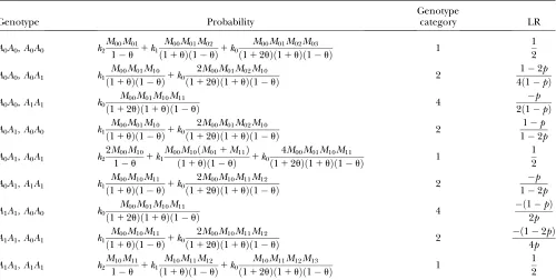
Wang’s estimator:Wang’s estimator (Wang2002) is based on the proportion of loci for which the relative pair is in each of four IBS categories. Category 1 includes any case in which the two individuals share two alleles IBS, category 2 includes cases in which three of the four alleles are IBS, category 3 consists of genotype pairs of the typeAiAj,AiAk, where
each ofAi,Aj, andAkrepresents a distinct allele, and category 4 contains any genotype pair for which the two individuals
share no alleles identical in state.Pidenotes the proportion of loci for which the relative pair falls into categoryi. Wang
adopts the following notational convention:ai¼
P
jp j i.
In the diallelic case, Wang’s Equation 8 implies the following:
ˆ
uXY ¼
4P1ˆ 13P2ˆ 2ð11a2Þ
4ð1a2Þ : ðA1Þ
Joint genotype probabilities for the diallelic case are given in Table A1. The expected values ofPˆ1andPˆ2are as follows:
E½P1ˆ ¼Pr½A0A0;A0A01Pr½A0A1;A0A11Pr½A1A1;A1A1 ¼k21k1M00M011M10M11
ð1uÞ
1k0
M00M01M02M0314M00M01M10M111M10M11M12M13
E½P2ˆ ¼k12M00M10
ð1uÞ 1k0
4M00M01M02M1014M00M10M11M12
ð112uÞð11uÞð1uÞ : ðA3Þ
At a single locus, the expected value of ˆuXY is
E½uˆXY ¼
4E½Pˆ113E½Pˆ2 2ð11a2Þ 4ð1a2Þ
¼ 1
4p0p1
2k21k12M00M01
12M10M1113M00M10
ð1uÞ
12k0
1
ð112uÞð11uÞð1uÞðM00M01M02M0314M00M01M10M11
1M10M11M12M1313M00M10M11M1213M00M01M02M10Þ 2ð1p0p1Þ
¼ 1
4p0p1
½2k21k1ð2p0p11up0p1Þ12k0ð1p0p11up0p1Þ 2ð1p0p1Þ
¼ 1
4p0p1
½2up0p112k2p0p1ð1uÞ1k1p0p1ð1uÞ
¼u
21ð1uÞ 2k21k1
4
¼u
21ð1uÞuXY:
ðA4Þ
For multiple loci, Wang replaces each ofPˆ1,Pˆ2, andaa2in Equation A1 with a weighted average of its value across all loci. The expected value ofE½uˆXYremains the same as that in the single-locus case.
Note that, whenu¼0 (as it is in Wang’s model), the estimator is unbiased foruXY. Whenu.0, however, we might
expect that an estimator that does not take population structure into account might have the property thatE½uˆXY ¼u
for unrelated individuals. Wang’s estimator instead givesE½ˆuXY ¼u=2 for diallelic loci in this case.
For the case in which the locus hasn equally frequent alleles, Table A2 lists the possible IBS modes and their probabilities. Note that, with all alleles equally frequent,Mij¼M0jfor alliandj. Since each IBS mode corresponds to
TABLE A1
Joint genotype probabilities for diallelic loci for individuals that are not inbred except for background inbreeding captured byu
Genotype Probability
Genotype
category LR
A0A0,A0A0 k2
M00M01 1u 1k1
M00M01M02
ð11uÞð1uÞ1k0
M00M01M02M03
ð112uÞð11uÞð1uÞ 1
1 2
A0A0,A0A1 k1
M00M01M10
ð11uÞð1uÞ1k0
2M00M01M02M10
ð112uÞð11uÞð1uÞ 2
12p
4ð1pÞ A0A0,A1A1 k0
M00M01M10M11
ð112uÞð11uÞð1uÞ 4
p
2ð1pÞ A0A1,A0A0 k1
M00M01M10
ð11uÞð1uÞ1k0
2M00M01M02M10
ð112uÞð11uÞð1uÞ 2
1p
12p A0A1,A0A1 k2
2M00M10 1u 1k1
M00M10ðM011M11Þ
ð11uÞð1uÞ 1k0
4M00M01M10M11
ð112uÞð11uÞð1uÞ 1
1 2
A0A1,A1A1 k1
M00M10M11
ð11uÞð1uÞ1k0
2M00M10M11M12
ð112uÞð11uÞð1uÞ 2
p
12p A1A1,A0A0 k0
M00M01M10M11
ð112uÞð11uÞð1uÞ 4
ð1pÞ
2p A1A1,A0A1 k1
M00M10M11
ð11uÞð1uÞ1k0
2M00M10M11M12
ð112uÞð11uÞð1uÞ 2
ð12pÞ
4p A1A1,A1A1 k2
M10M11 1u 1k1
M10M11M12
ð11uÞð1uÞ1k0
M10M11M12M13
ð112uÞð11uÞð1uÞ 1
several genotypes, we have also listed the number of genotypes included in each IBS mode. For example, if there aren alleles, there arengenotypes of the form (AiAi,AiAi).
The expected values ofP1,P2, andP3are
E½Pˆ1 ¼k21k1
nM00M01ð11uÞ ð11uÞð1uÞ 1k0
nM00M01ðM02M0312ðn1ÞM00M01Þ
ð112uÞð11uÞð1uÞ ðA5Þ
E½P2ˆ ¼k12nðn1ÞM002M01
ð11uÞð1uÞ 1k0
4nðn1ÞM002M01M02
ð112uÞð11uÞð1uÞ ðA6Þ
E½P3ˆ ¼k1nðn1Þðn2ÞM003
ð11uÞð1uÞ 1k0
4nðn1Þðn2ÞM003M01
ð112uÞð11uÞð1uÞ : ðA7Þ
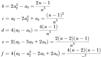
Wang’s equations for the multiallelic case are written in terms of some functions of the allele frequencies. These functions, and their values in the equally frequent allele case, are as follows:
b¼2a22a4¼2n1
n3 c¼a22a221a4¼ðn1Þ
2 n3 d ¼4ða3a4Þ ¼4ðn1Þ
n3
e¼2ða23a312a4Þ ¼2ðn2Þðn1Þ
n3
f ¼4a2a222a312a4¼4ðn2Þðn1Þ
n3
TABLE A2
Joint genotype probabilities for general loci when all loci havenequally frequent alleles
IBS mode Count Probability
Genotype
category LR SXY SIM
AiAi,AiAi n k2
M00M01 1u 1k1
M00M01M02
ð11uÞð1uÞ1k0
M00M01M02M03
ð112uÞð11uÞð1uÞ 1
1
2 1
1 2
AiAi,AiAj n(n1) k1
M2 00M01
ð11uÞð1uÞ1k0
2M2 00M01M02
ð112uÞð11uÞð1uÞ 2
n2 4ðn1Þ
3 4
ð3n2Þðn2Þ
8ðn1Þ2
AiAi,AjAj n(n1) k0
M2 00M
2 01
ð112uÞð11uÞð1uÞ 4
1 2ðn1Þ 0
12n
2ðn1Þ2 AiAi,AjAk
nðn1Þðn2Þ
2 k0
2M3 00M01
ð112uÞð11uÞð1uÞ 4
1 2ðn1Þ 0
12n
2ðn1Þ2
AiAj,AiAi n(n1) k1
M2 00M01
ð11uÞð1uÞ1k0
2M2 00M01M02
ð112uÞð11uÞð1uÞ 2
1 2
3 4
ð3n2Þðn2Þ
8ðn1Þ2
AiAj,AiAj
nðn1Þ
2 k2
2M2 00 1u1k1
2M2 00M01
ð11uÞð1uÞ1k0
4M2 00M
2 01
ð112uÞð11uÞð1uÞ 1
1
2 1
1 2
AiAj,AiAk n(n1)(n2) k1
M3 00
ð11uÞð1uÞ1k0
4M3 00M01
ð112uÞð11uÞð1uÞ 3
n4 4ðn2Þ
1 2
n24n12 4ðn1Þ2
AiAj,AkAk
nðn1Þðn2Þ
2 k0
2M3 00M01
ð112uÞð11uÞð1uÞ 4
1
n2 0
12n
2ðn1Þ2 AiAj,AkAl
nðn1Þðn2Þðn3Þ
4 k0
4M4 00
ð112uÞð11uÞð1uÞ 4
1
n2 0
12n
g ¼17a214a22110a38a4¼ðn4Þðn2Þðn1Þ
n3 V ¼ ð1bÞ2ð
e2f 1dg2Þ ð1bÞðef dgÞ212
cdfð1bÞðg1eÞ1c2dfðd1fÞ ¼4ðn1Þ
5ðn2Þ n13 ðn
3n21n2Þðn23n13Þ:
Wang writes equations for ˆk1 and ˆk2(which he denotes ˆfand ˆD) in terms of the above functions. Using Wang’s Equations 9 and 10, the expected values of the estimates ofk1andk2are
E½ˆk1 ¼E½fdf½ðe1gÞð1bÞ1cðd1fÞðP1ˆ 1Þ1dð1bÞ½gð1bdÞ1fðc1eÞP3ˆ 1fð1bÞ½eð1bfÞ1dðc1gÞP2ˆ g=V
¼ 1
V
16ðn1Þ4ðn2Þðn23n13Þ
n10 ðE½P1ˆ 1Þ
18ðn1Þ
4ðn2Þðn23n13Þðn21n1Þ
n11 E½P2ˆ
14ðn1Þ
4ðn2Þðn23n13Þðn21n1Þ
n11 E½P3ˆ
¼E½P1ˆ ð4n
3Þ1E½P2ˆ ð2n412n32n2Þ1E½P3ˆ ðn41n3n2Þ 4n3
ðn1Þðn3n21n2Þ ðA8Þ
E½ˆk2 ¼ fcdfðe1gÞðE½P1ˆ 112bÞ1½ð1bÞðfe21dg2Þ ðef dgÞ2ðE½P1ˆ bÞ 1cðdg efÞðdE½P3ˆ fE½P2ˆ Þ c2
dfðE½P3ˆ 1E½P2ˆ dfÞ
cð1bÞðdgE½P3ˆ 1efE½P2ˆ Þg=V
¼ 1
V½E½P1ˆ ½cdfðe1gÞ1ð1bÞðfe 21
dg2Þ ðef dgÞ2 1E½P2ˆ ½cfðef dgÞ c2df cefð1bÞ
1E½P3ˆ ½cdðdgefÞ c2
df cdgð1bÞ
1ð12bÞcdfðe1gÞ1b½ðef dgÞ2 ð1bÞðfe21dg2Þ1c2dfðd1fÞ
¼E½P1ˆ ðn
42n3Þ E½P2ˆ ð2n32n2Þ E½P3ˆ ðn3n2Þ1ð2n23n12Þ
ðn1Þðn3n21n2Þ : ðA9Þ
This gives
E½uˆXY ¼E½ˆk112E½ˆk2
4
¼ ½E½P1ˆ ð4n3Þ1E½P2ˆ ð2n412n32n2Þ
1E½P3ˆ ðn41n3n2Þ 4n31E½P1ˆ ð2n44n3Þ E½P2ˆ ð4n34n2Þ
E½P3ˆ ð2n32n2Þ1ð4n26n14Þ=½4ðn1Þðn3n21n2Þ ¼ ½2k2½ðn3n21n2Þ1uðn3n213n2Þ1u2ð4n3113n217n110Þ
1u3ð2n311n2113n6Þ
1k1½n3n21n21uð2n36n2110n4Þ
1u2ð5n3119n227n114Þ1u3ð2n312n2116n18Þ
1uð4n34n28Þ1u2ð12n330n2138n28Þ
1u3ð4n3122n226n112Þ=½4ðn3n21n2Þð11uÞð112uÞ
¼uXY1u½ð1k2Þ½ð4n34n28Þ1uð12n330n2138n28Þ
1u2ð4n3122n226n112Þ
1k1½ðn33n217n12Þ1uð7n3121n229n118Þ
Wang’s approach for the multilocus case with multiple alleles is the same as that for the diallelic case. Each ofPˆ1,Pˆ2,Pˆ3,
a1,a2,a3,a4, anda22is replaced by a weighted average taken over the loci. Since we are considering the case in which allele frequencies at all loci are the same, the average value ofai(i¼1, 2, 3, 4) is the same as the single-locus value.
Hence, the only difference between the single-locus and multilocus estimates is thatPˆ1,Pˆ2, andPˆ3in Equations A8 and A9 are replaced by weighted averages. However, since Equations A8 and A9 are linear in these terms, the multilocus estimator has the same expected value as the single-locus estimator.
We have seen that Wang’s estimator gives unexpected results when the number of alleles is small. We also have observed that, with 10 alleles at a locus, this undesirable behavior appears to have been corrected (see,e.g., Figure 5). We next examine the behavior of Wang’s estimator for unrelated individuals as we increase the number of (equally frequent) alleles:
lim n/‘E½
ˆ
uXY ¼ lim n/‘½u½ð4n
34n28Þ1uð12n330n2138n28Þ
1u2ð4n3122n226n112Þ=½4ðn3n21n2Þð11uÞð112uÞ ¼ lim
n/‘
u
4n3ð11uÞð112uÞ½4n
3112n3u4n3u2
¼u113uu
2
113u12u2: ðA11Þ
Thus, for reasonable values ofu,E½ˆuXY ufor unrelated individuals when the number of alleles per locus is large.
LYNCH and RITLAND’s (1999) estimator:If (a,b) is the genotype of the first individual, (c,d) is the genotype of the
second individual, andSijis an indicator of whether allelesiandjare identical by state, then Lynch and Ritland’s
single-locus estimator is
ˆ
uXY ¼
paðSbc1SbdÞ1pbðSac1SadÞ 4papb 2½ð11SabÞðpa1pbÞ 4papb
: ðA12Þ
In contrast to Wang’s estimator, the same expected estimate is derived in both the general diallelic case and the case withnequally frequent alleles, as well as in a general three-allele case (not shown).
For the diallelic case, letpbe the frequency of alleleA0. The single-locus estimates foruXYfor each possible joint
genotype are given in Table A1.
IfGis the set of all possible joint genotypes, we have
E½ˆuXY ¼X
g2G
E½uˆXYjgPrðgÞ
¼1
2 k2 M00M01
1u 1k1
M00M01M02
ð11uÞð1uÞ1k0
M00M01M02M03
ð112uÞð11uÞð1uÞ
1ð12pÞ 4ð1pÞ k1
M00M01M10
ð11uÞð1uÞ1k0
2M00M01M02M10
ð112uÞð11uÞð1uÞ
p
2ð1pÞ k0
M00M01M10M11
ð112uÞð11uÞð1uÞ
1 1p 12p k1
M00M01M10
ð11uÞð1uÞ1k0
2M00M01M02M10
ð112uÞð11uÞð1uÞ
11 2 k2
2M00M10 1u 1k1
M00M10ðM011M11Þ ð11uÞð1uÞ 1k0
4M00M01M10M11
ð112uÞð11uÞð1uÞ
p
12p k1
M00M10M11
ð11uÞð1uÞ1k0
2M00M10M11M12
ð112uÞð11uÞð1uÞ
1p
2p k0
M00M01M10M11
ð112uÞð11uÞð1uÞ
12p
4p k1
M00M10M11
ð11uÞð1uÞ1k0
2M00M10M11M12
ð112uÞð11uÞð1uÞ
11 2 k2
M10M11 1u 1k1
M10M11M12
ð1uÞð11uÞ1k0
M10M11M12M13
ð112uÞð11uÞð1uÞ
¼k2
21
k1ð113uÞ
4ð11uÞ 1
k0u
11u
¼uXY 1u
11u1 u
11u: ðA13Þ
The expected value of ˆuXY for the case withnequally frequent alleles can be derived using the nine IBS genotype
classes, their counts, and their probabilities, which are listed in Table A2. Then
E½ˆuXY ¼X
g2G
E½uˆXYjgPrðgÞ
¼n
2
k2M00M01 1u 1
k1M00M01M02
ð11uÞð1uÞ1
k0M00M01M02M03
ð112uÞð11uÞð1uÞ
1nðn2Þ 4
k1M002M01
ð11uÞð1uÞ1
2k0M002M01M02
ð112uÞð11uÞð1uÞ
k0nM
2 00M
2 01
2ð112uÞð11uÞð1uÞ
nðn2Þk0M003M01 2ð112uÞð11uÞð1uÞ
1nðn1Þ 2
k1M002M01
ð11uÞð1uÞ1
2k0M002M01M02
ð112uÞð11uÞð1uÞ
1nðn1Þ 4
2k2M002 1u 1
2k1M002M01
ð11uÞð1uÞ1
4k0M002M012
ð112uÞð11uÞð1uÞ
1nðn1Þðn4Þ 4
k1M003
ð11uÞð1uÞ1
4k0M003M01
ð112uÞð11uÞð1uÞ
k0nðn1ÞM
3 00M01
ð112uÞð11uÞð1uÞ
k0nðn1Þðn3ÞM004
ð112uÞð11uÞð1uÞ ¼k2
21
k1ð113uÞ
4ð11uÞ 1
k0u
11u
¼uXY1u
11u1 u
11u: ðA14Þ
For the Lynch–Ritland estimator, the multilocus relatedness estimate is simply a weighted average of the single-locus estimates. Since each of the single-locus estimators has the same expected value, the value for the multilocus case is identical to that for the single-locus case.
The similarity index: The similarity index is based upon the average proportion of alleles shared IBS in the two individuals, as measured by the quantitySXY¼0.5(proportion ofX’s alleles that are present inY)10.5(proportion
ofY’s alleles that are present inX). The values ofSXYfor each possible joint genotype are given in Table A2.
Let (a,b) and (c,d) be the genotypes of the two individuals. The equation for the similarity index is then ˆ
uXY ¼
SXY S0 2ð1S0Þ
; ðA15Þ
whereS0is the expected proportion of alleles shared IBS in unrelated individuals, given byS0 ¼
P p2
ið2piÞ.
For the diallelic case, the similarity index and Wang’s estimators are identical at a single locus and so have the same expected value. Table A2 lists the single-locus estimates foruXYfor the case in which there arenequally frequent alleles
at a locus. In this case, the expected value of the estimator for a single locus is derived as follows:
E½ˆuXY ¼X
g2G
E½uˆXYjgPrðgÞ
¼n
2
k2M00M01 1u 1
k1M00M01M02
ð11uÞð1uÞ1
k0M00M01M02M03
ð112uÞð11uÞð1uÞ