Controlling the Proportion of False Positives in Multiple Dependent Tests
R. L. Fernando,*
,†,1D. Nettleton,
†,‡B. R. Southey,
§J. C. M. Dekkers,*
,†M. F. Rothschild*
,†and M. Soller**
*Department of Animal Science,†Lawrence H. Baker Center for Bioinformatics and Biological Statistics and ‡Department of Statistics, Iowa State University, Ames, Iowa 50011,§Department of Animal Sciences, University of Illinois,
Urbana, Illinois 61801 and**Department of Genetics, Hebrew University, Jerusalem 91904, Israel Manuscript received February 8, 2003
Accepted for publication October 1, 2003
ABSTRACT
Genome scan mapping experiments involve multiple tests of significance. Thus, controlling the error rate in such experiments is important. Simple extension of classical concepts results in attempts to control the genomewise error rate (GWER),i.e., the probability of even a single false positive among all tests. This results in very stringent comparisonwise error rates (CWER) and, consequently, low experimental power. We here present an approach based on controlling the proportion of false positives (PFP) among all positive test results. The CWER needed to attain a desired PFP level does not depend on the correlation among the tests or on the number of tests as in other approaches. To estimate the PFP it is necessary to estimate the proportion of true null hypotheses. Here we show how this can be estimated directly from experimental results. The PFP approach is similar to the false discovery rate (FDR) and positive false discovery rate (pFDR) approaches. For a fixed CWER, we have estimated PFP, FDR, pFDR, and GWER through simulation under a variety of models to illustrate practical and philosophical similarities and differences among the methods.
I
N recent years a relatively new class of “multiple-test” many microarray experiments, treatments that causephysiological changes are administered to experimental genetic experiments has come into prominence, in
units. One main goal of such experiments is to identify which there is a strong prior assumption that a certain
which of thousands of genes change expression as a proportion of the tested alternative hypotheses are true.
result of treatment. Treatments are often designed to Consider, for example, a genome-wide scan for linkage
alter the expression of particular genes, so it is reason-between a marker and a quantitative trait locus (QTL).
able to assume that some measurable changes in gene In this situation, when heritability analysis shows that
expression occur. QTL are segregating in the population, the large
num-Clearly in these examples, identification of a marker ber and close spacing of the markers employed ensures
in linkage to a QTL, identification of an individual-that an appreciable proportion of markers are in linkage
by-marker combination that represents a heterozygous to segregating QTL. The challenge is to identify these
QTL, or identification of differentially expressed genes, markers among all of the tested markers. Similarly, prior
there is the possibility of false-positive error. Controlling marker-QTL linkage mapping in a particular
popula-this error is important scientifically to avoid cluttering tion may have identified a set of markers in linkage
the literature with false results and, practically, to avoid to segregating QTL. For purposes of marker-assisted
expenditure of effort on false leads to genetic improve-selection, it is important to identify individuals
heterozy-ment or gene cloning. gous at these QTL. On Hardy-Weinberg assumptions,
One of the most widely used approaches to control over a wide range of QTL allele frequencies one-third
errors in multiple tests is based on controlling the fami-to one-half of the QTL will be heterozygous in any given
lywise type I error rate (FWER). The FWER is the proba-individual. Thus, the experiment to identify the markers
bility of rejecting one or more true null hypotheses in in linkage to heterozygous QTL in a particular
individ-a findivid-amily of tests. In genome scindivid-ans for QTL, it hindivid-as been ual starts with the strong prior assumption that a
compa-proposed that the family of tests should be defined as rable proportion of the markers tested are indeed in
the set of all possible tests across the entire genome, such a state. Again, the challenge is to identify the
indi-thus controlling the genomewise type I error (GWER; vidual-by-marker combinations for which this is true,
Lander and Kruglyak 1995). The drawback of this
among all tested individual-by-marker combinations. In
approach is the drastic loss of power.
An alternative to attempting to avoid all false-positive results is to manage the accumulation of false positives 1Corresponding author:Department of Animal Science, Iowa State
relative to the total number of positive results that
ap-University, 225 Kildee Hall, Ames, IA 50011-3150.
E-mail: [email protected] pear in the literature. Indeed, this is the approach that
was traditionally taken in human genetics, where it was to illustrate how the estimated PFP levels compare to true PFP levels.
early realized that for a monogenic trait, if a compari-sonwise type I error rate (CWER) of 0.05 is used as the threshold for declaring linkage, a large proportion of
CONNECTION TO POSTERIOR
declared linkages would be false. Instead, in human
TYPE I ERROR RATE
linkage analysis error control has been based on
control-ling the posterior type I error rate (PER), which is the The philosophy behind the PFP approach is closely
probability of nonlinkage between two loci given that connected to the philosophy of the posterior type I
linkage was declared between these two loci (Morton error rate approach developed byMorton(1955) for
1955). By definition, this has the above property of con- the case of detecting linkage between a single-marker
trolling the accumulation of false positives relative to locus and a monogenic trait locus. In this setting, the
the total number of positive results. Although originally PER is the conditional probability that the true status
defined for the single-test situation, the PER has also between a randomly selected marker locus and the
mo-been discussed in a multiple-test situation (Risch1991), nogeneic trait locus is one of nonlinkage, given a
statisti-where evenly spaced markers spanning the entire ge- cal test result interpreted as declaring linkage (Morton
nome were sequentially tested for linkage to a single- 1955). In technical notation, let the true status of
link-trait locus. Assuming that the tests were independent, age between the two loci be represented by a random
Risch(1991) computed the posterior type I error rate variableLthat can take one of two values,L⫽1 if the
given that linkage was declared after ks tests. When a two loci are linked and L⫽ 0 if the two loci are not
constant threshold was used for declaring linkage, the linked; and let the declared status of linkage between
posterior type I error rate decreased as ks increased the two loci on the basis of some statistical test be
repre-(Risch1991). sented by a random variable Dthat can also take one
In QTL scans, testing does not stop when one of the of two values,D⫽1 if the two loci are declared linked
markers is declared to be linked to a QTL; all markers andD⫽0 if the two loci are declared not linked. Then
are tested for linkage to QTL. Further, with the in- the PER is Pr(L⫽0|D⫽1). FollowingMorton(1955),
creased availability of closely spaced markers, tests can- this probability can be written as
not be considered to be independent. Thus, to extend
Pr(L⫽0|D⫽1)⫽Pr(L⫽0,D⫽1) Pr(D⫽1)
the philosophy underlying the posterior type I error
rate to QTL scans,SoutheyandFernando(1998)
de-fined the proportion of false positives (PFP) as a
general-⫽ Pr(L⫽0,D⫽1)
Pr(L⫽0,D⫽1)⫹Pr(L⫽1,D⫽1).
ization of the PER to the genome scan situation. As is
shown in subsequent sections of this article, the PFP (1)
effectively controls the accumulation of false positives
The probabilities required to compute (1) are relative to the total number of positive results. In
addi-tion, the PFP level for a set of tests does not depend on Pr(L⫽0,D⫽1)⫽ Pr(D⫽1|L⫽0)Pr(L⫽0)
the number of tests or the correlation structure among
⫽ ␣Pr(L⫽0), (2) the tests. This makes the PFP of particular usefulness
in QTL mapping applications that often involve a large and
number of tests with a complex correlation structure.
Pr(L⫽1,D⫽1)⫽ Pr(D⫽1|L⫽1)Pr(L⫽1)
Another approach that has been used to control the
accumulation of false positives in QTL scans is based ⫽ Pr(L⫽1), (3)
on controlling the false discovery rate (FDR;Benjamini
where␣is the CWER andis the average power of the
andHochberg1995;Weller2000;Mosiget al.2001).
test for markers for whichL⫽1. Using (2) and (3) in
Mosiget al. (2001) argued intuitively that the FDR as
(1) gives
defined by Benjamini and Hochberg (1995) is not
appropriate when the experiment has a large number of
PER⫽Pr(L⫽0|D ⫽1)⫽ ␣Pr(L⫽0)
␣Pr(L⫽0)⫹ Pr(L⫽1). tests for which the null hypothesis is false; they proposed
using an adjusted FDR, which takes this factor into
ac-(4) count. Although not considered previously in the QTL
mapping context,Storey (2002) defined the positive For a monogenic trait in humans, the prior
probabil-ity that a random marker is within detectable linkage false discovery rate (pFDR) to be more suitable than
FDR as a measure of false discoveries. Differences and of the trait locus is ⵑ0.02 (Elston and Lange 1975;
Ott1991), so that for a random marker, Pr(L⫽1)⫽
similarities of these various methods with respect to PFP
are discussed in a subsequent section of this article. 0.02. Using a CWER of 0.05 to represent significance
would give a PER of 0.73; i.e., of every 100 declared
Our development of the PFP is general. However, we
use simulations within the QTL mapping application to linkages,ⵑ73 would be false. The traditional LOD score
between 0.0001 and 0.001 (Elston1997). Taking 0.001 Property 1: If the PFP level is equal to␥for each ofnsets
of tests corresponding tonindependent experiments,
as the critical CWER to declare linkage, and supposing
then the PFP level for the collection of all tests associ-that average power of the test is 0.90, the PER is
ated with thenexperiments is also equal to␥.
Pr(L⫽0|D⫽1) ⫽ 0.001⫻ 0.98
0.001⫻0.98⫹ 0.9⫻0.02 Property 2: If the PFP level is equal to␥for each ofnsets
of tests corresponding tonindependent experiments,
⫽0.05 .
the observed proportion of false positives out of the
Thus, using this CWER, of every 100 declared linkage total number of rejections across all n experiments
associations,ⵑ5 would be false. Thus, the PER approach converges to ␥ with probability 1 as the number of
indeed controls the proportion of false positives in the experiments increases, provided that the number of
literature as intended. tests per experiment does not grow without bound.
For the case of a genome scan involving a set of k
Contrast property 1 with the situation encountered
markers,SoutheyandFernando(1998) defined the PFP
in FWER control. If the FWER is controlled at level␥
as
for each ofnindependent families of tests, the FWER
for the family consisting of the union of thenfamilies
PFP⫽
兺
k
i⫽1␣iPr(Hi)
兺
ki⫽1[␣iPr(Hi)⫹(1 ⫺Pr(Hi))i]
, (5)
of tests is 1⫺ (1 ⫺ ␥)n. This quantity may be several
times larger than␥for even moderaten. As the number
where for theith test,␣i is the CWER,iis the power, of independent sets of tests increases, it becomes
prohib-and Pr(Hi) is the probability that the null hypothesis is itively difficult to control the probability of one or more
true [if theith marker is linked to a QTL Pr(Hi)⫽ 0 false-positive errors.
and if it is not linked to a QTL Pr(Hi)⫽1]. Comparing Rather than attempting to avoid all false positive
re-Equations 4 and 5, the correspondence between PER sults, it makes sense to manage the accumulation of
and PFP is evident. false positives relative to the total number of positive
For the general case involving a family ofkhypothesis results that appear in the literature. The PFP approach
tests, we define provides precisely this type of error management as
illustrated by property 2. It is property 2 that suggests “proportion of false positives” as an appropriate name of
PFP ⫽E(V)
E(R), (6) the error measureE(V)/E(R). We show in a subsequent
section of this article that control of other error
mea-where V denotes the number of mistakenly rejected
sures (FWER, FDR, and pFDR) does not necessarily lead
null hypotheses (number of false positives),Rdenotes
to the control of the proportion of false-positive results
the total number of rejected null hypotheses, andE(V)
among all positive results.
andE(R) denote the mathematical expectations of the
random variablesVandR, respectively. It is
straightfor-ward to show that this general definition of PFP special- PFP DOES NOT DEPEND ON EITHER THE NUMBER
izes to the definition of PFP given by Southey and OF TESTS OR THE CORRELATION STRUCTURE
AMONG THE TESTS Fernando(1998) for the case of a genome scan
involv-ingkmarkers. For an experiment consisting of a single
Consider a collection of k tests. Let Wj be 1 or 0
test of linkage between a random marker and a monoge- depending on whether or not the
jth null hypothesis is
netic disease locus, we have falsely rejected. Let
Sjbe 1 or 0 depending on whether
or not thejth null hypothesis is rejected. Suppose the
PFP⫽E(V)
E(R)⫽
Pr(V⫽1)
Pr(R⫽1) ⫽
Pr(L⫽0,D⫽1)
Pr(D⫽1) jth test is conducted at CWER␣j, and letjdenote the
probability that thejth null hypothesis is rejected. Let
⫽Pr(L⫽0|D⫽1)⫽ PER . K0 and K1 form a partition of the indices 1, . . . , k
such thatj僆K0 if thejth null hypothesis is true and
Thus PFP simplifies to PER as proposed by Morton j僆K
0if thejth null hypothesis is false. Then for allj僆
(1955) and is a natural extension of PER to the multiple- K
0, we have E(Wj) ⫽ E(Sj) ⫽ ␣j. For all j 僆 K1, we
test setting considered throughout the remainder of the haveE(W
j)⫽ 0 andE(Sj)⫽ j. Now let p0 denote the
article. proportion of true null hypotheses among all
hypothe-ses tested. Let ␣ ⫽1/kp0
兺
j僆K0␣j denote the averageCWER for tests of true null hypotheses. (Typically the
PFP CONTROLS THE PROPORTION OF FALSE
same CWER will be used for all tests, in which case␣j⫽
POSITIVES ACROSS MANY EXPERIMENTS
␣ for allj.) Let ⫽ 1/(k(1⫺ p0))
兺
j僆K1j denote theIn this section we present two useful properties of PFP. average power for tests of false null hypotheses. We may
write PFP for the collection ofktests as
of the case where the jth test is conducted at its own
PFP⫽ E(V)
E(R)⫽
E(
兺
k j⫽1Wj)E(
兺
k j⫽1Sj)⫽
兺
kj⫽1E(Wj)兺
kj⫽1E(Sj) CWER ␣j is a straightforward generalization. For any
given CWER␣, (8) indicates that the PFP can be
esti-mated as
⫽
兺
j僆K0␣j兺
j僆K0␣j⫹兺
j僆K1j(7)
PFP
典
␣⫽␣ ␣pˆ0pˆ0⫹ ˆ␣(1⫺pˆ0)
, (12)
⫽ ␣kp0
␣kp0 ⫹ k(1 ⫺p0)
⫽ ␣p0
␣p0⫹ (1⫺ p0)
. (8)
From expression (8) we can see that PFP depends where
pˆ0andˆ␣are estimates ofp0and, respectively.
only on the average CWER␣, the proportionp0of true Several methods for estimatingp
0are beginning to
ap-null hypotheses out of all hypotheses tested, and the
pear in the literature.BenjaminiandHochberg(2000)
average power. Note that, as claimed in the
Introduc-described a method for estimatingp0on the basis of a
tion, the PFP does not depend on either the number of
graphical approach proposed bySchwederand
Spjot-tests or the correlation structure among the Spjot-tests. These
voll(1982).Storey(2002) andStoreyand
Tibshir-properties are particularly desirable for application of
ani(2001) used resampling techniques to approximate
the PFP approach to QTL mapping, where there is a
p0.Allisonet al.(2002) fit a mixture of a uniform
distribu-nontrivial correlation structure among a large number
tion and adistribution to the observedPvalues. The
of tests.
maximum-likelihood estimate of the mixing proportion corresponding to the uniform distribution serves as an
INTERPRETATION OF PFP FOR A SINGLE estimate ofp0.Mosiget al.(2001) proposed an iterative EXPERIMENT: THE RELATION OF PFP AND PER algorithm for estimating p0 that uses the number ofP
values falling into each of several intervals that form a
We have shown that PFP⫽ PER for an experiment
partition of the interval [0, 1]. Their procedure can be consisting of a single test of linkage between a random
considered a nonparametric version of the procedure marker and a monogenetic disease locus. In this section
proposed by Allison et al. (2002). Nettleton and
we demonstrate a more general result: the level of PER
Hwang (2003) describe the estimator proposed by
for a test randomly chosen from a family of k tests is
Mosiget al.(2001) in greater detail and show that the
equal to the level of PFP for the family ofktests. LetJ
estimator can be computed directly from the observed denote a random index that is equally likely to take
Pvalues without iteration.
each value in {1, . . . ,k}. Then, using the notation of
Because 1 ⫺ pˆ0 is an estimate of the proportion of
the previous section,
tested null hypotheses that are false (e.g., the proportion
PER⫽Pr(J僆K0|SJ⫽1)⫽
Pr(J僆K0,SJ⫽1)
Pr(SJ⫽1) of markers linked to QTL), it can be of direct scientific
interest. Note, however, that estimating the proportion of null hypotheses that are false is not the same thing
⫽ Pr(SJ⫽1|J僆K0)Pr(J僆K0)
Pr(SJ⫽1|J僆K0)Pr(J僆K0)⫹Pr(SJ⫽1|J僆K1)Pr(J僆K1)
.
as estimating which of the null hypotheses are false.
(9)
Simply identifying thek(1 ⫺pˆ0) tests with the smallest
P values as those tests with false null hypotheses will
Now
typically result in an unacceptably high PFP (see, for
Pr(SJ⫽1|J僆K0)⫽
兺
j僆K0Pr(SJ⫽1,J⫽j|J僆K0)
example,GenoveseandWasserman2002, who
consid-ered this issue as part of their thorough investigation of ⫽
兺
j僆K0
Pr(SJ⫽1|J⫽j)Pr(J⫽j|J僆K0) the properties of FDR). Thus it is important to combine
estimates ofp0with estimates ofto approximate PFP.
An estimator ofis given by
⫽
兺
j僆K0 ␣j
1 kp0
⫽ ␣. (10)
Similarly
ˆ␣⫽R␣ ⫺ ␣kpˆ0
k(1 ⫺pˆ0)
, (13)
Pr(SJ ⫽1|J 僆K1)⫽ , Pr(J 僆K0)⫽p0,
whereR␣denotes the observed value ofRfor the given
Pr(J 僆K1)⫽1⫺p0. (11)
choice of␣. Note that the numerator of (13) is an estimate
Now (9), (10), and (11) imply that PER is equal to (8). of the number of true positives while the denominator
Thus PER⫽PFP. is an estimate of the number of tests for which the null
hypothesis is false. Combining (12) and (13) yields
ESTIMATING PFP FOR A GIVEN EXPERIMENT
For simplicity of notation, we assume henceforth that PFP
典
␣⫽ ␣kpˆ0
R␣
. (14)
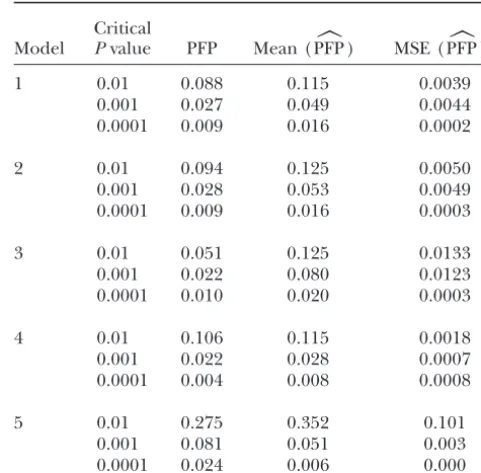
When the method of Mosig et al. (2001) is used to FWER will not guarantee control of the accumulation of false-positive results as a proportion of all positive results over multiple experiments. Obviously the
exam-obtain pˆ0, PFP
典
␣ is the estimator thatMosiget al.(2001)
referred to as “adjusted FDR.” In the simulation
de-ple has been artificially constructed to emphasize the scribed in a subsequent section, we use this estimator
differences among the error measures. This example involves independent experiments, which means that
to produce estimates of PFP (PFP
典
␣) for varying levelsof␣(Table 2).
the tests in one experiment are independent of tests in another. The tests within any of the experiments,
COMPARISON OF PFP, FWER, FDR, AND pFDR however, are not necessarily independent of each other.
Indeed, these tests must be dependent to obtain the
Benjamini andHochberg(1995) defined FDR as
behavior described in the example. Note that when a
large number of rejections occur, the ratioV/Ris high
FDR⫽E
冢
VR
兩
R⬎0冣
Pr(R⬎0), (15) (50/100). On the other hand, when a small number ofrejections occur, the ratioV/Ris quite low (0/10). Such
where, as defined previously,Vrepresents the number of
a situation can arise in the QTL mapping setting.
Sup-mistakenly rejected null hypotheses andRdenotes the
pose that a QTL for a trait of interest lies on a
chromo-number of rejected null hypotheses.Storey(2002)
de-some for which few markers are available. Suppose that fined the pFDR as
some other chromosomes have a high density of mark-ers. A high density of markers on a chromosome without
pFDR⫽E
冢
VR
兩
R⬎0冣
(16) the QTL translates into a high positive correlationamong tests for which the null hypothesis is true.
Be-and proposed pFDR as more suitable than FDR as a cause dense markers are positively correlated, a
false-measure of false discoveries because it more closely positive result at any one of these markers is likely to
matches the type of error control that is desirable in be accompanied by many other false-positive results at
practice. Both FDR and pFDR seem to be gaining in neighboring markers. With few markers on the
chromo-popularity as error measures for multiple-testing prob- some containing the QTL, there can never be a large
lems involving hundreds or thousands of tests. This is number of true positive results. Thus a large number
especially the case in the analysis of microarray data of rejections will occur only when there are a large
where thousands of tests are typical. Familywise error number of false positives. It is in such situations that we
rate [FWER ⫽ Pr(V⬎ 0)] traditionally has been the
will see substantial differences between PFP and the most popular error measure for general multiple-testing
other error measures. Such a scenario is created in problems.
model 5 of our simulation study described later in this We have previously shown that control of PFP across
article. multiple experiments will lead to control of the
propor-Although the example of this section and model 5 of tion of false-positive results among all positive results in
our simulation show that the error measures can differ the long run. We now show by a hypothetical example
substantially, there are many similarities among FDR, that the other error measures (FDR, pFDR, and FWER)
pFDR, and PFP.Storey (2002) has shown that when
do not necessarily share this property.
the tests are identically and independently distributed Suppose that for each experiment in a series of
inde-pFDR⫽ PER;i.e., the level pFDR for a set ofktests is
pendent and identical experimentsV/Ris 50/100 with
equal to the level of PER for a randomly chosen test. probability 0.1, 0/10 with probability 0.5, and 0/0 with
Storey(2003) has shown that pFDR⫽PFP when the
probability 0.4. Then
tests are independent (Corollary 1 inStorey2003) and
that pFDR and FDR will be approximately equivalent
PFP⫽ 50(0.1)
100(0.1)⫹ 10(0.5)⫽
1
3, to PER (and thus PFP) as the number of tests in a family
grows large as long as the test statistics corresponding to which is the proportion of false positives among all
the family of tests satisfy a “weak dependence” condition positive results that will accrue in the long run over
(Theorem 4 inStorey2003). We have shown that the
repeated experimentation. On the other hand, the
val-equality between PFP and PER holds in general regard-ues of FWER, pFDR, and FDR are
less of the dependence structure among the test statistics or the number of tests conducted. A probability
inter-FWER⫽ 1
10, pFDR⫽
冢
50
100
冣冢
0.1
0.1⫹0.5
冣
pretation of pFDR that holds even when tests are notindependent or identically distributed is given below.
⫽ 1
12, FDR⫽
冢
1
12
冣
(0.6)⫽1
20. Let Adenote the event, “a positive result, randomly
selected from all positive results, is a false positive.” We have
Pr(A|R⬎0)⫽兺
k
r⫽1兺 r
v⫽0
Pr(A,V⫽v,R⫽r|R⬎0) QTL model 1:This model had 10 chromosomes with
one QTL at the center of the chromosome; the 10 QTL were of equal effect, so that each accounted for 10% ⫽兺k
r⫽1兺 r
v⫽0
Pr(A|V⫽v,R⫽r,R⬎0)Pr(V⫽v,R⫽r|R⬎0)
of the genetic variance. The remaining 20 chromosomes had no QTL. The simulated trait was completely additive ⫽兺k
r⫽1兺 r
v⫽0 v
rPr(V⫽v,R⫽r|R⬎0) with a heritability of 0.25 in the F2 generation. The
residuals were normally distributed. Each chromosome ⫽E
冢
VR|R⬎0
冣
⫽pFDR. was 100 cM long and had 21 equally spaced markers.QTL model 2:This model was obtained from model
Thus, even when tests are not independent nor identi- 1 by moving the QTL from the center to the left by 25
cally distributed, conditional on an experiment having cM for each of the 10 chromosomes with a QTL.
one or more positive test results, pFDR is equal to the QTL model 3:This model was obtained from model
probability that a randomly chosen test from among 1 by increasing the number of chromosomes with a
these positive results is a false positive. single QTL at the center from 10 to 20 and by decreasing
It is easiest to understand the somewhat subtle differ- the number of chromosomes with no QTL from 20 to
ence between this interpretation of pFDR and the inter- 10. As this model contains 20 QTL of the same effect,
pretation of PFP as PER by considering the example each accounted for 5% of the additive genetic variance.
presented in this section. In the example pFDR is deter- QTL model 4:This model was obtained from model
mined as follows. Of the experiments with at least one 1 by decreasing the number of chromosomes with a
positive result, about five-sixths of the experiments will single QTL at the center from 10 to 5 and by increasing
have 0 as the probability that a randomly selected posi- the number of chromosomes with no QTL from 20 to
tive result will be a false positive while the other one- 25. As this model contained five QTL of the same size,
sixth will have probability 0.5 that a randomly selected each accounted for 20% of the additive genetic variance.
positive result is a false positive. Thus pFDR is (5/6) · QTL model 5: This model with only two
chromo-0⫹(1/6)(0.5)⫽1/12, which is exactly the probability somes was constructed to illustrate that PFP can give
that a randomly selected positive result will be a false quite different results from pFDR and FDR. The first
positive, given that the experiment resulted in at least chromosome was 100 cM long with one QTL at the
one positive result. Note that this calculation in no way center and 11 equally spaced markers. The second
chro-accounts for the fact that there are many more positive mosome also was 100 cM long with no QTL and 101
results in the less likely experimental outcome [Pr(V/ equally spaced markers. The heritability for the trait
R⫽ 50/100)⫽ 0.1] than in the more likely outcome was 0.025.
[Pr(V/R⫽ 0/10) ⫽ 0.5]. On the other hand, PFP ⫽ The scan for QTL was based on testing each marker
PER is the probability that a randomly selected result for linkage to QTL by at-test for comparing the means
is a false positive, given that it is positive. By conditioning for the trait between the two marker genotype classes
on the event that the randomly selected result is positive (Solleret al.1976). The null hypothesis of no linkage
rather than on the event that the experiment contains to a QTL was rejected if the P value for the test was
at least one positive, PFP accounts for differences in the lower than the critical CWER. For each experiment,
number of positive results across experimental out- the numbers of positive (R) and false-positive (V) test
comes because randomly selected events are more likely results were counted given the critical CWER values of
to be positive in experiments with many positive results. 0.01, 0.001, and 0.0001. For each model, 50,000
replica-In contrast to pFDR, experimental outcomes V/R are tions of the experiment were used to obtain empirical
weighted by both their probability of occurrence and values for PFP, pFDR, FDR, and FWER, which in this
the number of rejectionsR. For our hypothetical exam- context is called the GWER (Lander and Kruglyak
ple, we can write PFP as a weighted average of theV/R 1995). The empirical PFP was obtained asV/R,Vand
ratios as R being the mean values of Vand R over the 50,000
replications of the experiment; empirical pFDR was
ob-PFP⫽(0.5)(10)(0/10)⫹ (0.1)(100)(10/100)
(0.5)(10)⫹ (0.1)(100) ⫽
1
3. tained as the mean value of the ratioV/Rover all
experi-ments withR⬎0; empirical FDR was obtained as
empiri-cal pFDR times the proportion of experiments withR⬎
0; and empirical GWER was obtained as the proportion
A SIMULATION STUDY
of experiments withV⬎0. The results for these
empiri-cal values are given in Table 1. A QTL scan with 500 backcross offspring from inbred
lines was simulated. The simulation was used to compare Table 1 shows that PFP, pFDR, and FDR were
practi-cally identical to each other for model 1 through model PFP with FWER, FDR, and pFDR and to illustrate how
the estimated PFP levels compare to true PFP levels. 4, while GWER was very different from these. For these
four models, using a P-value threshold of 0.001 was
The simulation was repeated for five simple genetic
TABLE 2 TABLE 1
Empirical values of PFP, pFDR, FDR, and GWER from Empirical values of PFP, mean values of PFP estimates, and their mean squared errors from 50,000 replicates 50,000 replicates of a simulated backcross
experiment for models 1–5 of a simulated backcross experiment for models 1–5
Critical Critical
Model CWER PFP pFDR FDR GWER Model Pvalue PFP Mean (PFP
典
) MSE (PFP典
)1 0.01 0.088 0.090 0.090 0.825 1 0.01 0.088 0.115 0.0039
0.001 0.027 0.031 0.031 0.194 0.001 0.027 0.049 0.0044
0.0001 0.009 0.012 0.010 0.025 0.0001 0.009 0.016 0.0002
2 0.01 0.094 0.095 0.095 0.824 2 0.01 0.094 0.125 0.0050
0.001 0.028 0.032 0.031 0.192 0.001 0.028 0.053 0.0049
0.0001 0.009 0.012 0.010 0.025 0.0001 0.009 0.016 0.0003
3 0.01 0.051 0.053 0.053 0.581 3 0.01 0.051 0.125 0.0133
0.001 0.022 0.026 0.026 0.104 0.001 0.022 0.080 0.0123
0.0001 0.010 0.013 0.008 0.012 0.0001 0.010 0.020 0.0003
4 0.01 0.106 0.105 0.105 0.889 4 0.01 0.106 0.115 0.0018
0.001 0.022 0.023 0.023 0.237 0.001 0.022 0.028 0.0007
0.0001 0.004 0.005 0.005 0.030 0.0001 0.004 0.008 0.0008
5 0.01 0.275 0.107 0.079 0.111 5 0.01 0.275 0.352 0.101
0.001 0.081 0.030 0.012 0.015 0.001 0.081 0.051 0.003
0.0001 0.024 0.008 0.002 0.002 0.0001 0.024 0.006 0.000
0.05, while with this threshold GWER is well above 0.05.
The results for model 5 show that PFP can be quite from the set ofktests is equivalent to controlling the
different from pFDR and FDR and that pFDR can be PFP defined over allktests. These results hold for any
different from FDR. dependence structure among thektests in an
experi-ment.
When tests are identically and independently
distrib-DISCUSSION uted, pFDR⫽PFP, and thus, in this situation,
control-ling PER for a randomly chosen test is equivalent to In linkage analysis, significance testing has not been
controlling pFDR (Storey 2002). A probability
inter-based on controlling the type I error rate, but on
con-pretation of pFDR that holds even when tests are not trolling the PER, which is the conditional probability
independent nor identically distributed given here is:
of a false-positive result given a positive test result (
Mor-if an experiment with level␥for pFDR has one or more
ton 1955; Ott 1991). For QTL scans, which involve
positive test results,␥is the conditional probability that
multiple tests of linkage, Southey and Fernando
a randomly sampled result from these positive results (1998) proposed PFP as a natural extension of PER,
is a false positive. which was defined for a single test. In this article we
Thus in multiple-test experiments, controlling PFP provided the mathematical justification for this
pro-will result in controlling the proportion of false-positive posal.
results in the accumulated positive test results over many Briefly, the justification is as follows. If the level of
experiments, while controlling pFDR will result in
con-PER for a test is␥, then as the number of independent
trolling the expected proportion of false positives in the tests increases, the proportion of false positives in the
positive test results in each experiment. When tests are
accumulated positive results converges to␥. We have
independently and identically distributed, pFDR⫽PFP,
shown here that if the level of PFP in a multiple test
and, thus, false positives will be controlled to the same
experiment is␥, then as the number of such
indepen-level in each experiment and in the accumulated test dent experiments increases, the proportion of false
posi-results over many experiments. The simulation posi-results tives in the accumulated positive results also converges
for models 1–4 show that even when tests are highly
to␥. Alternatively, we have shown here that when the
dependent, pFDR and PFP can give very similar results.
numberkof tests is 1, controlling PER is equivalent to
For tests that are identically distributed but dependent,
controlling PFP. Further, whenk⬎ 1, we showed that
Elston, R. C., 1997 1996 William Allan award address: algorithms
will converge to PER ⫽ PFP as the number of tests
and inferences: the challenges of multifactorial diseases. Am. J.
increases. As demonstrated by the results for model 5, Hum. Genet.60:225–262.
Elston, R. C., and K.Lange, 1975 The prior probability of
autoso-however, it is clear that in some situations controlling PFP
mal linkage. Ann. Hum. Genet.38:341–350.
is not equivalent to controlling pFDR or FDR.
Genovese, C., and L.Wasserman, 2002 Operator characteristics
Like pFDR, PFP⫽1 if all the null hypotheses tested and extensions of the false discovery rate procedure. J. R. Stat.
Soc. Ser. B64:499–517.
are true. Thus neither pFDR nor PFP can be controlled
Lander, E., and L.Kruglyak, 1995 Genetic dissection of complex
in the same sense that FDR can be controlled (
Benja-traits: guidelines for interpreting and reporting linkage results.
mini and Hochberg 1995). Nonetheless, we believe Nat. Genet.11:241–247.
Morton, N., 1955 Sequential tests for the detection of linkage. Am.
the more direct interpretations of pFDR and PFP make
J. Hum. Genet.7:277–318.
these error measures worth considering. We have
illus-Mosig, M., E.Lipkin, G.Khutoreskaya, E.Tchourzyna, M.Soller
trated the connection between the PER and PFP and et al., 2001 A whole genome scan for QTL affecting milk protein
percentage in Israel-Holstein cattle by means of selective milk
have shown that, unlike FDR and pFDR, PFP is free of
pooling in a daughter design, using an adjusted false discovery
the correlation structure among the tests.Storeyand
rate criterion. Genetics157:1683–1698.
Tibshirani(2001) propose a method for approximat- Nettleton, D., and J.Hwang, 2003 Estimating the number of false
null hypotheses when conducting many tests. Preprint Series
ing FDR and pFDR under general dependence
struc-2003-09, Technical Report, Department of Statistics, Iowa State
tures. Using their method requires the ability to draw
University, Ames, IA.
samples from an approximation to the joint distribution Ott, J., 1991 Analysis of Human Genetic Linkage. Johns Hopkins
Uni-versity Press, Baltimore.
of the test statistics when all null hypotheses are true.
Risch, N., 1991 A note on multiple testing procedures in linkage
This is not a trivial computing exercise and may be very
analysis. Am. J. Hum. Genet.48:1058–1064.
difficult to accomplish in some situations. In contrast, Rohatgi, V. K., 1976 An Introduction to Probability Theory and
Mathe-matical Statistics. Wiley, New York.
the approach to estimate PFP that we have presented
Schweder, T., and E.Spjotvoll, 1982 Plots ofp-values to evaluate
here requires only the P values corresponding to the
many tests simultaneously. Biometrika69:493–502.
tests of interest. Such P values can be obtained with- Soller, M., T.Brodyand A.Genizi, 1976 On the power of
experi-mental designs for the detection of linkage between marker loci
out simulation in situations where the approximate
mar-and quantitative loci in crosses between inbred lines. Theor.
ginal distributions of the test statistics are known. Appl. Genet.47:35–39.
In this article we used the method proposed byMosig Southey, B. R., and R. L.Fernando, 1998 Controlling the
propor-tion of false positives among significant results in QTL detecpropor-tion.
et al. (2001) to estimate p0 and to demonstrate the
Proceedings of the 6th World Congress on Genetics Applied to
estimation of PFP (Table 2). In most of the cases our Livestock Production, Armidale, Australia, Vol. 26, pp. 221–224.
estimates of PFP were conservative. In only two cases Storey, J. D., 2002 A direct approach to false discovery rates. J. R.
Stat. Soc. Ser. B64:479–498.
with very low heritability and one QTL was the mean
Storey, J. D., 2003 The positive false discovery rate: Bayesian
inter-of the estimated PFP levels lower than the empirical pretation and the Q-value. Ann. Stat.31(6): 2013–2035.
value. Even in this case, when estimated PFP wasⵑ0.05, Storey, J. D., and R.Tibshirani, 2001 Estimating false discovery
rates under dependence, with applications to DNA microarrays.
the empirical PFP was only slightly higher. Research in
Technical Report 2001–28, Department of Statistics, Stanford
methods for estimatingp0is ongoing, so we believe the University, Stanford, CA.
Weller, J. I., 2000 Using the false discovery rate approach in the
estimates of PFP illustrated here can be improved by
genetic dissection of complex traits: a response to Zaykinet al.
using improved estimates ofp0. It is also worth noting Genetics154:1919.
that in models 1–4, where the number of QTL ranged
Communicating editor: J. B.Walsh
from 5 through 20, using a critical CWER of 0.001 was
sufficient to control PFP⬍0.05.
APPENDIX
The authors thank two anonymous reviewers for useful comments. R. Fernando acknowledges support from the National Research
Initia-Proof of Property1. LetVidenote the number of
rejec-tive Competirejec-tive Grants Program of the U.S. Department of
Agricul-tions of a true null hypothesis in the ith experiment,
ture, Award 2002-35205-11546; D. Nettleton acknowledges support
from the National Research Initiative Competitive Grants Program and let Ri denote the number of rejections of a null
of the U.S. Department of Agriculture, Award 1998-35205-10390; M. hypothesis in the ith experiment. If we have E(V
i)/
Soller acknowledges support from the BovMAS project of the
Euro-E(Ri)⫽ ␥for alli⫽1, . . . ,n, then the PFP across the
pean Union FP5 program and the Cotswold Swine Breeding Company.
set ofnindependent experiments is given by
E
共兺
ni⫽1Vi兲
E
共兺
ni⫽1Ri兲
⫽
兺
ni⫽1E(Vi)兺
n i⫽1E(Ri)⫽
兺
ni⫽1E(Ri)E(Vi)/E(Ri)兺
n i⫽1E(Ri)LITERATURE CITED
Allison, D. B., G. L.Gadbury, M.Heo, J.Fernandez, C.-K.Leeet
al., 2002 A mixture model approach for the analysis of microar- ⫽
兺
n
i⫽1E(Ri)␥
兺
n i⫽1E(Ri)⫽ ␥.
ray gene expression data. Comp. Stat. Data Anal.39:1–20. Benjamini, Y., and Y.Hochberg, 1995 Controlling the false
discov-ery rate: a practical and powerful approach to multiple testing. This proves property 1.
J. R. Stat. Soc. Ser. B57:289–300.
Benjamini, Y., and Y.Hochberg, 2000 On the adaptive control
Proof of Property2. We begin the proof of property 2
of the false discovery rate in multiple testing with independent
Pr(lim
n→∞
兺
n
i⫽1
{Vi⫺E(Vi)}/n⫽0) ⫽1.
兺
ni⫽1Vi
兺
ni⫽1Ri
⫽
兺
ni⫽1{Vi⫺E(Vi)}/n⫹兺
ni⫽1E(Vi)/n兺
ni⫽1{Ri⫺E(Ri)}/n⫹
兺
ni⫽1E(Ri)/n. (A1)
The same basic argument can be used to show that
By Corollary 1 to Theorem 6 in Rohatgi (1976),
兺n
i⫽1{Vi⫺E(Vi)}/nwill converge to 0, in the almost sure
Pr(lim
n→∞
兺
n
i⫽1
{Ri ⫺E(Ri)}/n⫽ 0)⫽1.
sense, as long as兺∞i⫽1Var(Vi)/i2⬍∞. Note thatViⱕki,
wherekidenotes the number of tests in theith
experi-ment. There existsMⱖkifor allibecause the number Therefore, using (A1), we have
of tests for each experiment does not grow without bound. Thus
lim
n→∞
兺
n i⫽1Vi兺
n i⫽1Ri⫽a.s.
lim n→∞
兺
ni⫽1E(Vi)/n
兺
ni⫽1E(Ri)/n
⫽lim
n→∞
E(
兺
n i⫽1Vi)E(
兺
n i⫽1Ri)⫽ ␥,
ViⱕM, which implies Var(Vi)ⱕE(Vi2)ⱕM2for alli.
It follows that 兺∞i⫽1Var(Vi)/i2 is bounded above by
where the last equality follows from property 1 and
M2兺∞
i⫽11/i2, which is finite. Thus Corollary 1 to Theorem