Performance of Composites from 3D Orthogonal Woven Preforms in terms of Architecture and Sample Location during Resin Infusion.

(1)

ABSTRACT

INCE, MEHMET ERDEM. Performance of Composites from 3D Orthogonal Woven Preforms in terms of Architecture and Sample Location during Resin Infusion. (Under the direction of Dr. Abdel-Fattah M. Seyam and Dr. Mansour H. Mohamed).

Woven preforms are different than laminates due to their complex internal structure such as yarn interlacing, yarn spacing, yarn size, yarn cross-sectional shape, etc. that change the architecture greatly. Another distinguished property of woven preforms is “weave repeat” also called “representative unit cell” which reflects the overall properties of the structure. 3D woven preforms are superior to 2D woven laminates due to presence of through-thickness elements (z-yarn components) that suppress delamination and improve interlaminar properties. The geometry and relative amount of z-yarn is critical to manipulate in-plane and out-of-plane performance. The increase in the z-yarn content leads to improvement in the out-of-plane performance of composite at the expense of in-plane properties.

(2)

Broad range of 3D orthogonal woven preforms from glass fibers with different architectures were woven and consolidated by vacuum infusion process (VIP) with different z-yarn interlacing pattern, number of y-yarn layers, and x-yarn spacing to verify the model for filament yarns.

Dry preform thickness and weight of in-plane yarns predicted by the geometric model for filament yarns correlated well with experimental results. Z-yarn weight of dry preform was 24.3% overestimated by the model due to shortening of z-yarn at cross overs in real preforms due to the flattening of x-yarns caused by the tension of z-yarns. Total FVF of actual dry preform was 0.4% greater than model prediction. However, total FVF of composite was 5.4% overestimated by the model, which is within the experimental error.

(3)

Slight increase from resin inlet to outlet was observed for the tensile properties in x- and y-directions. Due to their higher FVF compared to the composites with other two weaves, composites with twill weaves resulted in better mechanical properties. Increase in x-yarn density caused increase in tensile stress in x-direction, whereas it resulted in reduction in tensile properties in y-direction. Increase in vacuum pressure slightly improved tensile stress in both directions.

Peak tensile stress in y-direction of three layers, 5.48 x-yarns/layer/cm balanced (defined as identical total denier in x- and y-directions/unit sample width) composites manufactured at 100 kPa vacuums was 15.24% greater than peak tensile stress in x-direction due to more uniform placement of y-yarn than x-yarn.

(4)

Performance of Composites from 3D Orthogonal Woven Preforms in terms of Architecture and Sample Location during Resin Infusion

by

Mehmet Erdem Ince

A dissertation submitted to the Graduate Faculty of North Carolina State University

in partial fulfillment of the requirements for the Degree of

Doctor of Philosophy

Fiber and Polymer Science

Raleigh, North Carolina 2013

APPROVED BY:

_______________________________ ______________________________

Dr. Abdel-Fattah Mohamed Seyam Dr. Mansour H. Mohamed

Chair of Advisory Committee Co-chair of Advisory Committee

________________________________ ________________________________

Dr. Mohamed A. Zikry Dr. Xiangvu Zhang

(5)

(6)

BIOGRAPHY

(7)

ACKNOWLEDGEMENTS

I am grateful to Dr. Seyam for his continuous encouragement and guidance throughout the course of my study. I would like to thank Dr. Mohamed for his invaluable suggestions and guidance. Thanks are due to Dr. Meng and Mr. Bracken for providing PPG Industries testing facilities at Shelby, NC that allowed testing the composites’ samples properties. The donation of the E-glass rovings from PPG Industries is appreciated. Great thanks to 3TEX for allowing me to use their winder and to Ashland Inc. for resin donation. I would like to thank my colleagues Tamer Hamouda, Rahul Vallabh, Matthew Laney for their contributions in the formation of the preforms and resin infusion. I am grateful to my dear friend Engin Kapkin

for the training on the use of RhinocerosTM 4.0 software to create 3D orthogonal woven

(8)

LIST OF TABLES

Table 2.1. Maximum fiber volume fractions for different yarn cross sections ... 12

Table 2.2. 3D interlock woven materials ... 33

Table 4.1. Weaves considered for the numerical results ... 70

Table 4.2. Constant input parameters for non-jammed structures with spun yarns ... 70

Table 4.3. Constant input variables for jammed structures with spun yarns ... 72

Table 4.4. Constant input parameters for non-jammed structures with filament yarns ... 89

Table 4.5. Constant input variables for jammed structures with filament yarns ... 91

Table 4.6. Grinding procedure steps ... 94

Table 4.7. Yarn aspect ratios ... 96

Table 4.8. Yarn packing factors ... 97

Table 4.9. Thickness results for 2 layers, plain weave, 4.87 x-yarns/layer/cm structure ... 99

Table 4.10. Constituent yarn weight results for 2 layers, plain weave, 4.87 x-yarns/layer/cm dry preform ... 99

Table 4.11. Constituent yarn FVFs for 2 layers, plain weave, 4.87 x-yarns/layer/cm dry preform and composite ... 99

Table 4.12. Z-yarn angle comparison between model prediction and actual composite ... 99

Table 5.1. Specification of yarns provided by supplier ... 102

Table 5.2. Measured values of x-, y-, and z-yarn linear density ... 102

Table 5.3. Typical liquid resin properties of Derakane® 8084 ... 103

Table 5.4. Typical properties of initiator (NOROX® MEKP-925H) ... 103

Table 5.5. Design of experiment ... 104

Table 5.6. Typical gel times for Derakane® 8084 Resin ... 111

Table 5.7. Flexure test parameters ... 116

Table 5.8. Parameters considered in statistical analysis ... 119

Table 6.1. Mold-filling times of 3 layers dry preforms at 75 kPa vacuums ... 128

(13)

LIST OF FIGURES

Figure 1.1. Dispersed-phase based classification of composites ... 2

Figure 1.2. Matrix-based classification of composites ... 2

Figure 1.3. Classification of 3D fabrics by Khokar ... 6

Figure 1.4. Illustration of conventional 2D weaving principle ... 6

Figure 1.5. Through-thickness angle interlock 3D weave ... 7

Figure 1.6. 3D orthogonal woven fabric ... 8

Figure 1.7. Architecture of 3D orthogonal woven fabric ... 8

Figure 2.1. Unit cell of 3D orthogonal weave ... 11

Figure 2.2. Structures of 3D orthogonal weave in jammed case ... 11

Figure 2.3. Internal unit cell of 3D orthogonal woven preform ... 13

Figure 2.4. Structure of 3D orthogonal woven fabric ... 15

Figure 2.5. Unit cell for 3D orthogonal fabrics ... 16

Figure 2.6. Process window of fiber volume fraction for 3D orthogonal fabric ... 17

Figure 2.7. Schematic of 3D orthogonal weave architecture ... 18

Figure 2.8. 3D orthogonal weave pattern ... 18

Figure 2.9. 3D orthogonal woven structure ... 20

Figure 2.10. Geometric design of 3D orthogonal woven fabric ... 21

Figure 2.11. Different weave patterns for 3D orthogonal woven fabrics ... 22

Figure 2.12. Idealized yarn path of 3D orthogonal woven fabric structure ... 23

Figure 2.13. Lenticular yarn path representation ... 24

Figure 2.14. 3D angle interlock weave architecture ... 24

Figure 2.15. Geometric models of 3WEAVE® fabrics ... 26

Figure 2.16. Effect of changing size of z-yarn ... 27

Figure 2.17. 2D woven structures and corresponding micrographs ... 29

Figure 2.18. 2D fabric architectures ... 30

Figure 2.19. Reflected intensities results ... 30

(14)

Figure 2.21. Weaving process of 3D orthogonal fabric (z-yarn cross sections) ... 32

Figure 2.22. Illustration of 3D interlocking materials ... 33

Figure 2.23. Thick composite systems with different architectures ... 35

Figure 2.24. Multilayer woven structures ... 37

Figure 2.25. Damage area map of impacted specimen ... 38

Figure 2.26. Z-yarn cross section of 3D orthogonal plain woven composite ... 40

Figure 2.27. Effect of fluid pressure on compaction in vacuum infusion ... 44

Figure 2.28. Thickness distribution in vacuum infusion (top) and RTM (bottom) ... 44

Figure 2.29. Schematic of effect of fluid pressure on compaction in vacuum infusion ... 45

Figure 2.30. Evolution of pressure and laminate thickness during vacuum infusion ... 46

Figure 2.31. Thickness variation before, during, and after injection ... 47

Figure 2.32. Predicted pressure profiles for resin flow in plain weave fabric ... 47

Figure 2.33. Predicted and measured thickness profiles for plain weave glass fabric ... 48

Figure 2.34. Final thickness of a vacuum infused continuous strand mat panel ... 49

Figure 2.35. Thickness and fiber volume fraction as a function of location ... 49

Figure 2.36. Variation of fiber volume fraction and fabric thickness in vacuum infusion ... 50

Figure 4.1. 3D orthogonal woven fabric (jammed plain weave) ... 57

Figure 4.2. Generalized non-jammed structure with circular yarn cross section ... 59

Figure 4.3. Generalized jammed structure with circular yarn cross section ... 60

Figure 4.4. Generalized jammed structure with racetrack yarn cross section ... 61

Figure 4.5. Effect of weave factor and z-yarn linear density on constituents and total FVF for non-jammed structure with circular yarn cross section ... 71

Figure 4.6. Effect of weave factor and z-yarn linear density on preform thickness (a), and areal density (b) for non-jammed structures with circular yarns ... 72

Figure 4.7. Effect of weave factor and z-yarn linear density on constituents and total FVF for jammed structures with circular yarn cross section ... 74

(15)

volume fractions for jammed structures with racetrack yarn cross section ... 76

Figure 4.10. Effect of weave factor and z-yarn linear density on preform thickness (a), and areal density of dry preform (b) for jammed structures with racetrack yarns ... 77

Figure 4.11. Generalized non-jammed structure with rectangular yarn cross section ... 80

Figure 4.12. Generalized jammed structure with rectangular yarn cross section ... 82

Figure 4.13. Effect of weave factor and z-yarn linear density on constituents and total FVF for non-jammed structure with rectangular yarns, ... 90

Figure 4.14. Effect of weave factor and z-yarn linear density on preform thickness (a), and areal density (b) for non-jammed structures with rectangular yarns ... 91

Figure 4.15. Effect of weave factor and z-yarn linear density on constituents and total FVF for jammed structures with rectangular yarns ... 92

Figure 4.16. Effect of weave factor and z-yarn linear density on preform thickness (a), and areal density (b) for jammed structures with rectangular yarns ... 93

Figure 4.17. X-yarn cross section of 2 layers, plain weave, 4.87 x-yarns/layer/cm composite ... 94

Figure 4.18. Y-yarn cross sections of 2 layers, plain weave, 4.87 x-yarns/layer/cm composite ... 95

Figure 4.19. Selected spots from x-yarn to determine yarn packing factor ... 96

Figure 5.1. View of the 3D weaving machine (a), multi-insertion of filling yarns (b) ... 104

Figure 5.2. Fabric architecture simulations ... 105

Figure 5.3. Surface images of all 2 layers 3D orthogonal woven dry preforms ... 106

Figure 5.4. Surface images of 4 layers, 5.85 x-yarns/layer/cm dry preforms ... 107

Figure 5.5. Sampling for dry preform characterization ... 107

Figure 5.6. Density kit for volume measurement of analytical specimens ... 108

Figure 5.7. Separation of constituent yarns of dry preform ... 109

Figure 5.8. Z-yarn crimp measurement ... 109

Figure 5.9. Tracing of resin flow fronts at every 3 minutes during infusion ... 112

Figure 5.10. Specimen sampling plan ... 113

(16)

Figure 5.12. Dynatup® drop-tower impact test device ... 117

Figure 6.1. Thickness of 3 layers dry preforms ... 120

Figure 6.2. X-yarn weight of 3 layers dry preforms ... 121

Figure 6.3. Y-yarn weight of 3 layers dry preforms ... 122

Figure 6.4. Z-yarn weight of 3 layers dry preforms ... 123

Figure 6.5. Z-yarn crimp of 3 layers dry preforms ... 123

Figure 6.6. Total weight of 3 layers dry preforms ... 124

Figure 6.7. X-yarn FVF of 3 layers dry preforms ... 125

Figure 6.8. Y-yarn FVF 3 layers dry preforms ... 125

Figure 6.9. Z-yarn FVF of 3 layers dry preforms ... 126

Figure 6.10. Total FVF of 3 layers dry preforms ... 127

Figure 6.11. Tracing of resin flow fronts of 3 layers preforms at 75 kPa vacuum ... 129

Figure 6.12. Tracing of resin flow fronts of 3 layers preforms at 100 kPa vacuums ... 130

Figure 6.13. Thickness profile of 3 layers composites manufactured at 75 kPa vacuums ... 132

Figure 6.14. Thickness profile of 3 layers composites manufactured at 100 kPa vacuums . 133 Figure 6.15. Thickness of 3 layers composites manufactured at 75 kPa vacuums ... 134

Figure 6.16. Thickness of 3 layers composites manufactured at 100 kPa vacuums ... 134

Figure 6.17. Effect of distance from resin inlet on volume-based thickness of composite .. 135

Figure 6.18. Total FVF profile of 3 layers composites manufactured at 75 kPa vacuums ... 138

Figure 6.19. Total FVF profile of 3 layers composites manufactured at 100 kPa vacuums . 139 Figure 6.20. Total FVF of 3 layers composites manufactured at 75 kPa vacuums ... 140

Figure 6.21. Total FVF of 3 layers composites manufactured at 100 kPa vacuums ... 140

Figure 6.22. Effect of distance from resin inlet on composite total FVF ... 141

Figure 6.23. VVF profile of 3 layers composites manufactured at 75 kPa vacuums... 143

Figure 6.24. VVF profile of 3 layers composites manufactured at 100 kPa vacuums... 144

Figure 6.25. VVF of 3 layers composites manufactured at 75 kPa vacuums ... 145

Figure 6.26. VVF of 3 layers composites manufactured at 100 kPa vacuums ... 145

Figure 7.1. Tensile load in x-direction versus strain curve ... 147

(17)

Figure 7.3. Peak tensile stress profile in x-yarn direction of 3 layers composites manufactured

at 75 kPa vacuums ... 150

Figure 7.4. Peak tensile stress profile in x-yarn direction of 3 layers composites manufactured at 100 kPa vacuums ... 151

Figure 7.5. Tensile failure region in x-yarn direction ... 152

Figure 7.6. Tensile failure in x-yarn direction ... 152

Figure 7.7. Effect of distance from resin inlet on tensile stress in x-direction ... 152

Figure 7.8. Effect of number of y-yarn layers on tensile stress in x-direction... 153

Figure 7.9. Constituent yarn FVFs of basket weaves with 5.85 x-yarn density composites 154 Figure 7.10. Effect of weave on tensile stress in x-direction ... 155

Figure 7.11. Constituent yarn FVFs of 3 layers, 5.48 x-yarn density composites ... 155

Figure 7.12. Effect of x-yarn density on tensile stress in x-direction ... 156

Figure 7.13. Constituent yarn FVFs of 3 layers, plain weave composites ... 156

Figure 7.14. Effect of vacuum pressure on tensile stress in x-direction ... 157

Figure 7.15. Tensile specimens in y-yarn direction on the upper-half composite panel ... 158

Figure 7.16. Examples of typical tensile failure in y-direction ... 159

Figure 7.17. Peak tensile stress profile in y-direction of 3 layers composites manufactured at 75 kPa vacuums ... 160

Figure 7.18. Peak tensile stress profile in y-direction of 3 layers composites manufactured at 100 kPa vacuums ... 161

Figure 7.19. Effect of distance (cm) from resin inlet on tensile stress in y-direction ... 162

Figure 7.20. Effect of number of y-yarn layer on tensile stress in y-direction ... 163

Figure 7.21. Effect of weave on tensile stress in y-direction ... 164

Figure 7.22. Effect of x-yarn density on tensile stress in y-direction ... 165

Figure 7.23. Effect of vacuum pressure on tensile stress in y-direction ... 166

Figure 7.24. Tensile stresses of balanced, 3 layers, 5.48 x-yarns/layer/cm composites manufactured at 75 kPa vacuums ... 166

(18)

Figure 7.26. Flexure specimens in x-direction on lower-half composite plate ... 168

Figure 7.27. Profile of peak flexure stress in x-direction of 3 layers composites manufactured at 75 kPa vacuums ... 169

Figure 7.28. Profile of peak flexure stress in x-yarn direction of 3 layers composites manufactured at 100 kPa vacuums ... 170

Figure 7.29. Effect of number of y-yarn layers on flexure stress in x-direction ... 171

Figure 7.30. Effect of weave on flexure stress in x-direction ... 172

Figure 7.31. Effect of x-yarn density on peak flexure stress in x-direction ... 173

Figure 7.32. Effect of vacuum pressure on peak flexure stress in x-direction ... 173

Figure 7.33. Flexure specimens in y-direction on lower-half composite plate ... 174

Figure 7.34. Profile of peak flexure stress in y-yarn direction of 3 layers composites manufactured at 75 kPa ... 175

Figure 7.35. Profile of peak flexure stress in y-yarn direction of 3 layers composites manufactured at 100 kPa vacuums ... 176

Figure 7.36. Effect of distance (cm) from resin inlet on flexure stress in y-direction ... 177

Figure 7.37. Effect of number of y-yarn layers on peak flexure stress in y-direction ... 178

Figure 7.38. Effect of weave on peak flexure stress in y-direction ... 179

Figure 7.39. Effect of x-yarn density on peak flexure stress in y-direction ... 180

Figure 7.40. Effect of vacuum pressure on peak flexure stress in y-direction ... 181

Figure 7.41. Locations of impact specimens on lower-half composite plate ... 181

Figure 7.42. Impact behavior types according to ISO 6603-2 ... 182

Figure 7.43. Load versus deflection diagrams of specimens ... 183

Figure 7.44. Appearances of specimens after impact test ... 184

Figure 7.45. Normalized peak impact load profile of 3 layers composites manufactured at 75 kPa vacuums ... 185

Figure 7.46. Normalized peak impact load profile of 3 layers composites manufactured at 100 kPa vacuums ... 186

(19)

Figure 7.48. Effect of number of y-yarn layers on normalized peak impact load ... 188

Figure 7.49. Effect of weave on normalized peak impact load ... 189

Figure 7.50. Effect of vacuum pressure on normalized peak impact load ... 191

Figure 7.51. Effect of number of y-yarn layers on normalized total penetration energy ... 192

Figure 7.52. Effect of weave on normalized total penetration energy ... 193

Figure 7.53. Effect of x-yarn density on normalized total penetration energy ... 193

(20)

1. INTRODUCTION

Materials are generally grouped into three different categories such as metals, ceramics, and polymers, and each category has its own unique properties. Metals are preferred for strength and toughness, ceramics for strength and transparency, polymers for lightweight and ductility. However, each material group has its drawback, such as metals are heavy, ceramics are brittle, and polymers are low strength.

Today, it is difficult to provide needs for modern technologies (such as aerospace, transportation, and marine) with a single type of material. For example, aerospace industry demands lightweight, strong, stiff, abrasive-corrosive-impact resistant materials. However, it is difficult to produce a product having all these properties by using only one group of materials, because, strong materials are generally heavy and increasing strength of any material results in ductility decrease [1].

The fourth material group to meet the requirement of modern technologies is composites that contain two or more material types without any change in chemical properties of the constituents. The main idea in composites is to combine useful and desired properties of the main materials. A typical example for composite is fiberglass in which short glass fibers are embedded in polymeric matrix. As short glass fibers provide strength and stiffness; polymeric matrix increases ductility and lowers density of the whole structure. Composite phenomena may also be summarized as “moving together” that means the phases of composite respond together to an external (physical, mechanical, environmental) effect [2] [3].

(21)

Figure 1.1. Dispersed-phase based classification of composites

Classification of composites shows that composite science is very broad. The research area of this thesis falls into “Fiber Reinforced Composites” and subcategory of “Continuous (aligned) Fibers”. Composites c also be classified according to matrix type. Figure 1.2 depicts the classification of composites based on type of matrix material.

Figure 1.2. Matrix-based classification of composites

Polymer matrix composites are the most popular one in this classification. They are classified as thermosets and thermoplastics according to type of interaction between polymer molecules. Polymers having intermolecular bonds as strong as covalent bonds in the

Composites

Particle-reinforced

Large-particle

Dispersion-strengthened

Fiber-reinforced

Discontinuous (short)

Aligned Randomly

oriented

Structural

Laminates Sandwich

panels

Composites

Metal matrix composites

Ceramic matrix composites

Polymer matrix composites

(22)

backbone of polymer are called thermoset polymers. These strong bonds are named crosslinks. If bonds between polymer molecules are weak secondary bonding, then this type of polymers are called thermoplastics [3].

The research area of this thesis falls into “Polymer Matrix Composites” and subcategory of “Thermoset Polymers”. Thermoset polymers are generally liquid or easy to melt at room temperature. They may take any shape or be manipulated with reinforcement material in liquid form. In contrast to thermoplastics, which solidify by cooling, thermosets cure (crosslink) and take solid form as result of chemical reaction. Curing process, which is solidification of thermosets, is formation of crosslinks between polymer molecules. Crosslinks between polymer molecules create a unique, interconnected, three-dimensional network structures. Molecular weight of this network structure is dramatically high, which increases melting temperature to a point higher than the degradation temperature. Therefore, thermoset polymers do not melt at high temperature. They char at high temperature. Crosslinking increases not only melting point but also glass transition temperature of polymers.

Main target in the design of “Fiber-reinforced Polymer Matrix Composites” is to get high strength and stiffness by keeping in mind the weight of product. Therefore, for composites, specific strength, which is ratio between strength and density of composite, is an important property. Similarly, for stiffness-based design, specific stiffness that is ratio between stiffness and density of composite is considered. Fiber reinforced polymer matrix composites include low-density fiber and resin; therefore they have high specific-strength and specific-stiffness [1] [3].

1.1. Reinforcement forms (preforms)

(23)

processing and mechanical performance of composites.

Numerous fiber reinforcement forms are available in the market. Fiber itself may be a reinforcement form or it can be converted into different type of sheet forms such as mat and fabric. Textile manufacturing techniques are widely used to produce reinforcement fabric for composite industry [4].

Between 1985 and 1997, woven, braided and knitted textile structures were widely investigated at Langley Research Center under NASA Advanced Composites Technology (ACT) Program. The main aim was to produce main structural parts (such as wing and fuselage) of passenger aircrafts from textile composites. NASA contractors; universities and companies conducted comprehensive research on textile composites especially due to their damage tolerant internal structures as compared to tape laminates (prepregs) [5] [6].

Handling ease is one of the most important advantages of textiles for composites. Due to interlacement between yarns in a textile fabric, it can easily be taken from weaving loom and transported to consolidation area with minimum distortion. Textile technology processes can create preform that has the similar shape of final composite product, therefore; not only part assembly process is eliminated but also more strong joints (bonding) are created compared to other joint types (bolted, adhesive bonded) [7].

3D woven fabrics

The most significant contribution of textile technologies to composite manufacturing is 3D textile structures. Two-dimensional (2D) fiber reinforced composites are very weak against out-of-plane loads, because only weak polymer matrix material resists against out-of-plane loads. Therefore, loads including complex components should not be applied to 2D composites, because separation of layers, which is called delamination, may occur because of plane forces. In order to suppress weakness of 2D composites against complex out-of-plane loads, three-dimensional reinforcement materials were developed [2].

(24)

two-dimensional reinforcements. It is critically important to achieve desired thickness and other dimensions during lay-up process. One of the reasons to eliminate potential dimensional variation of composites is to use direct three-dimensional reinforcements instead of combination of 2D structures. Namely, another advantage of 3D reinforcement is direct preform manufacturing. 3D weaving process forms preform fabrics on volumetric basis, whereas 2D weaving process forms fabrics on areal basis [3] [8].

Fibers placed in thickness direction are called z-yarn, warp weaver, or binder yarn for 3D woven fabrics. More than one layer of fabric is woven at the same time, and z-yarn interlaces warp and weft yarns of different layers during the process. At the end of the weaving process, an integrated 3D woven structure, which has a moderate thickness, is produced. Formability potential of 3D woven fabric is higher than 2D fabrics. 3D fabric has highly porous structure, which decreases resin infusion time compared to stacked 2D woven structures. 3D woven fabrics have also lower or no yarn crimp than 2D woven fabric; therefore, mechanical properties of fibers are almost fully utilized in 3D woven structures. Another advantage of 3D woven structure is being easy to optimize properties for specific directions by strategically placing different fibers in different directions, which is called hybridization [9]. Reinforcement forms having fibers in their thickness direction are stronger against impact and (interlaminar) shear forces between layers. However, placing fibers in thickness direction lowers the amount of fibers available in x-y plane. Therefore, in-plane properties are deteriorated in the presence of through-thickness fibers. If the purpose is just to increase handle ability of preform, then 1% - 2% z-yarn is good enough. In case of great amount of out-of-plane loads, then 33% z-yarn content may be used in through-thickness direction. In final case, a preform having equal load carrying capability in x-, y-, and z-directions is manufactured [2] [3].

Classification of 3D woven fabrics

(25)

Figure 1.3. Classification of 3D fabrics by Khokar

Classification shows that it is possible, using proper weave design techniques, to manufacture 3D woven fabrics using the traditional weaving process (in which one shed is formed at a time; single phase weaving) for manufacturing 2D fabrics.

Figure 1.4 illustrates manufacturing of 2D (a) and 3D fabric (b) on conventional 2D weaving machine. One type of 3D fabrics woven on 2D conventional weaving machine is 3D angle interlock fabric. Weaver or z-yarn in 3D angle interlock fabrics might go through all the thickness of fabric or layer to layer.

Figure 1.4. Illustration of conventional 2D weaving principle (a) 2D fabric, (b) 3D angle interlacing fabric [11]

Figure 1.5 shows a through-thickness angle interlock 3D weave with warp stuffer (y-) yarns 2D weaving

2D fabrics

3D fabrics

- Through-thickness angle interlock - Layer to layer angle interlock

(26)

(blue) seen from its three principles planes and in an isometric view. Warp weaver (z-) yarns are green and weft (x-) yarns are red in the figures.

Figure 1.5. Through-thickness angle interlock 3D weave [11]

(27)

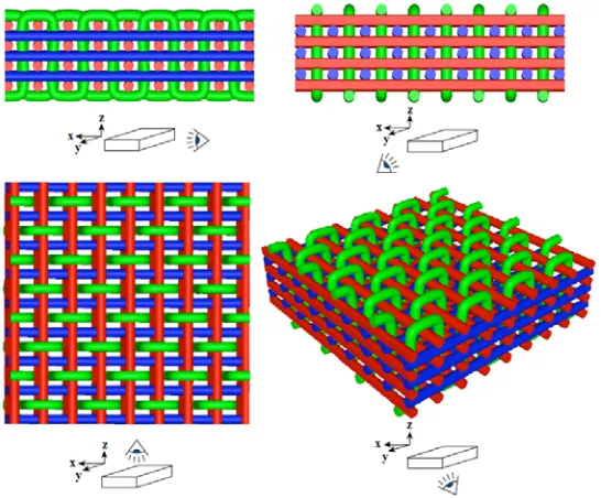
Figure 1.6. 3D orthogonal woven fabric [11]

This new class of fabric is called 3D orthogonal woven fabric and the process to form such fabric was patented by Mohamed and Zhang [14]. The architecture of 3D orthogonal woven fabric consists of three different sets of yarns; warp yarns (y-yarn), weft yarns (x-yarn), and z-yarn. Z-yarn is placed through-thickness of the preform as shown in Figure 1.7.

(28)

(29)

2. LITERATURE REVIEW

The current research deals with fiber-reinforced composites from 3D orthogonal woven structures and thermoset resin. It encompasses geometric modeling of 3D orthogonal preforms from spun as well as continuous filament yarns, effect of fabric architecture on physical and mechanical properties of the final composites, and the effect of sample location from the resin inlet on the physical and mechanical performance. This chapter addresses the relevant previous research in these areas.

2.1. Geometric modeling of 3D woven preforms

(30)

Figure 2.1. Unit cell of 3D orthogonal weave

(note that the unit cell shows only one x-yarn, but maximum total fiber volume fraction calculations in Table 2.1 were based on double x-yarns in unit cell) [15]

(a)

(b)

(c) _(d)

(31)

Table 2.1. Maximum fiber volume fractions for different yarn cross sections Cross-sectional

shape AR*

Maximum fiber volume fractions

(%) (%) (%) (%)**

Circular 1.0 26.18 19.63 13.09 58.90 Elliptical 0.6 26.18 14.73 16.36 57.27 Elliptical 0.3 26.18 9.06 20.14 55.38

Square 1.0 33.33 25.00 16.67 75.00

Rectangular 0.6 33.33 18.75 20.83 72.92

Rectangular 0.3 33.33 11.54 25.64 70.51

Note: Maximum total fiber volume fraction ( ) for elliptical cross-sectional shape with 0.3 aspect ratio was miscalculated as 37.6% in related publication [15]. The model assumes ellipses and rectangles are in

perpendicular (longer dimension of yarn cross section is perpendicular to x-y plane) position. * AR: Aspect ratio (the ratio between short and long dimension of shape)

** Reported in [15]

where

,

in Table 2.1 are the volume fractions of the fiber in x-, y-, and z-yarn

respectively, and is the total fiber volume fraction, calculated from;

2.1.

(32)

Figure 2.3. Internal unit cell of 3D orthogonal woven preform [16]

Overall fiber volume fraction; is defined in equation (2) as:

Total volume of fibers in internal unit cell

The volume of internal unit cell 2.2.

2.3.

2.4.

where

= cross section area sum of fibers in x-yarn (cm2); = cross section area sum of fibers in y-yarn (cm2); = cross section area sum of fibers in z-yarn (cm2); = x-yarn spacing (height of unit cell) (cm);

(33)

= z-yarn spacing (length of unit cell) (cm);

9000 ∗ 100 ∗ 2.5.

N (g/9km) is the linear density of related yarn, and v (g/cm3) is the volumetric density of

fiber composing the yarn. They derived equations to calculate unit cell dimensions for a given set of yarns and constituent yarns’ fiber volume fractions those are lower than the calculated maximum fiber volume fractions given in Table 2.1.

2.6.

2.7.

2.8.

(34)

Figure 2.4. Structure of 3D orthogonal woven fabric [17]

Instead of (x-yarn spacing, also height of internal unit cell in previous model); Gu used

total thickness of the fabric which is expressed as;

2 2.9.

where is the number of y-yarn layers, is the thickness of x-yarn, and is the thickness of z-yarn.

(35)

Ko and Du [19] [20] defined a unit cell for 3D orthogonal fabric, which is shown in Figure 2.5.

Figure 2.5. Unit cell for 3D orthogonal fabrics [19]

They calculated fiber volume fraction based on this unit cell geometry as shown in equation 2.10;

4 2.10.

where , , and are diameters of the yarns in x-, y-, and z-direction, respectively; and

is the yarn packing factor of the yarns. Figure 2.6 shows total fiber volume fraction versus

/ ratios, assuming yarn packing factor of 0.8. The graph was drawn based on three

different / ratios (0.01, 1, and 100). For all / ratios, total fiber volume fraction

firstly decreases with the increase in / ratio, reaches a minimum, and then increases.

(36)

number of layers), and does not include z-yarn cross-over arcs (crowns) on the top and bottom surfaces of the preform. Only circular yarn cross section, which is valid for spun yarns and not valid for filament yarns, was considered.

Figure 2.6. Process window of fiber volume fraction for 3D orthogonal fabric [19]

(37)

They calculated the thickness of individual x- and y-yarn layers in terms of yarn count, yarn spacing, number of layers for each yarn set, and measured composite thickness. However, they did not consider the contribution of z-yarn to overall thickness, yarn cross-sectional shape and its dimensions including yarn packing factor. The experimental results for in-plane properties correlated well with the predicted ones. However, the errors in predicting through-thickness properties were attributed to the difficulty in quantifying the irregularity in through-thickness (z-) yarns.

Figure 2.7. Schematic of 3D orthogonal weave architecture [21]

Cox and Flanagan [6] compiled a NASA contractor report titled “Handbook of Analytical Methods for Textile Composites”. They defined 3D orthogonal woven preform as shown in Figure 2.8.

Figure 2.8. 3D orthogonal weave pattern [6]

(38)

predict fiber volume fraction of yarns in different directions. They showed that in a

composite of thickness with layers of y-yarns alternating with layers of x-yarns, the

volume fractions of y- and x-yarns are simply defined by equations 2.11 and 2.12;

2.11.

and

2.12.

Where is the number of ends (y-yarns) per unit length in the x-yarn direction and is the

number of x-yarns per unit length in y-yarn direction; and are the yields (yield is

defined as yards/liber) of the x-yarn and y-yarn; is the fiber density. The volume fraction

of z-yarn can be written as:

2.13.

Where is the number of z-yarns between successive columns of y-yarns, is the yield of

(39)

Hill and McIlhagger [22] developed a geometric model for 3D orthogonal woven fabrics to calculate total areal weight, and weight percentage of different constituent (x-, y-, and z-) yarns for a given value of the total fiber volume fraction. The model adopted fiber type (volumetric density), yarn count (linear density), yarn spacing, number of layers for each yarn set, limited number of weave patterns for z-yarn, and planned total fiber volume fraction as input parameters. They simplified 3D orthogonal woven structure shown in Figure 2.9 (a) and obtained the simplified geometrical model depicted in Figure 2.9 (b). The model assumed z-yarn path of segmented straight parts and only jammed (maximum construction) case. Their weave interlacing model incorporated different two-harness weaves but did not allow for generalization in terms of weave structure. They did not consider the yarn cross-sectional shape and its dimension including yarn packing factor; therefore, measured cured composite thickness was used in calculations.

(a)

(b)

(40)

Brown and Wu [23] [24] developed a geometric model to predict volume proportions of yarn in x-, y-, and z-directions for 3D orthogonal woven fabric. The model also included overall fiber volume fraction and preform areal density calculation. The length of the unit cell is fixed to 1 cm as shown in Figure 2.10 (b). Similar to the work by Hill and McIlhagger [22], their weave structure model is based on connected straight segments of the z-yarn path. They considered different weave structures as shown in Figure 2.11; however, their model is restricted to two-harness weaves of equal float length for a given weave; therefore, it is not a generalized model. They considered different yarn cross-sectional shapes (circular, elliptical, rectangular) and considered rectangular and hexagonal fiber packing. They also took into account the contribution of z-yarn to overall thickness. Brown and Wu used the constituent material properties of Cox and Dadkhah’s study [21] to validate their model. Their predicted overall fiber volume fraction and thickness from the geometric modeling matched the measurements of Cox and Dadkhah very well. In another experiment, they achieved well correlation between predicted and measured thicknesses.

(a)

(b)

(41)

(a)

(b)

Figure 2.11. Different weave patterns for 3D orthogonal woven fabrics [23]

Brown and Wu [25] used their geometric model to predict stiffness and Poisson’s ratio. They compared their study with the theoretical and experimental results of Cox and Dadkhah [21]. The results showed that the mechanical properties predicted by their model are more close to experimental results than Cox and Dadkhah’s theoretical results. However, there are still discrepancies between their predicted mechanical properties and experimental results. Brown and Wu also indicated the deficiency of their model is related to the unrealistic geometry in which z-yarns were assumed as connected parts of straight segments.

(42)

assumption that z-yarns are formed from connected straight segments for jammed

construction with all yarn systems orthogonal as shown in Figure 2.12.

Figure 2.12. Idealized yarn path of 3D orthogonal woven fabric structure (note that unbounded y-yarn layers on the top and bottom surfaces of the preform) [26]

(43)

Figure 2.13. Lenticular yarn path representation [27]

Buchanan et al. [28] developed and experimentally validated a geometric model for a specific 3D angle interlock woven fabric structure in which the z-yarn forms staircase path. Figure 2.14 depicts the adopted weave architecture in their model study. The model considered the weave repeat and its dimensions. Ellipsoidal cross-sectional shape was adopted. The error between the calculated and experimental results (length and fiber volume fraction) for z-yarn (binder tow) was attributed to assumption of the staircase shape of the z-yarn. The model was also not generalized to include all possible weave patterns of z-yarn.

(a)

(b)

(44)

Byun and Chou [29] developed a model to predict fiber volume fraction and elastic constants of three-dimensional angle-interlock fabric composites. They investigated the architecture by identifying the structural and geometric parameters. The structural parameters were total number of weft threads in the preform and the number of weft threads interlocked by warp threads in the thickness directions. A lenticular geometry was assumed for warp and weft threads cross sections in order to represent thread flattening. They determined elastic constants by using the averaging method and tensor transformation to examine the effects of various structural and geometrical parameters on the elastic properties of the composites. They concluded cross-sectional shape of warp/weft threads and the distance between warp threads in the weft direction of the preform are the key parameters that affect the elastic properties of 3D angle interlock woven composites. They stated that as warp threads interlock more layers in the thickness direction, the thread volume fraction increases and thus improve the composite modulus. The model developed by Byun and Chou is only valid for 3D angle-interlock preform and is not generalized for other weaves.

(45)

Figure 2.15. Geometric models of 3WEAVE® fabrics

[with 12K warp, 12K weft and different size z-yarns: (a) 12K, (b) 6K, (c) 3K, (d) 1K, and (e) 0.1K] [30]

(46)

(a) (b)

(c) (d)

Figure 2.16. Effect of changing size of z-yarn

[Theoretically predicted variations of z-yarn volume content (a), total volume content of resin pockets (b), total fiber volume fraction in a carbon fiber composite (c) and its elastic

(47)

2.2. Effect of fabric architecture on composite formation and performance

Pearce et al. [31] investigated the effects of preform fabric architecture on the processing (composite manufacturing) performance and ILSS (Interlaminar Shear Strength) of fiber reinforced composites produced by resin transfer molding. They used 2D layered woven fabrics with different weave architectures such as; 2x2 twill, 5-harness satin, and 5-harness satin with flow enhanced tow woven at intervals. Figure 2.17 shows the schematics of the weaves and the micrographs of the final composites. All three fabrics had the same areal

density (290 g/m2), and were woven from the same batch of fiber. The permeability ranking

(48)

2x2 twill weave _{5-harness satin weave} 5-harness satin weave with flow enhanced tow Figure 2.17. 2D woven structures and corresponding micrographs

[31]

Thomas [32] used ultrasonic imaging to measure the effect of fabric architecture on through-thickness flow rates during impregnation of an epoxy resin film. He alternately combined ten layers of 2D woven carbon fabrics and epoxy films, which are resin film infusion precursors and manufactured laminates by using vacuum bagging technique. The architecture of woven fabrics is shown in Figure 2.18. Ultrasonic C-scan imaging was performed on the laminates

during infusion in a heated water tank (650C) to be able to monitor reflected intensity, which

(49)

that impregnation rates were directly affected by inter-tow spacing and tow nesting, which are characteristics of fabric architecture, and were indirectly affected by areal densities.

Plain weave 2X2 twill weave

4-harness satin weave 4x4 twill weave

Figure 2.18. 2D fabric architectures [32]

(50)

Brandt et al. [33] compared the mechanical performance of 3D orthogonal woven carbon-epoxy composites with 2D laminates and other traditional 3D angle interlock woven composites. They found that the 3D orthogonal weaving process invented by Mohamed and Zhang [14] manufactures preforms, which have superior mechanical properties compared to other conventional preforms. 3D orthogonally woven composites have higher impact energy absorption capacity, and compression after impact properties than 2D laminates and 3D angle interlock woven composites. 3D orthogonal woven reinforcement greatly impeded the delamination such as; compression strength after impact test (at a 6.7 J/mm impact energy level) of 3D orthogonal fabric reinforced composites was 60% higher than the equivalent 2D laminates as shown in Figure 2.20.

Figure 2.20. Compression strength after impact test [33]

Chou et al. [34] investigated the effect of weave architecture on mechanical (tensile and impact) properties of 3D orthogonal structures from carbon fiber in which z-yarns were

introduced by rod replacement method. Figure 2.21 shows axial (00 and 900,) and off-axis

(±450) yarn placement in 3D orthogonal weaving process. Variables in Chou’s 3D specimens

(51)

structures with a traditional 2D composite. Tensile strength results of the 2D composite were higher than the 3D composites. 3D composites showed stepwise fracture, and were more deformable (having high strain to failure) than 2D composites. In drop-weight impact tests, 3D structures performed better as compared to 2D structures in terms of maximum load, crack initiation, and propagation energies, which were attributed to presence of z-yarn and off-axis yarns in 3D structures. Bogdanovich and Mohamed [30] indicated 3D orthogonal woven composites produced by 3D weaving machine show better or comparable tensile properties to equivalent 2D laminates that shows the advantages of the 3D weaving technique over rod replacement technique in terms of tensile properties.

axial yarn placement off-axis yarn placement

Figure 2.21. Weaving process of 3D orthogonal fabric (z-yarn cross sections) [34]

(52)

Figure 2.22. Illustration of 3D interlocking materials

(note that the other set of z-yarns of 3D orthogonal preform is not shown) [35]

Table 2.2. 3D interlock woven materials

Name Description Warp tow Weft tow Weaver (binder) tow

OS-1 Through-thickness orthogonal

interlock

24 K (59%) 12 K (33%) 6 K (7.4%)

OS-2 12 K (58%) 6 K (37%) 3 K (6.1%)

TS-1 Through-thickness angle

interlock

24 K (57%) 12 K (33%) 6 K (9.8%)

TS-2 12 K (56%) 6 K (38%) 3 K (5.8%)

LS-1

Layer-to-layer interlock 24 K (58%) 12 K (34%) 6 K (6.8%)

LS-2 12 K (57%) 6 K (36%) 3 K (5.9%)

[35]

(53)

three different impact energy levels were used to get a given indent depth for each level, such as; “Barely Visible Impact Damage Level (20.9 J.)”, “Mean Impact Energy Level (53 J.)”, and “Visible Impact Energy Level (85 J.)”. For each 3D weave fabric class in itself, only the effect of tow size on impact response was investigated. The fabric architecture for each class in itself was not changed, which is plain weave for orthogonal fabrics.

Portanova’s study concluded that all 3D woven materials demonstrated comparable damage resistance at the low impact energy level (Barely Visible Impact Damage). OS-1 material had the worst resistance of the 3D weaves with 53% more damage area than best performing TS-1 at the severe impact level (85 J). 3D weaves showed better damage tolerance in tension than in compression. At low energy impact level (20.9 J.) the OS-2 retained 90% of its un-impacted strength in tension but only 65% in compression. All weaves showed moderate compression performance after impact. In tension after impact tests, TS2 and OS2 showed the best results. 3D weaves with larger tow sizes typically had less damage area. For damage tolerance, large fiber bundles resulted in an increase in post-impact strength but a reduction in the percentage of strength reduction. Specifically, the OS-2 material had highest strength in compression, while the TS-2 sample had the lowest percentage of compression strength retention.

Baucom and Zikry [36] investigated the effect of reinforcement geometry on the progression of impact damage and ultimate perforation failure performance at quasi-static crosshead speeds (10 - 80 µm/s) for 2D plain-woven laminates, 3D orthogonal woven laminates, and

3D orthogonal woven monolithic composites. They used S2 glass fiber and Derakane® 8084

(54)

and control of relative properties of the in-plane and z-reinforcements can enable the control of crack initiation, propagation and energy absorption for 3D orthogonal woven preforms.

Figure 2.23. Thick composite systems with different architectures

(a) 2D plain-woven laminate, (b) 3D orthogonal woven laminates, and (c) 3D orthogonal woven monolithic composites [36]

(55)

Baucom and Zikry [38] carried out experimental study to gain understanding of the effects of reinforcement geometry on damage progression in woven composites under repeated drop-weight impact loading conditions. Specimens were 2D plain-woven laminate, 3D orthogonal woven structure, and biaxial reinforced warp knit. The energy level was 18 J (at impact velocity of 2 m/s). 3D composites showed greatest resistance to penetration and absorbed more total energy than the other structures. This unique energy absorption and damage spreading capability was attributed to the presence of through-thickness z-yarn. They stated that straining and fracture of z-yarns acted as additional means of energy absorption. 3D composites spread the energy over wider area, which was attributed to in-plane straight warp and weft yarn placement as compared to greatly undulated yarn placement in 2D woven laminate.

Baucom et al. [39] compared impact performance of 2D woven laminates and 3D orthogonal woven composites. They performed repeated drop weight impact test over specimens at an energy level of 44 J. Damage areas and absorbed (dissipated) energy values of 3D woven composites were greater than 2D woven laminates. Higher damage resistance was attributed to unique fabric architecture of 3D orthogonal woven composites, which incorporate crimped portion of z-yarns in their preform structure. At the conclusion part of the study, they sated that modification of the properties of z-yarn should significantly influence the perforation (puncture) resistance and overall behavior of 3D composite systems.

Desplentere et al. [40] explored the potential of X-ray microcomputer tomography to characterize micro-structural variation of 3D orthogonal woven preforms. They measured yarn thickness, width, and spacing through X-ray micro CT images, and compared them with

the results obtained from surface and cross section images taken by conventional optical

(56)

Padaki et al. [41] investigated the influence of preform interlacement on the low velocity impact behavior of multilayer textile composites. They used structure parameter termed interlacement index “I”, which is defined as number of interlacements in warp and weft divided by the maximum possible contact fields (number of crossover points), to determine structure-impact property relationship. They used high tenacity Nylon-6 filament yarn (96 tex) to manufacture multilayer woven preforms using 4-harness, flexible rapier automatic loom. Woven structures shown in Figure 2.24 were 3D preforms woven on 2D machine. They used hand lay-up technique, unsaturated polyester, and ambient temperature to produce composite structures. In view of impact performance the sequence is 3D orthogonal interlock weave > 3D through-thickness angle interlock weave > 3D layer-to-layer angle interlock weave. They concluded that higher interlacement index of reinforcement results in better impact strength. They also developed impact damage area maps to understand the contribution of different damage mechanisms. Figure 2.25 shows the damage area map adopted to classify different impact failure mechanisms. They showed that increase in interlacement decreases fiber failure area (Figure 2.25) and increases interface failure area. The increase in interface failure area indicates that load (transfer) dissipation capability of composite is increased by interlacement.

(a)

(b) (c)

Figure 2.24. Multilayer woven structures

(57)

Figure 2.25. Damage area map of impacted specimen [41]

King et al. [42] investigated the influence of z-yarn count on fiber volume fraction, yarn crimp, and damage tolerance on 3D orthogonally 5-harness woven composites. They performed dry preform compression testing to predict FVF by using power law relationship between fiber volume fraction and applied pressure. Their FVF prediction from compression tests and FVF values from density buoyancy tests correlated well for 1 bar and 2 bar process pressure values. They stated that a high degree crimp for z-yarn is required to reduce the amount and size of resin rich areas arising from presence of the z-yarn through-thickness direction. It should be mentioned here that crimp of the z-yarn was controlled by the x-yarn spacing and compaction pressure. The higher the x-yarn spacing is (1/x-yarn density), the lower the z-yarn crimp.

(58)

beam shear and bending (flexural) tests to measure interlaminar (transverse) shear properties, and Iosipescu’s shear test to measure in-plane shear properties. Preform heating and increasing consolidation pressure increased bending and shear resistance. He showed that bending and shear properties of 3D orthogonal woven preforms can be improved by adding uniformly covered, thin layer 2D braid to both surfaces of the 3D preform before consolidation. He achieved the highest in-plane shear properties in the case of 45 degree braid angle. He did not measure any impact properties. However, adding 2D braid layer on both surfaces of 3D woven preforms may affect impact behavior, such as crack initiation and propagation profiles are expected to be affected by the presence of off-axis yarns on the surface such as initiated crack may be constricted or spread over a wider area by 2D braid layer.

Gu [17] produced 3D woven composites with different size of z-yarn (3K, 6K, 9K, and 12K) for analytical and mechanical performance tests. As z-yarn size is increased, in-plane fiber volume fractions and correspondingly in-plane mechanical properties decreased. He also did low velocity impact test and mentioned that z-yarn size has negligible effect on impact and post impact performance. However, his impact test device was non-instrumented, and he did not get puncture at the end of impact test by increasing the energy level. In order to evaluate complete energy absorption capability of composite specimen, a full puncture on specimen, and zero force detection on striker are required at the end of the impact test. He also mentioned that more tests such as bending, in-plane shear, and interlaminar shear tests are required to evaluate the effect of z-yarn size on composite mechanical performance.

(59)

than plain weave, which incorporates less interlacing or through-thickness penetration per unit area of preform, should be used in composite production. However, all design options of their study shown in Figure 2.15 consist of plain weave pattern.

Figure 2.26. Z-yarn cross section of 3D orthogonal plain woven composite [30]

The main aim to introduce through-thickness reinforcement is to be able to combat undesirable failure mechanisms in 2D laminates. 3D structures behave similar to 2D laminates in elastic regime, however, in plastic regime where stress is redistributed, and damage accumulation occurs, 3D structures respond quite differently compared to 2D laminates due to presence of through-thickness reinforcement. Therefore, amount and geometry of through-thickness reinforcement element should be thoroughly investigated for designs requiring analysis beyond yield (proportional) limit. Previous studies were limited to jammed plain woven 3D orthogonal preforms. Limiting z-yarn interlacing pattern to plain weave in jammed configuration does not allow investigating fabric architecture potential of 3D orthogonal woven preforms. Infusion performance (measured by resin flow front) of preforms with architectures of different z-yarn interlacing pattern and resultant composites’ mechanical performance beyond yield point in which through-thickness reinforcement plays a great role should be investigated. Additionally, impact damage resistance, post impact tensile and compression strengths, in-plane and interlaminar shear resistance properties

should be investigated for different z-yarn interlacing patterns. The current study addresses

(60)

(61)

2.3. Effect of composite manufacturing technique on thickness variability

It is critically important to select a manufacturing technique, which is suitable to produce a composite product that has required performance characteristics for a specific application. In this study, vacuum infusion process (VIP), which is a subclass of the resin infusion techniques, was used to manufacture composites.

2.3.1. Resin infusion techniques

There are many varieties of resin infusion techniques used by composite industry. Common steps for all resin infusion techniques are; placement of dry preform into mold cavity, closing of mold, injection of liquid resin, and complete wetting of dry preform with liquid resin. After full wetting, resin cures and mold is opened and solid composite structure is taken out [44]. Generally, resin infusion technologies are divided into two main groups namely pressurized injection (resin injected by an injection pump), and vacuum-assisted injection. Resin transfer molding (RTM, pressurized injection)

Resin transfer molding for composites is the same process that is being used in plastic industry for plastic molding. Resin is transferred into the two-sided closed molding by means of pressure. Therefore, it is possible to get smooth surfaces for both faces of composite. Thickness of composites can be adjusted by changing the distance between two rigid surfaces of mold. Injection pressure is generally less than 100 psi or 689 kPa (generally 30 psi or 207 kPa). It is important that mold should be rigid enough not to be distorted by injection pressure. High injection pressure also distorts nature of reinforcement, which is called fiber wash.

(62)

(compression molded) composites. Resin transfer molding is more controllable as compared to VIP, which was described in the following section [46].

Vacuum infusion process (VIP)

Application of pressure in VIP is different than RTM. Pressure is applied into the evacuated mold cavity by atmosphere itself. A vent is opened where last part of dry preform is desired to be wetted. Atmospheric pressure (14.7 psi or 101 kPa) is used for resin flow. There is no need to use two-sided rigid tooling in VIP. One side of tooling is rigid, and other side is flexible vacuum bag. Therefore, tooling cost is lower compared to RTM. VIP is very eligible for large composite parts manufacture. However, surface of composite, which is in contact with vacuum bag, is not smooth. When mold cavity is evacuated, vacuum bag collapses over preform surface and take shape of dry preform surface contour. Therefore, part thickness variation in VIP is higher than RTM [47].

(63)

Figure 2.27. Effect of fluid pressure on compaction in vacuum infusion [48]

Before unclamping of the resin inlet at the beginning of the process, while preform is under vacuum, pressure inside the mold cavity is equal to vacuum pump pressure, and compaction stress on the preform is the difference between atmospheric pressure and vacuum pressure. Once the inlet is unclamped, the resin pressure inside the mold cavity increases which leads to decrease in compaction stress over the preform. Decrease in compaction stress results in change in preform thickness depending on the local resin pressure. Once the mold is filled (resin flow front reaches to outlet), the inlet is clamped, and this section of the process is called post-filling (bleeding). During post-filling, the vacuum pump is still running, and the resin pressure inside the mold cavity both decreases and equilibrates. Therefore, compaction stress over the preform is increased and preform thickness is decreased [50].

Figure 2.28 shows composite thickness (h) is a function of time (t) in vacuum infusion,

whereas thickness is independent from the time for RTM during infusion. Figure 2.29 shows the effect of fluid pressure on preform compaction in vacuum infusion.

(64)

Figure 2.29. Schematic of effect of fluid pressure on compaction in vacuum infusion [51]

(65)

Figure 2.30. Evolution of pressure and laminate thickness during vacuum infusion [50]

Rigas et al. [52] investigated effect of processing conditions on vacuum assisted resin transfer molding process (VARTM). They concluded that thickness variation can be significant, and to some degree, random; in addition, pre-compaction of the preform significantly influences the amount of consolidation pressure needed during infusion. They also stated that dimensional variations due to gradients in the pressure distribution of the vacuum affect permeability (and hence resin flow), as well as dimensional tolerances in manufactured parts. They concluded that VIP is satisfactory for lower fiber volume fraction, thin composites those are used in non-structural/non-ballistic applications, however for thick and high fiber volume applications; the process must be optimized.

(66)

edges. Figure 2.31 shows the thickness variation during the infusion process. The overall decrease in thickness was found rather large, about 10% of the total final thickness.

Figure 2.31. Thickness variation before, during, and after injection (zero-height represents the initial thickness and taken as reference) [53]

Bayldon and Daniel [54] modeled the flow in vacuum infusion process. They also compared their model with experimental study including 2D plain weave fabric (16 plies) and continuous filament random mat (4 plies) and silicone oil as resin. The thickness changes were measured using moiré system. Pressure profile of vacuum infusion of 2D plain weave stack predicted by the model is given in Figure 2.32. Similar pressure profile was also predicted for continuous filament random mat.

(67)

The results show that as flow progresses the pressure gradient at the inlet end becomes very small. They stated that the effect is observed in actual molded components, where the inlet end of the infusion becomes ‘baggy’ and the inlet flow rate becomes very low, even though the flow front is still moving. Figure 2.33 shows the change in thickness profile for the plain weave material. They obtained good thickness profile agreement between model and experiment for saturated region in contrast to unsaturated flow front region, which controls the minimum thickness.

Figure 2.33. Predicted and measured thickness profiles for plain weave glass fabric [54]

(68)

Figure 2.34. Final thickness of a vacuum infused continuous strand mat panel [51]

Correia et al. [51] developed a flow model for vacuum infusion. The model included pressure field prediction and preform compaction. They used the model results to determine distribution of fiber volume fraction and thickness at any point of time including curing time corresponding to final composite. Figure 2.35 shows the model predictions for fiber volume fraction and thickness of six layer stitched bidirectional fabric. They indicated that the thickness data could be used to predict resin consumption. Further, they speculated that the data could be used to predict the local mechanical properties. However, predicting such properties in terms of thickness alone is oversimplified since other parameters such as fiber volume fraction and voids are also varied in terms of sample location.

Figure 2.35. Thickness and fiber volume fraction as a function of location (for stitched biaxial fabric stack with a surface density of 1 kg/m2)

(69)

Hae Park et al. [55] proposed analytical flow model and closed form solutions of vacuum infusion process. They obtained resin pressure profile and fabric compaction stress distribution in closed form solutions. By using fabric compaction stress distribution, they analyzed thickness and fiber volume fraction variation during vacuum infusion process. They used the same input properties of the preform used in Correia et al. [51] work. Fiber volume fraction and thickness profile of Hae Park et al. study are given in Figure 2.36.

Figure 2.36. Variation of fiber volume fraction and fabric thickness in vacuum infusion [55]

Resin flow and absorption of the resin by preform must be evaluated thoroughly in order to produce nonporous, void-free composites by vacuum infusion. Resin flow within preform occurs in two scales such as; macro and micro flow. Macro resin flow that occurs between tows may be visually tracked by using transparent molding. Resin flow between tows is faster than the resin flow within tows between individual fibers. Resin absorption rate is directly affected by inter-tow spacing, which is dictated by fabric architecture. However, areal density indirectly affects the resin infusion rate. Overall, resin infusion rate is affected by fabric architecture, which incorporates macro (inter-tow spacing) and micro porosity (configuration of fibers inside the tow) of fabric, and flow direction [32] [47].

(70)

provides all desired properties to final composite. Therefore, a systematic study to investigate effect of preform architecture and manufacturing technique on analytical and mechanical properties of composites is required for a given preform type and a given composite manufacturing technique [15].

The literature review on the effect of composite manufacturing technique on composite thickness variability showed that the focus of research was on the variation of resin pressure, composite thickness, fiber volume fraction, and there was no research found that address the impact of such variability on the mechanical performance of the final composite in terms of sample location. Additionally, none of the previous research dealt with 3D orthogonal woven composites.