Mathematical Analysis of Sensitive
Parameters on the Dynamical Spread of HIV
S. O. Adewale1, I. A. Olopade2, S. O. Ajao3, I. T. Mohammed4
Associate Professor, Department of Pure and Applied Mathematics, Ladoke Akintola University of Technology
(LAUTECH), P.M.B 4000. Ogbomoso, Oyo State, Nigeria1
Assistant Lecturer, Department of Computer and Mathematics, Elizade University, P.M.B. 002, Ilara-Mokin, Ondo
State, Nigeria2
P.G. Student, Department of Pure and Applied Mathematics, Ladoke Akintola University of Technology (LAUTECH),
P.M.B 4000. Ogbomoso, Oyo State, Nigeria3
Lecturer II, Department of Statistics, Osun State Polytechnic, P.M.B. 301,Iree, Osun State, Nigeria4
ABSTRACT: Sensitivity analysis was performed on a mathematical model of Human Immunodefiency Virus (HIV) to determine the gauge and importance of each parameter to basic reproduction number in the dynamical spread of the disease.
The threshold basic reproduction number
R
0,
which is the average number of secondary infection generated by infected individuals in his or her infectious period was calculated using next generation matrix method, which shows that, the disease dies out whenR
0
1
, and the disease will persist and spread whenR
0
1
.The relative sensitivity analysis was computed for all the parameters in the basic reproduction number, which shows the influence of each parameter in the dynamical spread of the disease. Numerical sensitivity reveals that effective contact rate and progressor rate are the most sensitive parameters in the basic reproduction number. This analysis will help the medical practitioners and policy health makers to know the best control intervention strategies to be adopted in order to reduce dynamical spread of Human Immunodefiency Virus (HIV) in the community.KEYWORDS: HIV, Critical Points, Basic Reproduction Number, Local Stability, Sensitivity I INTRODUCTION
HIV/AIDS is one of the deadliest epidemic diseases the world is still battling with. The onset of the HIV epidemic in sub-Saharan Africa was extremely rapid, with estimated prevalence rate being doubled i.e. each HIV infected person annually infects, directly or indirectly, another (susceptible) individual [26]. Globally there were 36.9 million people living with HIV in 2014 with 2 million people becoming newly infected. Also, 1.2 million people die from AIDS – related illness [22]. In 2015, almost 16 people were receiving antiretroviral therapy [25].
or sharp objects with HIV–infected person, blood transfusion (HIV–Contaminated blood), and mother to child transmission through birth or breast feeding [18].
When a person first infected, he or she may have some symptoms. These symptoms are different from person to person; some may be experiencing cold or flu, fever, headache, sore throat, swollen lymph nodes, fatigue, rash, sores in the mouth especially at the early stage of the disease. However, the only way to tell if your symptoms are from a cold, flu or HIV is to have an HIV tests [21]. One can prevent HIV through the use of condom for sex and by avoiding sharing of needles, sharp objects or other injecting equipments [14]. Antiretroviral (ARV) therapy is the potent treatment for HIV, capable of reducing the virus concentration in the blood to an undetectable level after few weeks of treatment and to sustain the CD4 + T – cell [13, 10]. The use of HAART which is the use of at least 3 antiretroviral drugs has decrease the mortality in HIV – infected patients [15]. When there is no antiviral therapy, the time between HIV – 1 infection and the development of AIDS varies from 5 to 15 years. This depends on the genetic factor or composition of the infected person. There would be rapid multiplication of the virus in the first 2months, after initial infection while the CD4+ T cell population decreases [17]. This makes infected persons become vulnerable to opportunistic infection.
There are many factors that could fuel the spread of HIV. It is important to know these different factors responsible for its transmission and prevalence to determine how best to reduce mortality due to HIV. Thus, in this paper, we examined the most sensitive parameters that play important role in the dynamical spread and control of the disease. We tried to calculate the sensitivity indices of the basic reproduction number that determines whether the disease will die out or become endemic.
II. MATHEMATICAL MODEL FORMULATION
A non linear mathematical model is formulated and analyzed to study the sensitivity of parameters involved in basic reproduction number on the dynamical spread of HIV.
In modeling the dynamics, the population at time t, denoted by N(t), is divided into (5) five compartments of Susceptible (S(t)) individuals, Latently HIV
(
L
H(
t
))
individuals, HIV Undetected(
H
U(
t
))
individuals, HIV Detected(
H
D(
t
))
individuals, Treated HIV(
H
W(
t
))
individuals. So that,)
1
(
)
(
t
S
L
HH
UH
DH
WN
The Susceptible population is increased by the recruitment of individuals into the population at rate
.
the population decrease by natural death rate
. We assumed that susceptible individuals acquire HIV infection, following effective contact with people infected with HIV only (i.e., those in the(
L
H,
UH
U,
dHH
Dand
WH
W)
classes at a rate
H, given by)
2
(
)
(
N
H
H
H
L
H U U dH D W WH H
Where,
H is the effective contact rate for HIV transmission. Then,)
3
(
S
S
dt
dS
H
progression of latent HIV individual to active undetected HIV
H
U (at a rate
H) and also reduced by natural death rate (
) and finally increased by the fraction of Treated HIV at the rate(
)
that moves from treated class to latently HIV compartment. Thus,)
4
(
)
(
1 H H H W
H
H
L
S
dt
dL
The population of undetected infected individuals is increased by the infection of fast progressors (at the rate
(
1
1)
and the development of symptoms by latently individual at the rate(
1
1)
H where
1 is the endogenous reactivation rate. This population is decreased by natural death rate () and disease induced death (at a rate
UH) and further decreased by detection rate (
UH) of HIV undetected infected individuals. Hence)
5
(
)
(
)
1
(
)
1
(
1 H 1 H H UH UH UU
H
L
S
dt
dH
The population of detected infected HIV individual increases by the fraction of latently individuals who develop disease symptoms (at the rate
1
H)
, where
1is the endogenous reactivation rate and the detection of undetected individual at the rate
UH. The population later decreases by treatment rate (
1) for HIV detectedindividual and finally reduces by the natural death rate, induced mortality death rate at
and
UH respectively. Hence we have.)
6
(
)
(
11 H H UH U UH D
D
H
H
L
dt
dH
The population of Treated HIV individuals is increased by those that have received treatment from HIV detected infected individual at the rate (
1) this population reduces by fraction of treated individual that moved back to latently HIV individuals at the rate, (
) since treatment does not completely clears the virus and finally reduced by natural death rate (
).Hence,
)
7
(
)
(
1 D HW W
W
H
H
dt
dH
III. HIV MODEL
)
8
(
)
1
(
5 1
4 1
3 2
1 1 1
W D
W
D U
UH H H D
U H
H U
W H
H H
H
H
K
H
dt
dH
H
K
H
L
dt
dH
H
K
L
K
S
dt
dH
H
L
K
S
dt
dL
S
S
dt
dS
),
(
),
(
),
(
,
)
1
(
),
(
2 1 3 4 1 51 H
K
HK
UH UHK
dHK
HWK
)
9
(
)
(
Where
N
H
H
H
L
H U U dH D W WH H
For this model, it can be shown that the region,
)
10
(
/
:
)
{(
5
S
L
H
H
H
R
N
D
H U U dH D W WFor HIV model only to be epidemiologically meaningful and well posed, we need to prove that all state variables are non-negative for all
t
0
Lemma 1.
The closed set
{(
)
5:
/
S
L
H
H
H
R
N
D
H U U dH D W W }is positively-invariant and attracting with respect to the model (8)
Proof: Consider the biologically-feasible region
D
, defined above. The rate of change of the total population, obtained by adding all equations of the model (8), is given by)
11
(
HW H d UH
N
dt
dN
It follows that
0
dt
dN
whenever
N
. Furthermore,Since
N
dt
dN
, it is clear that
)
(
t
N
if
)
0
(
N
.Therefore, all solutions of the model with initial conditions in
D
remain inD
for allt
0
(i.e., the
-limits sets of the system (8) are contained inD
). Thus,D
is positively-invariant and attracting. In this region, the model can be considered as been epidemiologically and mathematically well posedIII.I Disease Free Equilibrium
For critical points, we set
dt
dS
=
dt
dL
H=
dt
dH
U=
dt
dH
D=
0
(
12
)
dt
dH
WAt disease free equilibrium, it is assumed that there is no infection; Hence (DFE) is given as
( , , , , ) ,0,0,0,0 0
S LH HU HD HW
III.II DERIVATION OF BASIC REPRODUCTION NUMBER (RO) FOR HIV
The Next Generation Matrix (F.V-1) Method
One of fundamental questions of mathematical epidemiology is to find the threshold conditions that determine whether an infectious disease will spread in a population when the disease is introduced into the population [14].
W HW D D H U U UH H H U UH UH H H W H H H H H H H H L K H L K H L K V and S S F ) ( ) ( ) ( ) 1 ( ) ( 0 0 ) 1 ( 1 1 1 1 1 1
After taking partial derivative F and V, we haveF= 0 0 0 0 0 0 0 0 ) 1 ( ) 1 ( ) 1 ( ) 1
( 1 1 1 1
1 1 1 1 W H dH H U H H W H dH H U H H
(13) V= 5 1 4 1 3 2 1 0 0 0 0 0 0 0 K K K K K K UH H (14) Thus,
1
(15)1 1 1 1 ( 1 2 1 1 3 1 1 1 2 5 1 3 5 1 1 2 5 4 1 3 5 4 1 1 1 1 1 5 1 1 4 5 1 1 1 1 1 1 3 1 5 4 3 1 1 2 1 K K K K K K K K K K K K K K K K K K K K K K K K K R UH W W H UH dH H dH U W UH dH UH U H U UH H H UH H T
he threshold quantity
R
H is the basic reproduction number of the normalized model system (8) for HIV infection in a population. It measures the average number of new secondary infections generated by a single infected individual in his or her infectious period in a susceptible population [1].III.III GLOBAL STABILITY OF DISEASE FREE EQUILIBRIUM (HIV)
Here, the global asymptotic stability (GAS) property of the DEF of the HIV model only will be explored.
Theorem3.4: The disease free-equilibrium of the system (8) is globally asymptotically stable whenever
R
H
1
and unstable ifR
H
1
.Proof: It follows that SN*LH HU HDHW at steady state. The proof is based on using the comparison
(16) W D U H W D U H W D U H H H H L Fi H H H L V F dt dH dt dH dt dH dt dL
5 1 4 1 1 1 3 1 2 1 1 1 1 1 10
0
0
)
1
(
)
1
(
)
1
(
)
1
(
=
V)
-(F
K
K
K
K
K
UH H W H dH H U H H W H dH H U H H
According to [6, 31], all eigen values of the matrix (F - V) have negative real parts. Hence, we have
0 ) )( ) 1 )(( ( )) ( )( ) 1 )(( ( ) )( )( ) 1 )(( ( ) )( )( ) 1 )(( ) (( 1 2 1 1 5 2 1 1 5 4 2 1 1 5 4 3 1 1 1 UH H W H UH H dH H H U H U H H K K K K K K K K K K (17)
Thus, from equation (17), the characteristic equation is given by
1 2 2 3 3 4
4
a
a
a
a
Where
1
1
)
1
1
(
)
1
(
3 1 3 1 2 1 1 1 3 4 1 4 1 4 4 1 1 1 1 5 4 3 5 1 5 1 5 5 1 3 3 1 5 4 1 1 4K
K
K
K
K
K
K
K
K
K
K
K
K
K
K
K
K
K
K
a
K
K
K
K
a
H H U H U H H U H dH UH H H dH H H U H H U
1
)1 1 1 1 1 ( 3 1 4 4 3 1 4 2 1 1 4 1 1 3 1 1 1 2 1 5 2 3 5 3 1 5 2 1 1 5 1 3 5 4 1 5 4 1 5 4 4 5 1 5 1 5 1 1 1 1 1 1 1 1 1 2 K K K K K K K K K K K K K K K K K K K K K K K K K K K K K K K K K a H H U H U H H dH H dH UH H UH dH H H U H U H H U H dH UH H H dH H H W UH H W H
)) 1 1 1 1 1 ( ( 3 5 1 1 3 1 1 1 2 1 1 2 5 4 1 2 5 1 1 1 1 1 1 1 4 5 1 1 5 1 1 1 1 3 1 5 4 2 1 3 5 4 1 3 1 1 1 K K K K K K K K K K K K K K K K K K K K K K K K a H dH H W H H UH W H U H UH dH H UH H H U H U H dH UH H W UH UH H H
Applying Routh-Hurwitz criteria of order 4;
.
,
0
,
0
,
0
:
4
a
1a
3a
4and
a
1a
2a
3a
32a
12a
4n
1
,
1
1
1
1
1
(
3 1 5 4 3 1 1 2 1 2 1 1 3 1 1 1 2 5 1 3 5 1 1 2 5 4 1 3 5 4 1 1 1 1 1 5 1 1 4 5 1 1 1 1 1 1
K
K
K
K
K
K
K
K
K
K
K
K
K
K
K
K
K
K
K
K
K
K
K
K
K
H UH UH W W H UH dH H dH U W UH dH UH U H U UH H
Hence, we have established that the disease free equilibrium is globally asymptotically stable whenever
R
H
1
and unstable whenR
H
1
.
III.IV EXISTENCE OF ENDEMIC EQUILIBRIUM (EE)
Where
0*
(
S
**,
L
*H*,
H
U**,
H
D**,
H
W**)
are the endemic equilibrium points. Equation (8) becomes)
5
.
18
(
)
4
.
18
(
)
3
.
18
(
)
1
(
)
2
.
18
(
)
1
.
18
(
5 1 4 1 3 2 1 1 1 W D W D U UH H H D U H H H U W H H H HH
K
H
dt
dH
H
K
H
L
dt
dH
H
K
L
K
S
dt
dH
H
L
K
S
dt
dL
S
S
dt
dS
Solving equation
18
.
1
-18
.
5
at steady state and re-writing in terms of
*H*S
**, we have)
6
.
18
(
* * * * 1 **S
L
HH
)
9
.
18
(
...
...
...
...
...
)
8
.
18
(
...
...
)
7
.
18
(
...
...
)
1
(
* * * * 4 5 * * * * 3 1 * * * * 3 4 * * * * 2 4 * * * * 1 1 * * * * 2 3 * * * * 1 12 3 * * * * 1 ** **S
P
K
S
P
H
S
P
K
S
P
K
S
P
K
H
S
P
K
S
P
K
K
K
S
H
H H W H H UH H H D H H H H U
WhereY
X
P
1 1 UH(
1
1)
1
Y
X
K
K
K
Y X K K K K Y X K
P H UH(1 ) UH (1 ) H 1 1 UH(1 1)
3 2 2 1 4 1 1 1 4 1 3 Y X K K K K Y X K K
P H UH(1 ) UH (1 ) H UH(1 )
. 1 1 1
3 12 2 1 4 1 1 1 4 1 5 1 4 Where
3 5 4 1 12 1 5 4 1 1 1 11
K
K
K
K
K
K
K
K
w
K
X
H
UH
H
3 5 4 1 12 1 5 4 1 1 1 3 5 4 11
K
K
K
K
K
K
K
K
K
K
K
K
K
K
Y
H
UH H
) 10 . 18 ( * * * * * * * * * * N H H HLH U U dH D W W H H
Substituting the expressions in (
33
.
14
–33
.
17
) into (33
.
18
) we have
** 1 ** ** 2 ** ** 3 ** ** 4 ** **
** **
1 2 3 4
(18.11)* * P P P P S S P S P S P S P
S H H H H H U dH W
H
Divide each term in (
18
.
11
) by ** ** SH
1 2 3 4
* * 5
1
P
P
UP
dHP
WP
Where
P
5
P
1
P
2
P
3
P
4
0
So that
A
K
K
K
K
A
K
K
K
K
K
A
K
K
K
A
K
K
A
K
K
K
K
A
K
K
K
K
K
A
A
K
K
K
A
A
K
K
K
K
K
K
K
A
A
K
K
K
K
K
K
K
K
P
UH H UH H UH UH UH H H UH H UH H UH UH UH H UH H UH H 3 4 1 1 2 5 1 2 5 1 1 1 15 1 1 1 1 3 1 1 1 13 14 1 1 2 5 1 2 5 1 1 1 1 5 3 1 1 1 1 5 4 1 2 5 4 1 1 1 1 1 5 4 3 1 5 4 3 1 * * 5)
1
(
)
1
(
)
1
(
)
1
(
)
1
(
)
1
(
)
1
(
)
1
(
)
1
(
)
(
1
where
Q
R
H
5 4 1 5 1 4 5 1 1 1 1 2 1 2 3 4 1 1 3 1 1 1 4 5 2 1 1 4 5 3 1 5 4 3 12
2
)
1
(
2
)
1
(
)
1
(
3
2
K
K
K
K
K
A
K
K
K
K
K
K
AK
K
A
A
K
K
K
A
K
K
K
K
K
A
K
K
K
K
K
K
Q
H UH H UH UH H UH H H
Where
3 5 4 1 12 1 5 4 1 1 11
K
K
K
K
K
K
K
K
K
K
w
A
H
uH H0
1
5 *
*
P
Q
R
H
Whenever
R
H
1
(
19
)
III.V HIV SENSITIVITY ANALYSIS
This analysis will help us to know which of the parameters causes most reduction in
R
oand parameters that have highimpact on
R
o and these should be targeted by intervention strategies in order to have most effective control of the disease. This analysis tells us how crucial and important each parameter is to disease transmission. We compute the normalized forward sensitivity index of the reproduction number with respect to its parameters.Definition: If a variable ‘b’ depends differentiably on a parameter ‘u’, then, the normalized forward sensitivity index of
‘b’ with respect to ‘u’ is denoted by Xb, which is defined as
b
u
u
b
X
b
As we have explicit formula for
R
o, we derive an analytical expression for the sensitive ofR
o as)
20
(
o o R
b
R
u
du
dR
X
o
Sensitivity analysis for each parameter involved in
R
His therefore calculated. The results obtained were tabulated below as follows:Table III.I Values of Numerical Sensitivity of HIV PARAMETERS SENSITIVITY VALUE
1
-0.141060
-0.096178dH
-0.074683UH
-0.789652
-0.223921UH
-0.083820U
0.000401W
-0.000034dH
-0.0000201
0.0906731
0.763369H
1.000000H
Table III.II: Variable and Description VARIABLES DESCRIPTIONS
S Susceptible individuals
H
L
Latent HIV individualD
H
Detected HIV individualU
H
UndetectedHIV individualW
H
Treated HIV individualTable III.III: Parameters and Descriptions PARAMETERS DESCRIPTIONS
Recruitment rate
Natural death rate1
Treatment rate1
Fast progressorH
Progression rateUH
Detection rate
Loss of immunityH
Effective contact ratedH UH
,
Disease induced rateW dH
U
,
,
Modification parameters IV. NUMERICAL SIMULATIONS OF THE MODELIn order to verify the dynamical behavior of the model, the numerical simulations is analyzed by using Runge –Kutta method using the following set of parameter values:
2
.
0
,
0.02
,
1
0
.
2
,
dH
0
.
1
,
UH
0
.
3
,
0
.
7
,
0
.
2
UH
,
U
0
.
001
001
.
0
W
,
dH
0
.
001
,
1
0
.
7
,
H
0
.
1
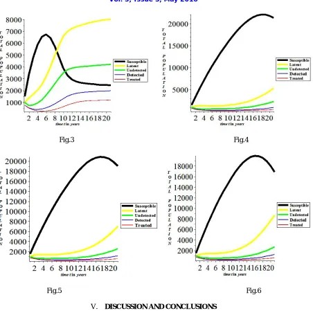
Fig.3 Fig.4
Fig.5 Fig.6
V. DISCUSSION AND CONCLUSIONS
It is observed that effective contact rate in Fig. 1, 2 and 3, reduces the susceptible individuals and increases latently infected individuals, infected undetected individuals and infected detected individuals. It reduces susceptible individuals from 23000 to 2500 due to an increase in effective contact rate from 0.1 to 0.5. In Fig. 4, 5 and 6, the effect of fast progressor is shown. It can be seen that as progressor increases, the susceptible individuals decreases while the latently infected, infected undetected and infected detected individuals increases. It is noted that the fast progressor can be controlled when the immunity of an individual is very strong.
REFERENCES
[1] AIDS info: Fact sheets: HIV prevention, The basics of HIV Prevention. U. S. Department of Health and Human Service (HHS). Available at https://aidsinfo.nih.gov/education-materials/fact-sheets/20/48/the-basics-of HIV-prevention.
[2] S.O. Adewale, C.N. Podder and B. Gumel. Mathematical analysis of a Tuberculosis (TB) transmission model with DOTs. Canadian Applied Mathematics Quarterly. Vol.17,No.1, Spring 2009.
[3] C. Castillo- Chavez and B. Song. Dynamical models of Tuberculosis and their applications. Mathematical Biosciences. Vol.1, pp.361-404, 2004.
[4] Centers for Disease Control and Prevention (CDC): HIV Transmission. Available at www.cdc.gov/hiv/basics/transmission.html. Accessed on 21/01/16
[5] M. B. Feinberg, Changing the natural history of HIV – disease. Lancet. Vol. 348, pp 239 – 246, 2006.
[6] A. Gumel and B. Song. Existence of multiple stable equilibria for a multi – drug resistance model of mycobacterium TB. Mathematics Biosci. and Engineering. 5(3):437-455, 2008.
[7] B.H. Hahn. Tracing the origin of the AIDS pandemic. The PRN Notebook. Vol. 10. No. 3, 2005.
[8] S. Hochmen and K. Kim. The impact of HIV co-infection on cerebral malaria pathogenesis. Journal of Neuroparasitology. Vol. 3. Article ID 235547, 2012.
[9] R.S. Janssen , D.R. Holtgrave R. O. Valdiserri , M. Shepherd., H. D. Gayle and K. M. De cock The serostatus approach to fighting the HIV epidemic: prevention strategies for infected individuals. Am. J. Public Health. Vol. 91, pp. 1019 – 1024, 2001.
[10] G. R. Kaufmann, L. Perrin and G. Pantaleo, CD4+ T – lymphocyte recovery in individuals with advanced HIV – 1 infection receiving potent antiretroviral therapy for 4 years: the Swiss HIV cohort study. Arch. Intern. Med. Vol. 163,pp 2187 – 2195, 2003.
[11] V. Lakshmikantham, S. Leela. and A. A. Martynyuk X Stability analysis of Non-Linear system. Marcel Dekker, Inc; New York and Basel. 1989
[12] P. Lampley, M. Wigley, D. Carr and Y. Collymore, Facing the HIV/AIDS Pandemic. Population Bulletin. Vol. 57, No. 3, 2002.
[13] A. Mocroft, A. N. Phillips and J.Gatell, for the EuroSIDA study Group (2007); Normalization of CD4 counts in patients with HIV-1 infection and maximum virological suppression who are taking combination antiretroviral therapy: an observational cohort study. Lancet. Vol. 370, pp. 407 – 413, 2007.
[14] NHS choices: HIV and AIDS – Prevenvetion. Available at nhs.uk/conditions/hiv/pages/preventionpg.aspx. Accessed on 20/01/16
[15] W. B. Park, H. C. Jang, , S. H. Kim, H. B.Kim, N. J. Kim, M. D . Ohand K. W. Choe Effect of Highly Active Antiretroviral Therapy on early syphilis in HIV – infected patients. Sexually Transmitted Diseases. Vol. 35, No. 3, pp. 304 – 306, 2008
[16] J. Putzel. Institutionalizing an Emergency Response: HIV/AIDS and Governance in Uganda and Senegal. A report submitted to the department for International Development. 2003.
[17] L. Renia and S. M. Potter. Co-infective of malaria with HIV: an immunological perspective. Parasite Immunology.Vol.28, pp 589 – 595, 2006.
[18] L. W. Roeger, Z. Feng and C. Castillo – Chavez. Modeling TB and HIV Co-infections. Mathematical Biosciences and Engineering, Vol. 6, No. 4. pp. 815 – 837, 2009.
[19] O. Sharomi , C. N. Podder, A. B. Gumel, and B. Song. Mathematical analysis of the transmission dynamics of HIV/ TB Co-infection in the presence of treatment. Mathematical Biosciences and Engineering. Vol. 5, No. 1, pp 145 – 174, 2008.
[20] P. Srivastava, , M. Banerjee, and P. Chandra. Dynamical model of in- host HIV infection: With drug therapy and multiviral strains. Journal of Biological Systems, Vol. 20, No. 3. pp 303 – 325, 2012.
[21] U.S Department of Veterans Affairs: HIV/ AIDS: what are the symptoms? Available at www.hiv.va.gov/patient/basics/symptoms.asp. Accessed on 20/01/2016.
[22] UNAIDS: Fact sheet. Available at www.unaids.org/en/resources/campaigns/HowAIDSchangedeverything/factsheet.Accessed on 20/01/2016 [23] P. Van den Driessche and J. Watmough. Reproduction numbers and sub-threshold endemic equilibria for compartmental models of disease
transmission. Mathematical Biosciences. Vol. 180, pp 29 – 48, 2002.
[24] W. Wang. Backward bifurcation of an epidemic model with treatment. Math. Biosci. 201(1-2): 58 – 71, 2006. [25] WHO. HIV /AIDS. Available at www.who.int/hiv/en/. Accessed on 20/01/2016.