On probabilistic analysis of randomization in
hybrid symbolic-numeric algorithms*
Erich Kaltofen, Zhengfeng Yang
Department of Mathematics North Carolina State University Raleigh, North Carolina 27695-8205, USA
kaltofen,[email protected]
http://www.kaltofen.usLihong Zhi
Key Laboratory of Mathematics Mechanization Academy of Mathematics and Systems Science
Beijing 100080, China
[email protected]
http://www.mmrc.iss.ac.cn/~lzhi/ABSTRACT
Algebraic randomization techniques can be applied to hy-brid symbolic-numeric algorithms. Here we consider the problem of interpolating a sparse rational function from noisy values. We develop a new hybrid algorithm based on Zippel’s original sparse polynomial interpolation tech-nique. We show experimentally that our algorithm can han-dle sparse polynomials with large degrees. We also give a (partial) mathematical justification why the Zippel’s alge-braic randomization technique can be used with our ap-proximate data: the randomly generated non-zero values are expected to be bounded away from zero. We show that the random Fourier-like matrices arising in our algorithm, have the desired rank property in the exact case, and appear usable numerically.
Furthermore, we show that Sylvester matrices of poly-nomials with nonidentically distributed random coefficients have large condition numbers. That phenomenon has pre-cluded several algebraic randomization techniques from use in the approximate hybrid setting.
Categories and Subject Descriptors: I.2.1
[Comput-ing Methodologies]: Symbolic and Algebraic Manipulation —Algorithms; G.1.2 [Mathematics of Computing]: Numeri-cal Analysis—Approximation
General Terms:algorithms, theory, experimentation
Keywords: multivariate rational function, interpolation, sparse polynomial, random matrix, structured matrix, con-dition number, probabilistic analysis, symbolic/numeric hy-brid method
∗
This research was supported in part by the National Science Foun-dation of the USA under Grants CCF-0514585 (Kaltofen and Yang) and OISE-0456285 (Kaltofen, Yang and Zhi), and by NKBRPC (2004CB318000) and the Chinese National Natural Science Founda-tion under Grant 10401035 (Zhi).
Permission to make digital or hard copies of all or part of this work for personal or classroom use is granted without fee provided that copies are not made or distributed for profit or commercial advantage and that copies bear this notice and the full citation on the first page. To copy otherwise, to republish, to post on servers or to redistribute to lists, requires prior specific permission and/or a fee.
SNC’07, July 25–27, 2007, London, Ontario, Canada.
Copyright 2007 ACM 978-1-59593-744-5/07/0007 ...$5.00.
1.
RANDOMIZATION IN ALGEBRAIC
AND HYBRID COMPUTATION
Since the discovery of the Zippel-Schwartz lemma [6,38, 43] in 1979, randomization techniques based on introduc-ing elements that have been randomly sampled from a fi-nite subset of the domain of scalars have become ubiqui-tous. Zippel’s original application was to sparse multivariate polynomial interpolation [44,45], Schwartz’s to establishing polynomial identities, and DeMillo’s and Lipton’s to proving programs correct by executing at random inputs.
A classical application is to compute the GCD of many polynomials by computing the GCD of random linear com-binations [21, Theorem 6.2 and Note added in proof]. Im-portant applications are the effective Hilbert irreducibility theorems [13, 20,25] for polynomial factors and precondi-tioning of dense, sparse and black box matrices [2, 27,28, 42]. Randomization is needed in Gao’s polynomial factor-ization algorithm [11] and in solvers for linear systems whose coefficient matrices have small displacement rank [24, Ap-pendix]. There are many more examples for exact symbolic algorithms.
Hybrid symbolic-numeric algorithms permit errors in the input scalars due to floating point round-off or through phys-ical measurement. In order to obtain a non-trivial solution, the algorithms minimally deform those input variables to obtain the desired result, say
1. a solution to an inconsistent system of linear and polyno-mial equations (total least squares: TLS [16], structured TLS: STLS [32, 34], symbolic-numeric elimination [15, 17,33,35]),
2. the GCD of relatively prime polynomials (approximate GCD [4,8,30,36]),
3. a non-trivial factorization of irreducible multivariate poly-nomials with real or complex coefficients (approximate factorization [12,26,37]),
4. a univariate rational function interpolant [19] and a sparse multivariate interpolant (sparse numeric interpolation of polynomials: SNIP [14], sparse numeric interpolation of rational functions: SNIPR [29]).
allows the elimination of singular cases. In the hybrid set-ting, the same randomization can avoid ill-conditioned sub-problems [12,14,26], unstable divisions by elements that are near zero, or areas of divergence or local minima in iterative refinement [30].
In Section2we consider the approximate GCD problem when using random projections of the coefficients. In par-ticular, we investigate the condition number of the Sylvester matrix of random polynomials. Large random dense matri-ces with random entries from a standard Gaussian distri-bution have a small condition number [3], and random per-turbations of the entries of well-conditioned dense matrices remain well-conditioned [39]. Because of the root distribu-tion of random polynomials, the Sylvester matrices of two random polynomials with coefficients from a Gaussian dis-tribution have a similar expected values of their condition numbers. We exploit such well-conditionedness in our new rational function interpolation algorithm. When the coef-ficients are binomially distributed, however, the roots con-centrate on the real axis and the condition numbers of the corresponding Sylvester matrices become very large. The latter phenomenon caused our earlier hybrid SNIPR algo-rithm in [29, Section 6] to fail on large degree inputs.
In Section 4we present our hybrid ZNIPR algorithm for numerically interpolating rational functions from noisy val-ues. We adapt Zippel’s original variable-by-variable sparse polynomial interpolation algorithm in two ways: first, we show how to deploy the algorithm for sparse rational func-tions and give a complete probabilistic analysis (Section4.1) for exact arithmetic. We then use the algorithm in the set-ting where the rational function values are noisy. Our ex-periments show that the method can handle large degree polynomials, unlike our earlier SNIPR method. In Section3 we show that Zippel’s assumptions have a justification in the numerical hybrid setting. As said above, the needed relative primeness assumptions can also be understood. Finally, it may be possible to also give estimates on the condition num-ber of the arising random Fourier-like matrices from recent work in signal processing.
2.
APPROXIMATE GCD OF RANDOM
UNIVARIATE POLYNOMIALS
Let {aj(ω)}∞j=0 denote a sequence of random variables
with respect to the distributionω. Letpd(x) =Pdj=0aj(ω)xj
denote the random univariate polynomial of degreeddefined by the sequence{aj(ω)}. Letα, βandδ be three arbitrary
numbers such that 0≤α < β≤2π, and 0< δ≤1. Con-sider the following subsets of the complex numbers:
B={z∈C:α <argz < β}
C={z∈C: 1−δ≤ |z| ≤1 +δ}.
The following result is stated and proved in [40], see also [1, Theorem 8.1]:
Theorem 2.1 Let the coefficientsaj(ω) of a random
alge-braic polynomialpd(x)be independently and identically
dis-tributed complex-valued random variables, let the expected value
E(max{0,log|aj|})<∞for allj= 0,1, . . . , d,
and letNd(B, ω) andNd(C, ω) denote the expected number
of zeros of the random polynomials that are contained in the
setB andC, respectively. Then
lim
d→∞
Nd(B, ω)
d =
β−α
2π and dlim→∞
Nd(C, ω)
d = 1.
Theorem2.1tells us, as the degree of the polynomial in-creases, the zeros tend to concentrate on the circumference of the unit circle and appear to be uniformly distributed. Moreover, it is also shown in [1, Theorem 8.5], as the num-ber of sample polynomials increase, the sample zeros cluster about the averaged zeros. This implies that the probabil-ity for random polynomials having common roots increases along with the growth of degrees of polynomials. So high de-gree random polynomials always have an approximate GCD within fixed precision deformation [5]. However, we also notice that for random polynomials with independent and normally distributed coefficients, the condition number of the Sylvester matrix generated by the polynomials increases almost linearly in the degrees of polynomials, as is the case for arbitrary dense matrices [3, Theorem 6.1]:
Theorem 2.2 For anm×ncomplex random matrixGm×n
whose elements are independent and identically distributed standard normal random variables, then the expected loga-rithm of the2-norm condition number satisfies:
E(logκ2(Gm×n))<log n
n−m+ 1+ 2.258,
for anyn≥m≥2.
We do not know if the structured condition number for Sylvester matrices of random polynomials with normally distributed coefficients, which is smaller than the condition number, has linear growth.
For the univariate polynomials coming from the ZNIPR algorithm of Section4, the coefficients of these polynomials distributed almost independently and normally, the degrees of polynomials used for Table 1 and 2 are less than 100, so by the arguments above, the roots of these univariate polynomials are well separated and the condition numbers of the Sylvester matrices are relatively small (in the 100’s). If the random polynomials have nonidentical coefficients, then the zeros of these random polynomials are distributed differently from the zeros of random polynomials with Gaus-sian coefficients. For example, as reported in [9, 10], the random polynomial of the form
pd(x) = d
X
j=0
aj(ω)
q`d j
´
xj (1)
with Gaussian coefficients{aj(ω)}dj=0has
√
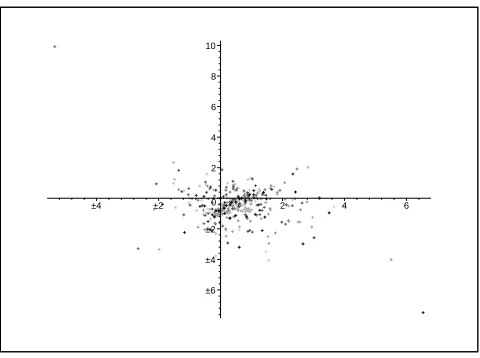
dreal zeros on average, while polynomials with identically distributed co-efficients have fewer than (2 logd+ 14)/πreal roots ford→ ∞[18]. See Figures1and2for the distribution of the zeros of the random polynomials of degrees 20 with coefficients distributed identically and binomially respectively.
Moreover, we observe that the condition numbers of Sylvester matrices generated by the random polynomials with bino-mial coefficients increase exponentially in the degrees of the polynomials. That explains why the condition numbers of the Sylvester matrices come from the SNIPR algorithm are huge even for polynomials with moderate degrees. The ran-dom univariate polynomials obtained by evaluating y ←
–1.5 –1 –0.5 0 0.5 1 1.5
–2 –1 1 2
x
Figure 1: Roots for identically distr. coeff.’s
–6 –4 –2 0 2 4 6 8 10
–4 –2 2 4 6
Figure 2: Roots for binomially distr. coeff.’s
circle, have coefficients distributed binomially. A mathe-matical analysis of the condition number and structured condition number of Sylvester matrices of polynomials with non-identically distributed coefficients, say as in (1), appears open.
3.
A NUMERIC ZIPPEL-SCHWARTZ
LEMMA
In Section4we will employ the randomization as in Zip-pel’s original application, namely to determine if coefficient polynomial is identical zero by computing its value at a ran-dom point. We need to show that for certain ranran-dom points, polynomial values are actually bounded away from zero.
Lemma 3.1 Let 0 6= h(y1, . . . , yr) ∈ Z[i][y1, . . . , yr] and
for all 1≤i≤r let pi = exp(2π i
bi )∈C, with the bi∈ Z≥3
distinct prime numbers. Supposeh(p1, . . . , pr) 6= 0. Then
for random integerssiwith1≤si< bi the expected value
E{|h(ps1
1 , . . . , p
sr r )|} ≥1.
Proof. Let B = b1· · ·br and let ζB = exp(2Bπi). The
cy-clotomic polynomial ΦB(z) of order B is irreducible over
Q(i). Thereforeh(ps1
1 , . . . , psrr) is an automorphic image of h(p1, . . . , pr) inQ(ζB,i) overQ(i) and thus non-zero. We
have for the norm
06= Y
1≤s1<b1
· · · Y
1≤sr<br h(ps1
1 , . . . , p
sr
r )∈Z[i].
Therefore forN= (b1−1)· · ·(br−1) we have by the
arith-metic-geometric mean inequality 1
N
X
|h(ps1
1 , . . . , p
sr r )| ≥ N
qY
|h(ps1
1 , . . . , p
sr
r )| ≥1.2
By the Schwartz-Zippel lemma we can achieve the premise
h(p1, . . . , pr) = 0 with high probability. Since all6 |h(ps11,
. . . , psr
r )| ≤ khk1 a reasonable number of randomly selected
h(ps1
1 , . . . , p
sr
r ) can be heuristically expected to be bounded
from 0.
4.
ZIPPEL NUMERICAL INTERPOLATION
OF RATIONAL FUNCTIONS (ZNIPR)
4.1
Probabilistic analysis of exact algorithm
Consider the rational functionf /g∈F(x1, . . . , xn), where
the numerator and denominator are represented as
f=
tf
X
j=1
ψjxdj, g= tg
X
k=1
χkxek, ψ
j, χk∈F\ {0}, (2)
whereF is an arbitrary field and the terms are denoted by
xdj =xdj,1
1 · · ·x
dj,n n andx
ek =xek,1
1 · · ·x
ek,n
n . We analyze
our variant of Zippel’s sparse interpolation technique to re-cover the numerator and denominator. Zippel’s technique [22, Section 4] determines the support offi=f(x1, . . . , xi, ai+1, . . . , an) andgi=g(x1, . . . , xi,ai+1, . . . , an)
incremen-tally from the support offi−1 andgi−1, wherea2, . . . , an∈ F is a random anchor point. We will use Zippel’s probabilis-tic assumption that each term xdj,1
1 · · ·x
dj,i−1
i−1 , 1 ≤j ≤ tf
and each term xek,1
1 · · ·x
ek,i−1
i−1 , 1≤k ≤tg has a non-zero
coefficient infi−1 andgi−1. The sets of possible terms infi
can be restricted to
Di={x dj,1
1 · · ·x
dj,i−1
i−1 ·x
δ
i |1≤j≤tf,
0≤δ≤min(deg(f)−dj,1− · · · −dj,i−1,degxi(f))}
and ingithe term set can be restricted to
Ei={x ek,1
1 · · ·x
ek,i−1
i−1 ·x
η
i |1≤k≤tg,
0≤η≤min(deg(g)−ek,1− · · · −ek,i−1,degxi(g))}.
Here we make the assumption that fi−1 and gi−1 are
cor-rectly determined and, as said earlier, contain the full set of possible terms, that with high probability as we will induc-tively argue. We also assume that we know deg(f), degxi(f),
deg(g) and degxi(g). Letyandzbe the coefficient vectors
offiandgifor the terms inDiandEi. For anyl= 0,1,2. . .
and any pointp1, . . . , pi∈F the value of the rational
func-tion
γi,l=fi(pl1, . . . , p
l
i)/gi(pl1, . . . , p
l
i)∈F\ {0,∞}
constitutes a linear equation for the coefficient vector,
X
j,δ yj,δ(p
dj,1
1 · · ·p
dj,i−1
i−1 p
δ i)
l
−γi,l
X
k,η zk,η(p
ek,1
1 · · ·p
ek,i−1 i−1 p
η i)
l
= 0.
9 > > = > > ;
Withl= 0, . . . , L−1 the equations (3) form a linear system
[Vi,L(p1, . . . , pi),−Γi,LWi,L(p1, . . . , pi)]
»
yT zT
–
=0, (4)
where Γi,Lis a diagonal non-singular matrix of rational
func-tion values andVi,L andWi,L are Vandermonde matrices.
Provided fi−1 and gi−1 were correctly computed in the
previous iterations, the coefficient vector [y z] of fi andgi
solves (4). Suppose now thefi andgi are relatively prime
inF[x1, . . . , xi]. For random anchor points a2, . . . , an, this
will be true with high probability. In fact,fiandgiare then
random projections of the primitive parts off and gafter removing their contents inF[xi+1, . . . , xn]. We argue now
that for randomp1, . . . , pi and forL ≥ |Di| · |Ei|the
lin-ear system (4) has with high probability no second linlin-early independent solution.
We shall first assume that the random choices forp1, . . . ,
pi ∈S ⊂F are such that no two terms in Di and no two
terms inEi evaluate atxµ ←pµ, 1 ≤µ≤i, to the same
element in F. Now let ¯f and ¯g be the polynomials for a second solution. Because Vi,L and Wi,L are Vandermonde
matrices, we must have forL≥max(|Di|,|Ei|) that ¯f 6= 0
and ¯g6= 0. Furthermore,
∀l,0≤l≤L−1 : f¯ ¯
g(p l
1, . . . , pli) = fi gi
(pl
1, . . . , pli).
So
∀l,0≤l≤L−1 : ( ¯f gi−fig¯)(pl1, . . . , pli) = 0. (5)
The terms of the polynomial ¯f gi−fig¯are in
DiEi={σ·τ |σ∈Di, τ∈Ei}with|DiEi| ≤ |Di| · |Ei|.
Note that fori= 1 we have|D1E1| ≤degx1(f) + degx1(g) +
1. Finally, we assume that the random choices forp1, . . . , pi∈ S are such that no two terms inDiEievaluate to the same
value (which subsumes our earlier assumption). For L ≥ |DiEi|we then must have
¯
f gi−fi¯g= 0,
because the coefficent vector off gi−fig¯is by (5) a kernel
vector in a square non-singular Vandermonde matrix. Thus ¯
f /¯g=fi/gi and because of the degree conditions imposed
on Di and Ei, ( ¯f ,¯g) cannot be a polynomial multiple of
(fi, gi).
The linear system (4) may yieldfi and gi for smallerL,
and one may incrementally add equations until null space dimension 1 occurs. The above proof gives an upper bound onL, which can be used to diagnose bad random choices.
4.2
STLN-based numeric variant
Consider the rational function f /g ∈ Q(i)(x1, . . . , xn) with gcd(f, g) = 1 and f, g are represented as (2), where
F =Q(i)⊂C. In this subsection, Zippel’s method [44] is implemented to numerically interpolate f and g from the approximate black box of f /g. If the actual supports of
fi−1 and gi−1 are Di−1 and Ei−1, respectively, the
candi-date support offi andgi can be obtained fromDi−1, Ei−1
and deg(f),deg(g). For the degree bounds of f and g are ¯
dand ¯erespectively, we explain how to interpolate fandg
variable by variable.
In order to interpolatefiandgifrom ¯d,¯eandDi−1, Ei−1,
we solve the following two problems:
P1 Construct the candidate support offi andgi from the
degree bounds ¯d,e¯andDi−1, Ei−1,
P2 Compute the coefficients corresponding to the candi-date support fromP1and get the actual support offi
andgi.
Letk= min( ¯d−degxi(f),¯e−degxi(g)), and let ¯di= ¯d−k,
¯
ei= ¯e−k, then at least one of the equations below is true:
¯
di= degxi(f) or ¯ei= degxi(g).
The possible terms infiandgican be constructed fromk.
Without loss of generality, we assume that ¯di = degxi(f).
In this case, the possible terms infiare
¯
Di={x dj,1
1 · · ·x
dj,i−1
i−1 ·x
δ
i |1≤j≤tf,
0≤δ≤min( ¯d−dj,1− · · · −dj,i−1,d¯i)} (6)
and the possible terms ingiare
¯
Ei={x er,1
1 · · ·x
er,i−1
i−1 ·x
η
i |1≤r≤tg,
0≤η≤min(¯e−er,1− · · · −er,i−1,¯ei)}. (7)
We show that the interpolants ¯fi and ¯gi computed with
¯
Diand ¯Eimust be the form:
¯
fi=q fi, ¯gi=q gi, whereq∈C\ {0}. (8)
Assume to the contrary that deg(q) > 0. Because Di−1
and Ei−1 are actual supports, we must have degxi(q)>0.
Hence, ¯di≥degxi( ¯fi)>degxi(fi), which is in contradiction
with ¯di= degxi(f). Property (8) justifies the use of ¯Diand
¯
Ei as the the set of possible terms offiandgi.
Now let us show how to computek. Denote the univariate polynomialsf[i] andg[i] as:
f[i]=f(a1, . . . , ai−1, xi, ai+1, . . . , an) =
¯
d
X
j=0
ψjxji,
g[i]=g(a1, . . . , ai−1, xi, ai+1, . . . , an) =
¯
e
X
k=0
χkxki,
where ψs, χt ∈C. Given a random root of unityp∈C, we
compute the evaluations
σl= f[i]
g[i](p
l
)∈C\ {0,∞}, l= 0,1, . . . ,d¯+ ¯e+ 1,
and construct the following linear equations
¯
d
X
j=0
yjpl j−σl
¯
e
X
k=0
zkpl k= 0, l= 0,1, . . . ,d¯+ ¯e+ 1.
The above equations form a linear system
G
»
yT zT
–
= [Vi,−ΓiWi]
»
yT zT
–
=0, (9)
where Vi, Wi are Vandermonde matrices generated by the
vectors [1, p, . . . , pd¯]Tand [1, p, . . . , pe¯]T, and where
Γi= diag(σ0, σ1, . . . , σd¯+¯e+1).
Now we apply Structured Total Least Norm (STLN) [34] method to solveP2. Suppose the possible terms in fi and gi are
¯
Di={x
¯
dj,1
1 · · ·x ¯
dj,i
i , j= 1,2, . . .¯tf}
and
¯
Ei={x
¯
ej,1
1 · · ·x ¯
ej,i
i , j= 1,2, . . .¯tg}
We assume thatfiandgiare represented as
fi=
¯
tf
X
j=1
yjx
¯
dj,1
1 · · ·x ¯
dj,i i , gi=
¯
tg
X
k=1
zkx
¯
ek,1
1 · · ·x ¯
ek,i i , (10)
whereyjandzk are unknown. Since some terms in ¯Diand
¯
Ei do not exist, the values of some yj andzk will be very
small or zero. In other words, the terms corresponding to thoseyjandzk have zero coefficients in the truefiandgi.
The unknown coefficientsyj andzk are computed via an
STLN algorithm. Let b1, . . . , bi ∈ Z>0 be sufficient large
distinct prime numbers andsjbe random integers with 1≤ sj < bj. We choosepj = exp(2πi/bj)sj ∈Cfor 1≤j≤i
(see [14]). In the exact case, discussed in Section4.1above, we know that rank deficiency of the matrix in (4) is 1 for
L≥¯tf¯tg evaluations. In fact, ¯tf¯tg is an upper bound which
guarantees that the rank deficiency of the matrix (4) is no more than 1. For the random examples shown in Table1 and Table 2, our algorithm only needs L = ¯tf + ¯tg + 10
probes to achieve a unique rational function solution. The structured matrix input for the STLN algorithm is
G(c) = [Vi,L(p1, . . . , pi),−diag(c)Wi,L(p1, . . . , pi)] (11)
(cf. (4)), where L = ¯tf + ¯tg +ξ (ξ ≥ 1), Vi,L, Wi,L are
Vandermonde matrices,c= [eγi,0, . . . ,eγi,L−1]T, and
e
γi,l≈
fi(pl1, . . . , pli) gi(pl1, . . . , pli)
forl= 0, . . . , L−1,
which are the noisy evaluations for the rational functionf /g. We briefly present the STLN [30,31] method to compute a singular matrix
G(ec) = [Vi,L(p1, . . . , pi),−diag(ec)Wi,L(p1, . . . , pi)]
such thatkec−ck is minimized. We choose the column b
as the (m+ ¯tf)-th column corresponding to the absolutely
largest component in the last ¯tg elements ofvwithvis the
last singular vector ofG(c) [30]. The matrixA(c) consists of the remaining columns ofG(c). Our problem can be trans-formed as the following polynomial optimization problem (POP):
minz,ukzk
s. t. A(c+z)u=b(c+z).
ff
(12)
Solving (12) by STLN requires two matricesP andY with the following properties:
b(z) =Pz, A(z)u=Y(u)z. (13)
Let ˆwj,1≤j≤L, be formed by thej-th row of the matrix
Wi,L, after deleting the element corresponding to the column b. Let the vector ˆube the subvector consisting of the last ¯
tg−1 elements ofu. ThenP andY are diagonal matrices,
where
P= diag(1, vi, vi2, . . . , viL−1) with vi=p
¯
em,1
1 · · ·p ¯
em,i i
and
Y = diag( ˆw1uˆ, wˆ2uˆ, . . . , wLˆ uˆ).
With the matricesPandY, we now can carry out the STLN method to solve the problem (12). The details are described in [30,31].
The solution uto (12) constitutes the coefficient vector offiandgi. One obtains the exact support offiandgiby
removing terms whose coefficientsyjorzk are smaller than
the given tolerance.
Algorithm
Zippel Numerical Interpolation of Rational FunctionsInput: ◮ f(x1,...,xn)
g(x1,...,xn) ∈C(x1, . . . , xn) input as a black box. ◮ (x
1, . . . , xn): an ordered list of variables inf /g. ◮ d,¯¯e: degree bounds ¯d≥deg(f) and ¯e≥deg(g). ◮ ǫ
∈R>0: the given tolerance.
Output: ◮ f(x
1, . . . , xn)/c and g(x1, . . . , xn)/c, where c ∈
C.
1. Initialize the anchor points and the support of f and
g: choose a1, a2, . . . , an as random roots of unity, let D0={1}andE0={1}.
2. Fori= 1,2, . . . , ndo:
Interpolate the polynomialsfi andgias follows:
(a) We compute ¯di and ¯ei described as above, which
are the possible degrees offandgfor the variable
xi:
Choose a random root of unitypand get the ap-proximate evaluation:
e
γi,l≈
f(a1, . . . , ai−1, pl, ai+1, . . . , an) g(a1, . . . , ai−1, pl, ai+1, . . . , an) ,
l= 0,1,2, . . . ,d¯+ ¯e+ 1.
Construct the matrix G in (9) from eγi,l and p.
Compute the SVD ofGand findk. Let ¯di= ¯d−k,
and ¯ei= ¯e−k.
(b) From ¯d,d¯iandDi−1, get the possible terms ¯Diof fi, similarly get the possible terms ¯Ei of gi from
¯
e,e¯iandEi−1.
(c) Using STLN method, interpolatefiandgiand get
their actual termsDi, Ei:
Choose random roots of unity p1, . . . , pi. Forl=
0,1,2, . . ., compute approximate values:
e
γi,l≈fi(pl1, . . . , pli)/gi(pl1, . . . , pli),
and construct the matrixG in (11) fromγei,l and
¯
Di,E¯i.
Compute the almost nearest singular matrix ˜Gby STLN method and get the solutionuin (12).
Obtainfiandgifromuand ¯Di,E¯i. Check whether fi andgi are approximate relative prime (e.g., by
our algorithm [30]).
If this is the case, get Di andEi offi and gi by
cutting off the small terms according toǫ.
Otherwise, go back step 2ato choose new points
3. With the support offnandgn, interpolatef(x1, . . . , xn) /candg(x1, . . . , xn)/cagain to improve the accuracy of
the coefficients:
(a) Construct the matrixGfrom the evaluations γn,l
and the exact termsDnandEn. Compute ˜Gand
the solutionuin (12) using STLN method.
(b) Obtainf(x1, . . . , xn)/candg(x1, . . . , xn)/cfromu
andDn, En. 2
4.3
Experiments
Algorithm ZNIPR has been implemented in Maple and the performance is reported in the following two tables. All examples in Table1and Table2are run in Maple 10 under Windows forDigits:=10. In Table1we exhibit the perfor-mance of Algorithm ZNIPR for recovering univariate ratio-nal functions from a black box for noisy values. A univariate rational function can also be interpolated from approximate oversampled values by solving the Toeplitz-like linear system [23]. In [29], the STLN method is also applied to solve that overdetermined system. Comparing the backward errors, ZNIPR can get better results than the method in [29], since ZNIPR takes advantage of the sparsity of rational functions in Step 3. For each example, we construct two relatively prime polynomials with random integer coefficients in the range −5 ≤c ≤ 5. Here Random Noisedenotes the noise in this range randomly added to the black box off /g; df
anddg denote the degree of the numerator and
denomina-tor respectively; tf and tg denote the number of terms of
the numerator and denominator respectively; whereas er-ror (ZNIRP)anderror (KY’07)are relative errors, namely (kf˜−fk22+k˜g−gk22)/(kfk22+kgk22), computed by our
al-gorithm and the alal-gorithm in [29].
Ex. Random Noise df, dg tf, tg error (ZNIPR)
error
(KY’07)
1 10−4
∼10−2 3,3 1,3 1.46102e–7 6.52633e–7
2 10−5∼10−3 4,5 2,4 6.90952e–7 2.38658e–5
3 10−6∼10−4 8,3 4,3 6.82760e–9 5.02298e–8
4 10−5∼10−3 10,10 4,4 1.05930e–6 1.16975e–4
5 10−6∼10−4 3,15 2,6 1.32383e–8 8.99870e–6
6 10−6
∼10−4 20,20 5,5 2.31127e–9 4.92399e–8
7 10−6∼10−4 30,7 6,3 1.07707e–8 2.2445 e–7
8 10−7∼10−5 5,40 4,7 2.68987e–11 2.00818e–8
9 10−7
∼10−5 50,50 5,5 1.02862e–11 8.34669e–10
10 10−9∼10−7 80,80 6,6 9.80489e–15 2.31186e–12
11 10−9∼10−7 100,100 7,7 1.59983e–15 5.84762e–7
Table 1: Algorithm performance on benchmarks (univari-ate case)
In Table2we exhibit the performance of Algorithm ZNIPR on multivariate inputs. For each example, we construct two relatively prime multivariate polynomials with random inte-ger coefficients in the range−5≤c≤5. HereRandom Noise denotes the noise in this range randomly added to the black box off /g;df anddg denote the degree of the numerator
and denominator respectively;tf andtg denote the number
of terms of the numerator and denominator respectively;n
denotes the number of the variables of the rational functions;
N denotes the number of the black box probes needed to interpolate the approximate multivariate rational function; finally, error (ZNIRP)denotes the relative backward error computed by our algorithm. Example 13 is one polynomial test (c.f. [14]), which demonstrates that Algorithm ZNIPR can also interpolate sparse multivariate polynomials from noisy values.
Ex. Random Noise df, dg tf, tg n N (ZNIPR)error
1 10−5∼10−3 1,1 2,2 2 138 7.05479e–8
2 10−5
∼10−3 2,2 3,3 2 140 4.29232e–7
3 10−5∼10−3 1,4 2,4 3 247 5.91114e–7
4 10−6∼10−4 5,2 10,6 3 308 4.92402e–8
5 10−7∼10−5 7,7 25,25 5 1456 4.01293e–7
6 10−7
∼10−5 10,3 15,5 8 4781 3.04625e–8
7 10−7
∼10−5 5,13 4,6 10 1498 5.37480e–8
8 10−7∼10−5 20,20 7,7 15 3658 3.36386e–10
9 10−8∼10−6 30,30 6,6 20 6391 1.20737e–12
10 10−8
∼10−6 40,40 6,6 5 2810 1.02589e–10
11 10−8
∼10−6 60,60 7,7 4 2862 3.51967e–13
12 10−8∼10−6 80,80 6,6 10 6864 7.59227e–13
13 10−8∼10−6 60,0 6,1 20 2862 2.00141e–12
Table 2: Algorithm performance on benchmarks (multi-variate case)
Note that the numbersNof black box evaluations needed in Table2are somewhat high due to the loose degree estima-tion in Step 2(a) in Algorithm ZNIPR. We are investigating how to compute sharper estimates for the degrees of the terms in the sets ¯Diand ¯Ei.
Acknowledgement:We thank Terence Tao for his comments on the condition number of random Fourier matrices.
5.
REFERENCES
[1] Bharucha-Reid, A. T., and Sambandham, M.Random
Polynomials. Academic Press, INC, London, England, 1986.
[2] Chen, L., Eberly, W., Kaltofen, E., Saunders, B. D., Turner,
W. J., and Villard, G.Efficient matrix preconditioners for
black box linear algebra.Linear Algebra and Applications 343–344 (2002), 119–146. Special issue onStructured and Infinite Systems of Linear Equations, edited by P. Dewilde, V. Olshevsky and A. H. Sayed.
[3] Chen, Z., and Dongarra, J. J.Condition numbers of Gaussian
random matrices.SIAM Journal on Matrix Analysis and Applications 27, 3 (2005), 603–620.
[4] Corless, R. M., Gianni, P. M., Trager, B. M., and Watt,
S. M.The singular value decomposition for polynomial
systems. InProc. 1995 Internat. Symp. Symbolic Algebraic Comput. ISSAC’95 (New York, N. Y., 1995), A. H. M. Levelt, Ed., ACM Press, pp. 96–103.
[5] Corless, R. M., Watt, S. M., and Zhi, L.QR factoring to
compute the GCD of univariate approximate polynomials.
IEEE Transactions on Signal Processing 52 (Dec. 2004), 3394–3402.
[6] DeMillo, R. A., and Lipton, R. J.A probabilistic remark on
algebraic program testing.Information Process. Letters 7, 4 (1978), 193–195.
[7] Dumas, J.-G., Ed.ISSAC MMVI Proc. 2006 Internat. Symp.
Symbolic Algebraic Comput.(New York, N. Y., 2006), ACM Press.
[8] Dunaway, D. K.Calculation of zeros of a real polynomial
through factorization using Euclid’s algorithm.SIAM J. Numer. Anal. 11, 6 (1974), 1087–1104.
[9] Edelman, A., and Kostlan, E.How many zeros of a random
[10] Farahmand, K.Algebraic polynomials with random
coefficients.Journal of Applied Mathematics and Stochastic Analysis 15, 1 (2002), 83–88.
[11] Gao, S.Factoring multivariate polynomials via partial
differential equations.Math. Comput. 72, 242 (2003), 801–822.
[12] Gao, S., Kaltofen, E., May, J. P., Yang, Z., and Zhi, L.
Approximate factorization of multivariate polynomials via differential equations. InISSAC 2004 Proc. 2004 Internat. Symp. Symbolic Algebraic Comput.(New York, N. Y., 2004), J. Gutierrez, Ed., ACM Press, pp. 167–174. ACM SIGSAM’s ISSAC 2004 Distinguished Student Author Award (May and Yang).
[13] von zur Gathen, J.Irreducibility of multivariate polynomials.
J. Comput. System Sci. 31(1985), 225–264.
[14] Giesbrecht, M., Labahn, G., and Lee, W.Symbolic-numeric
sparse interpolation of multivariate polynomials. In Dumas [7], pp. 116–123.
[15] Giusti, M., and ´Eric Schost. Solving some overdetermined
polynomial systems. InProc. 1999 Internat. Symp. Symbolic Algebraic Comput. (ISSAC’99)(New York, N. Y., 1999), S. Dooley, Ed., ACM Press, pp. 1–8.
[16] Golub, G. H., and Van Loan, C. F.Matrix Computations,
third ed. Johns Hopkins University Press, Baltimore, Maryland, 1996.
[17] Heintz, J., Krick, T., Puddu, S., Sabia, J., and Waissbein, A.
Deformation techniques for efficient polynomial equation solving.J. Complex. 16, 1 (2000), 70–109.
[18] Kac, M.On the average number of real roots of a random
algebraic equation.Bulletin of the American Mathematical Society 49(1943), 314–320.
[19] Kai, H.Rational interpolation and its ill-conditioned property.
In Wang and Zhi [41], pp. 47–53.
[20] Kaltofen, E.Effective Hilbert irreducibility.Information and
Control 66 (1985), 123–137.
[21] Kaltofen, E.Greatest common divisors of polynomials given
by straight-line programs.J. ACM 35, 1 (1988), 231–264.
[22] Kaltofen, E.Factorization of polynomials given by
straight-line programs. InRandomness and Computation, S. Micali, Ed., vol. 5 ofAdvances in Computing Research. JAI Press Inc., Greenwhich, Connecticut, 1989, pp. 375–412.
[23] Kaltofen, E.Asymptotically fast solution of Toeplitz-like
singular linear systems. InProc. 1994 Internat. Symp. Symbolic Algebraic Comput. (ISSAC’94)(New York, N. Y., 1994), ACM Press, pp. 297–304. Journal version in [24].
[24] Kaltofen, E.Analysis of Coppersmith’s block Wiedemann
algorithm for the parallel solution of sparse linear systems.
Math. Comput. 64, 210 (1995), 777–806.
[25] Kaltofen, E.Effective Noether irreducibility forms and
applications.J. Comput. System Sci. 50, 2 (1995), 274–295.
[26] Kaltofen, E., May, J., Yang, Z., and Zhi, L.Approximate
factorization of multivariate polynomials using singular value decomposition. Manuscript, 22 pages. Submitted, Jan. 2006.
[27] Kaltofen, E., and Saunders, B. D.On Wiedemann’s method
of solving sparse linear systems. InProc. AAECC-9
(Heidelberg, Germany, 1991), H. F. Mattson, T. Mora, and T. R. N. Rao, Eds., vol. 539 ofLect. Notes Comput. Sci., Springer Verlag, pp. 29–38.
[28] Kaltofen, E., and Villard, G.On the complexity of
computing determinants.Computational Complexity 13, 3-4 (2004), 91–130.
[29] Kaltofen, E., and Yang, Z.On exact and approximate
interpolation of sparse rational functions. InISSAC 2007 Proc. 2007 Internat. Symp. Symbolic Algebraic Comput.(New York, N. Y., 2007), C. W. Brown, Ed., ACM Press. To appear.
[30] Kaltofen, E., Yang, Z., and Zhi, L.Approximate greatest
common divisors of several polynomials with linearly constrained coefficients and singular polynomials. In Dumas [7], pp. 169–176.
[31] Kaltofen, E., Yang, Z., and Zhi, L.Structured low rank
approximation of a Sylvester matrix. In Wang and Zhi [41], pp. 69–83.
[32] Lemmerling, P., Mastronardi, N., and Van Huffel, S.Fast
algorithm for solving the Hankel/Toeplitz Structured Total Least Squares problem.Numerical Algorithms 23 (2000), 371–392.
[33] Mourrain, B., and Trebuchet, P.Generalized normal forms
and polynomial system solving. InISSAC’05 Proc. 2005 Internat. Symp. Symbolic Algebraic Comput.(New York, N. Y., 2005), M. Kauers, Ed., ACM Press, pp. 253–260.
[34] Park, H., Zhang, L., and Rosen, J. B.Low rank approximation
of a Hankel matrix by structured total least norm.BIT 39, 4 (1999), 757–779.
[35] Reid, G., and Zhi, L.Solving nonlinear polynomial system via
symbolic-numeric elimination method. InProceedings of the International Conference on Polynomial System Solving
(Paris, France, 2004).
[36] Sasaki, T., and Noda, M.Approximate square-free
decomposition and root-finding of ill-conditioned algebraic equations.J. Inf. Process. 12, 2 (1989), 159–168. Information Processing Society of Japan, Tokyo.
[37] Sasaki, T., Suzuki, M., Kol´a˘r, M., and Sasaki, M.
Approximate factorization of multivariate polynomials and absolute irreducibility testing.Japan J. of Industrial and Applied Mathem. 8, 3 (Oct. 1991), 357–375.
[38] Schwartz, J. T.Fast probabilistic algorithms for verification of
polynomial identities.J. ACM 27 (1980), 701–717.
[39] Tao, T., and Vu, V.On the condition number of a randomly
perturbed matrix. InProc. 39th Annual ACM Symp. Theory Comput.(New York, N.Y., 2007), ACM Press. to appear.
[40] Sparo, D. I., and ˇˇ Sur, M. G.On the distribution of roots of
random polynomials.Vestn. Mosk. Univ., Ser. 1: Mat., Mekh.(1962), 40–53.
[41] Wang, D., and Zhi, L., Eds.Symbolic-Numeric Computation.
Trends in Mathematics. Birkh¨auser Verlag, Basel, Switzerland, 2007.
[42] Wiedemann, D.Solving sparse linear equations over finite
fields.IEEE Trans. Inf. Theoryit-32 (1986), 54–62.
[43] Zippel, R.Probabilistic algorithms for sparse polynomials. In
Symbolic and Algebraic Computation (Heidelberg, Germany, 1979), vol. 72 ofLect. Notes Comput. Sci., Springer Verlag, pp. 216–226. Proc. EUROSAM ’79.
[44] Zippel, R.Interpolating polynomials from their values.J.
Symbolic Comput. 9, 3 (1990), 375–403.
[45] Zippel, R. E.Probabilistic algorithms for sparse polynomials.