1
Urban Sprawl Detection Using Remotely Sensed Data: A Case of Chennai, Tamilnadu
Rajchandar Padmanaban 1,*, Pedro Cabral 1,*, Avit K. Bhowmik 2, Alexander Zamyatin 3
and Oraib Almegdadi 4
1 NOVA IMS, Universidade Nova de Lisboa, 1070-312 Lisbon, Portugal
2 Stockholm Resilience Centre, Stockholm University, Kraftriket 2B, SE-104 05 Stockholm, Sweden;
3 Department of Applied Informatics, Tomsk State University, Lenin Avenue 36, 634050 Tomsk, Russia;
4 IFGI, Westfälische Wilhelms-Universität, Heisenbergstraße 2, 48149 Münster, Germany;
* Correspondence: [email protected] (R.P.); [email protected] (P.C.) Abstract
2
addressing the social-ecological consequences of urban sprawl and the protection of ecosystem services.
Key-words: Random forest classification; urban sprawl; spatial metrics; Renyi’s entropy; sustainability; land change modelling; remote sensing; urban growth model; Chennai
1. Introduction
Human activities have been gradually transforming ecosystems in urban, near urban, and rural land [1]. The most significant increase in population has been observed in the developing countries [2]. By 2030 the world’s population is expected to increase by 72%. In cities of more than 100,000 inhabitants population may surge by 175% [3]. The expansion of cities causes urban sprawl, characterized by the extension of settlements with the decrease of agriculture, water bodies, and forest land. Studies on urban sprawl are necessary as they support different fields of science such as transport planning, landscape architecture studies, urban planning, land-use planning, economics, and ecosystem services [4].
In developing countries like India, people are moving from the villages toward the cities for better social life, education, and income [5]. The increasing population of cities directly affects the land-use and land-cover and land-changes, causing land transformation, land scarcity, and deforestation [6,7]. The development of cities often causes the movement of urban and rural poor into the bordering lands of cities [8]. The great movement of urban poor and extension of cities with the sudden development of industries and IT sectors cuts the bordering productive agriculture land, encroaches on water bodies, and transforms wild lands [9].
Much attention has been paid to urban growth of emerging cities in India [10].The uncontrolled urban sprawl in Chennai city is having negative consequences regarding air pollution, housing, overcrowding, encroachment, slums, disposal of waste, increasing settlements, water availability, water pollution, and sewage [11]. The uncontrolled urban sprawl also leads to various environmental impacts, such as higher energy utilization, disturbance of species diversity, flood risk, and ecosystem fragmentation [4]. Predicting urban growth and associated impacts on ecosystem services will contribute to better urban planning with the design of eco-friendly cities that avoid the major negative consequences of urban sprawl [1,12].
Preprints (www.preprints.org) | NOT PEER-REVIEWED | Posted: 5 January 2017 doi:10.20944/preprints201701.0023.v1
3
The spatial and physical characteristics of urban features, urban patterns and its forms may be quantified using spatial metrics [13]. These indices can be obtained directly from thematic maps derived from remote sensing data [14]. The availability of remotely sensed data from multiple dates enables us to carry out studies on urban modeling [8], urban landscape pattern analysis [15], and urban growth studies [13,16]. Globally, different studies on urban growth and model analysis have been carried out [8,9,12,15,17]. However, with a few exceptions, such studies are scarce for India [16,18–20]. The city of Chennai, India has been one of the fastest growing urban areas in the country in the last three decades. This has resulted in traffic congestion, air and water pollution, uncontrolled increase of population, encroachment, water and land scarcity, the growth of slums, and the degradation of vegetation within and in the peripheral areas of the city [21]. Thus, such a study would benefit urban planners that need to understand the spatiotemporal changes of urban areas to better address these environmental problems and, at the same time, to ensure the provision of basic infrastructures and facilities without disturbing ecosystems. This study (1) studies land-use and land-cover changes from 1991 to 2016; (2) examines the spatiotemporal urban growth pattern using entropy and spatial metrics; and (3) predicts the urban growth and the urban sprawl for the year 2027.
2. Study area
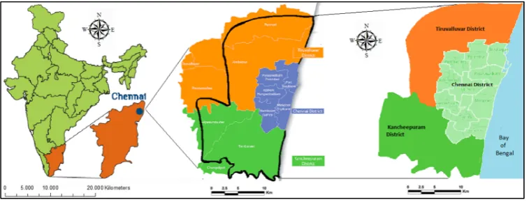
Chennai is the capital city of Tamilnadu, India, and gateway of south India (Figure 1). The geographical location of Chennai is 13.04°N 80.17°E with an elevation between 6m and 60m above the mean sea level. It covers an area of about 42,600ha. Due to the high urbanization in the Chennai district, most of the residential amenities, industries and factories, universities, and educational institutes are moving toward the periphery of Tiruvallur (North Chennai) and Kanchipuram (South Chennai) districts [21]. For this reason, this study also covers the 10km adjacent area of Chennai city (82,488.16ha) from Tiruvallur and Kanchipuram district for analyzing urban sprawl.
4
sites, such as monuments and ancient temples. The city is well engaged with trade, employment, and business. Chennai is also rich in natural resources [23]. As a result, the population has increased rapidly in the last two decades [18].
The city coastline is about 25.60km and has a lengthy natural urban beach (Marina beach) [24]. The city also has a dense forest, which is the only habitat of the Great Indian Horned Owls and home to spotted deer, mongoose, bonnet monkeys, and many species of insects, snakes, and birds [25]. The mangroves along the coastline, iluppai, caper, and vanni trees and trinicomalee teak are part of the city vegetation [11].
Figure 1. Location of the study area.
3. Data and methods
3.1 Data
Two decades of Landsat Thematic Mapper TM satellite images with 30m resolution for years 1991, 2003, and 2016 were used (Table 1). These Landsat data were downloaded without charge from the Unites States Geological Survey (USGS) portal [26] using a World Geodetic System (WGS) 1984 projection.
Table 1. Data description.
Date Sensor Path/Row Resolution Format
August 25th, 1991 Landsat-5 142/51 30m GeoTIFF
May 9th, 2003 Landsat-7 142/51 30m GeoTIFF
July 4th, 2016 Landsat-7 142/51 30m GeoTIFF
Preprints (www.preprints.org) | NOT PEER-REVIEWED | Posted: 5 January 2017 doi:10.20944/preprints201701.0023.v1
5
3.2 Satellite image pre-processing and land-use and land-cover mapping
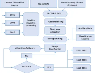
The availability of multi-temporal data obtained from the remote sensing techniques supports the development of change mapping and detection for land-use and land-cover (LULC) [9]. The LULC is mainly useful for environmental studies, studies on urban dynamics and urban sprawl modelling, and studies on sustainable development [27]. Therefore, the urban sprawl studies, as is the case with this research, should rely on updated terrain land-use and land-cover classification. Figure 2 shows the flow chart for image pre-processing and classification, and validation.
Figure 2. Methodology followed for image pre-processing, classification, and validation.
3.2.1 Image pre-processing
6
3.2.2 Image classification in R programming
Object-based classification in R programming is becoming more advantageous for classifying high-resolution satellite image at object level instead of pixel level [29]. Random forest (RF) classification is a machine learning algorithm adequate for object-based classification, which produces automatic and accurate results compared to other conventional classification methods [30]. We used RF package in R programming for land-use and land-cover classification [31]. Five land-use classes were extracted from the resulting image classification [32]. The categories and their corresponding classes are described in Table 2.
Table 2. Land-use and land-cover nomenclature.
No LULC classes Land uses included in the class
1 Water bodies Rivers, reservoir, lake, streams, open water, and ponds 2 Urban Residential, industries, IT sectors, private and government
buildings, roads, airport, and other related built-up areas 3 Agriculture Agriculture land and plantation
4 Bare land Dry land, non-irrigated lands, ready for construction, and real estate plots
5 Vegetation Forest and shrubs
The spatially and spatially-cohesive features on the ground are divided by running the segmentation algorithm in the ENVI feature extraction tool [33]. This segmentation process is used to locate several regions with maximum homogeneity. The feature in the region can be vegetation covers of parallel structure, appearance, and color. The segmentation algorithm reduces the heterogeneity of image features or objects for a given resolution [34]. The segmentation image from classified raster data is obtained by providing minimum and maximum threshold values of pixel and population of pixels that can be contained in a region.
3.2.3 Accuracy assessment
Accuracy assessment evaluates the performance of the image classification procedure [35]. This study used kappa coefficients [36] to analyze the accuracy of three-decade classified images. The producer data were obtained from Google Maps; thus, user and producer accuracies were calculated through a confusion matrix. The kappa coefficient index was calculated for the three
Preprints (www.preprints.org) | NOT PEER-REVIEWED | Posted: 5 January 2017 doi:10.20944/preprints201701.0023.v1
7
different date land-use classified images in eCognition Developer [37].
3.3 Spatiotemporal urban sprawl analysis
3.3.1 Urbanization analysis using spatial metrics
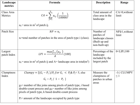
Different landscape metrics were calculated in FRAGSTATS software [38] to understand the pattern of urban growth from 1991 to 2016 (Table 3). These metrics were used to quantify and compute the spatial characteristics at different levels: patch level, class area level, and the complete landscape level. The selected landscape metrics were CA, NP, LPI, CLUMPY, AI, FRAC_AM, and CONTAG [39].
Table 3. Spatial metrics used in the study.
Landscape metrics
Formula Description Range
Class Area
Metrics = 1
10000
aij = area in m2 of patch ij.
Total amount of class area in the landscape
CA>0,without limit
Patch Size =
ni=total number of patches in the area of patch type i (class).
Number of patches of
landscape classes (Built up and non-built-up)
NP≥1,without limit
Largest
patch Index = (100)
aij = area in m2 of patch ij and A= landscape area in total(m2)
Percentage of the landscape
included by the largest patch
0<LIP≤100
Clumpiness
Index = [( − )/ < &
< 5, else − / 1 − ]
gii= number of like joins among pixels of patch type, i based double-count process and gik= number of like joins among pixels of patch type, k based double-count process
Pi= amount of the landscape occupied by patch type
Measure the clumpiness of patches in urban areas
8 Aggregation
Index = [ / ] (100)
gii= number of like joins among pixels of patch type, i based double-count process and maxgii=maximum number of like adjacencies among pixels of patch type
Calculates the adjacency between similar patch types
0 ≤ AI ≤ 100
Fractal Index Distribution
= [ ( / ) ]
aij = area in m2 of patch ij.
To measure area weighted mean patch fractal dimension 1 ≤ FRAC_AM≤2 Contagion
= [1 + [( ){ / }{ln( ) [
/ ]/2 ln( )]100
pi= amount of the landscape employed by patch type (i) class and gik= number of like joins among pixels of patch type, i and k based double-count process
m= number of patch classes (types) existing in the landscape
Defines the heterogeneity of a landscape
Percent<Cont agion≤100
3.3.2 Urbanization analysis using Renyi’s entropy
Renyi’s entropy was calculated to estimate urban sprawl between 1991 and 2016. This concept is used in information theory and image processing analysis such as information entropy [40]. To estimate the urban sprawl of Chennai city over three decades, the land-use and land-cover map was separated into two built-up and non-built-up classes and their spatial and temporal variations were taken into consideration.
Renyi´s entropy is based on knowledge theory and acts as an indicator of spatial dispersion or intensity to examine any geographic components [40]. We calculated Renyi’s entropy for each
period based on the total number of patches (N) in the LULC and their length (Pi). The extended
version of Shannon’s information defining a comprehensive entropy [41] of order Hα, where α ≥
0 and α≠ 0 is described as (1):
= ∑ (1)
Preprints (www.preprints.org) | NOT PEER-REVIEWED | Posted: 5 January 2017 doi:10.20944/preprints201701.0023.v1
9
The Renyi’s entropy values vary from 0, indicating very dense distribution in a selected region, to
1, indicating unequal distribution / dispersed across space [41]. 3.4 Urban growth model
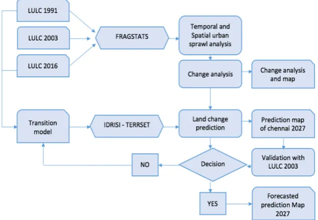
Land change modeler in IDRISI/TERRSET [42] was used to predict the urban growth of the study area in 2027. The land change modeling process consists of four steps: (1) urban change analysis, (2) transition modelling, (3) change prediction, and (4) validation. Figure 3 shows the methodology followed for change analysis and modelling.
Figure 3. Methodology applied for spatial and temporal analysis and modelling, and validation.
4. Results and Discussion
4.1 Land-use and land-cover classification and accuracy assessment
10
Figure 4. LULC of the three periods (1991, 2003, and 2016).
Preprints
(www.preprints.org) | NOT PEER-REVIEWED | Posted: 5 January 2017
doi:10.20944/preprints201701.0023.v1
Peer-reviewed version available at
Entropy
2017
,
19
, , 163;
11
Table 4. Summary of confusion matrix for the classified images 1991, 2003 and 2016.
Classes 1991 2003 2016
Producer Accuracy
User Accuracy
Producer Accuracy
User Accuracy
Producer Accuracy
User Accuracy
Urban 91.05 92.32 82.02 98.09 78.12 97.25
Vegetation 98.45 93.58 93.04 97.12 84.56 89.78
Agriculture 96.68 91.56 98.56 86.45 96.04 97.31
Water bodies 93.65 92.05 84.51 89.47 92.78 92.23
Bare land 92.01 94.02 94.03 88.12 76.05 95.77
Overall accuracy 92 97 91
Kappa 0.92 0.97 0.92
4.2 LULC changes and analysis
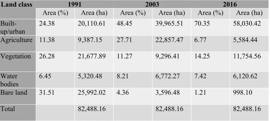
The LULC maps of three different periods were quantified and the results are in Table 5. The quantified result clearly shows that the study area has experienced a remarkable change among the land classes. From 1991 to 2016 the growth of built-up more than tripled, i.e. an increase of about 37,919.81ha. This transformation influenced several classes, especially the agriculture and vegetation land, which decreased about 3,802.70ha and 9,923.32ha respectively. The bare land also decreased around 30.3%, i.e. nearly 100%. The water bodies increased about 1,451.79ha between 1991 and 2003, but decreased slightly between 2003 and 2016 (about 651.65ha).
Table 5. Land-use and land-cover in percentage and hectares during the three periods.
Land class 1991 2003 2016
Area (%) Area (ha) Area (%) Area (ha) Area (%) Area (ha)
Built-up/urban
24.38 20,110.61 48.45 39,965.51 70.35 58,030.42
Agriculture 11.38 9,387.15 27.71 22,857.47 6.77 5,584.44 Vegetation 26.28 21,677.89 11.27 9,296.41 14.25 11,754.56
Water bodies
6.45 5,320.48 8.21 6,772.27 7.42 6,120.62
Bare land 31.51 25,992.02 4.36 3,596.48 1.21 998.10
12
4.3 Analysis of landscape metrics
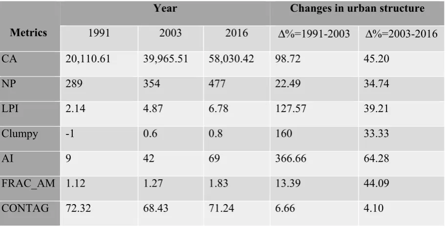
The spatial metrics were calculated with FRAGSTATS tool [38]. The values obtained and changes in percentage are in Table 6. The spatial variations and metrics were estimated for the built-up areas, indicating that the urban area increased by 98.72% between 1991 and 2003. Likewise, the built-up area between 2003 and 2016 also increased by 45.20%. When compared to 2003, the growth rate of urban area in 2016 is becoming slower (about 3%). The urban areas increased by 188.55% during the last three decades.
Patch size (NP) calculation helps to quantify the level of fragmentation, i.e. aggregation or disaggregation in the built-up landscape [16]. The number of patches has significantly increased (22.49%) between 1991 and 2003. Similarly, the NP increased about 37.74% between 2003 and 2016. The number of built-up patches noticeably increased in number during the last two decades. The patches at the center of the urban area were clumped after 2003 and more fragmented during 2003 and 2016.
The proportion of the landscape area covered by the largest urban patch is quantified by the Largest Patch Index (LPI) landscape metrics [18]. The LPI increased by 127% between 1991 and 2003. The higher value in the number of urban patches illustrates a denser urban growth, but it decreases moving away from the center, showing the existence of semi-urban or peri-urban fragmented urban patches. However, LPI increased by 39.21% from 2003 to 2016, indicating a compact urban growth and presence of new dispersed settlements.
In order to identify and examine the patch aggregation level, the clumpiness index was used. This landscape metric measures the clumpiness of urban patches [13]. The clumpiness in 1991 is -1, showing that the urban patch is maximally disaggregated. However, these values were 0.6 and 0.8 in 2003 and 2016, respectively, indicating that the urban patches are becoming aggregated or clumped. The patch clumpiness increased by 180% from 1991 to 2016, indicating that the urban patch became more clumped.
The aggregation index is computed from an adjacency matrix to measure the aggregation amount of the urban patches. The value of the aggregation index in 1991 shows the aggregation level as 9, indicating that the urban center is more clumped, and that the outskirts or suburbs have few patches. However in the following years (2003 and 2016) the suburbs and peripheral zone had a
Preprints (www.preprints.org) | NOT PEER-REVIEWED | Posted: 5 January 2017 doi:10.20944/preprints201701.0023.v1
13
highly fragmented progression and were more clumped in the city region. The patch aggregation in the urban structure clearly indicates that the city is becoming a more homogenous urban patch and that the suburbs are also developing with clumped patches as well as uneven patches. The growth of homogeneous and heterogeneous urban patches is destroying other classes such as vegetation, agriculture, and bare land, and transforming these landscapes into a single large urban patch.
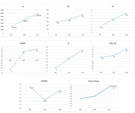
FRAC_AM increased between 1991 and 2003 as a result of contained urban growth with reasonable shape complexity (the values for this metric are marginally greater than 1). Nevertheless, the FRAC_AM value between 2003 and 2016 was 1.83, indicating that the landscape had a higher range of urban growth and more dispersed urban sprawl. The value between 2003 and 2016 has increased by 44.09%. The fall in the CONTAG value between 1991 and 2003 resulted from a higher fragmentation. However, this value increased slightly between 2003 and 2016 (4.10%) showing that the fragmented urban area is becoming denser. Figures 5 shows different temporal urban settlement growth signatures of spatial metrics.
Table 6. Landscape indices and changes in percentage.
Metrics
Year Changes in urban structure
1991 2003 2016 Δ%=1991-2003 Δ%=2003-2016
CA 20,110.61 39,965.51 58,030.42 98.72 45.20
NP 289 354 477 22.49 34.74
LPI 2.14 4.87 6.78 127.57 39.21
Clumpy -1 0.6 0.8 160 33.33
AI 9 42 69 366.66 64.28
FRAC_AM 1.12 1.27 1.83 13.39 44.09
14
Figure 5. Different temporal urban settlement growth signatures of spatial metrics.
4.4 Urban sprawl measurement using entropy
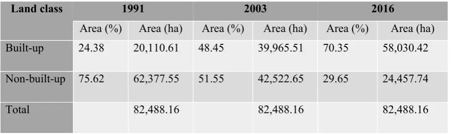
In order to estimate the sprawl and urbanization pattern during the last three decades, the LULC maps of Chennai and its peripheral district area were classified into non-built-up and built-up areas. The classified result shows that the Chennai area covered by the built-up area proportion was only 24.38% until 1991. This value has grown immensely, reaching 70.35% in 2016. The built-up and non-built-up area proportion has been switched during the last 25 years. The Renyi’s entropy calculation indicates that the Chennai city experienced high growth of the urban area between 1991 and 2016. The entropy value of the urban area in 1991 was 0.4, showing a moderate urban sprawl.
Preprints (www.preprints.org) | NOT PEER-REVIEWED | Posted: 5 January 2017 doi:10.20944/preprints201701.0023.v1
15
In 2003 the entropy value was 0.5, which is above the threshold value of 0.5, denoting a higher development of urban sprawl. In 2016 the entropy value was closer to 1, indicating a high urban sprawl level. Table 7 shows the built-up and non-built-up area in the Chennai city in 1991, 2003, and 2016.
Table 7. Built-up and non-built-up area in the Chennai city in 1991, 2003, and 2016.
Land class 1991 2003 2016
Area (%) Area (ha) Area (%) Area (ha) Area (%) Area (ha) Built-up 24.38 20,110.61 48.45 39,965.51 70.35 58,030.42 Non-built-up 75.62 62,377.55 51.55 42,522.65 29.65 24,457.74
Total 82,488.16 82,488.16 82,488.16
5.5 LULC changes and urban sprawl detection for year 2027
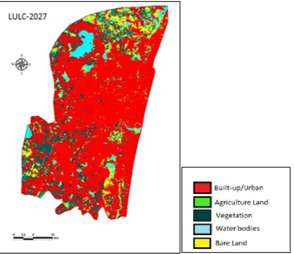
The land-use and land-cover prediction for the year 2027 was carried out after model validation, by confronting the 2016 LULC map with the kappa variations. The kappa value had an acceptable level of accuracy to predict the 2027 LULC map. The kappa values obtained were more than satisfactory (Kno = 82%, K location = 84% and Kquantity = 81%). The simulated 2027 land-use map and LULC transition between 1991 and 2016 and predicted LULC for the year 2027 are shown in Figures 6.
16
Figure 6. Simulated LULC map for the year 2027.
Table 8. Comparison of the LULC map of 2016 and predicted LULC map of Chennai 2027.
Land-use Class 2016 2027 Forecasted changes in 2027
in hectares in percentage Built-up/urban 58,030.42 70,836.76 12,805.58 22.06
Agriculture 5,584.44 701.35 -4,883.09 -87.44 Vegetation 11,754.56 3,961.66 -7,792.9 -66.29
Water bodies 6,120.62 5,420.62 -700 -11.43
Bare land 998.10 1,570.12 572.02 57.31
Total 82,488.16 82,488.16
In order to examine and visualize the spatial extension of the urban area in the predicted year (2027), the LULC of 2027 was classified into the built-up and non-built-up areas (Figure 7). The built-up areas amounted to 70.35% until 2016. This proportion increased to 85.87% in 2027. The Renyi’s entropy value of the predicted urban area in 2027 was 1.7, which is above the range value
Preprints (www.preprints.org) | NOT PEER-REVIEWED | Posted: 5 January 2017 doi:10.20944/preprints201701.0023.v1
17 of 1, indicating a complex growth of urban sprawl.
Figure 7. Classified LULC map for the year 2027.
5 Conclusions
The purpose of computing urban models for a period of time help us to understand the growth of the urban area and regulate the land transformation and sustainability [44]. The application of GIS, RS, and geospatial modelling tools enables the assessment and modelling of land-cover changes and the study of urban growth [45].
Land-use and land-cover maps of the Chennai city area for the years 1991, 2003, and 2016 were obtained using Random Forest classification with R programming. The computed maps provided a new perspective of the spatiotemporal distribution of the landscape in the study region. We found a fragmented urban growth in the outskirts of Chennai city, with the transformation of vegetation cover and agriculture land into settlements. The dense urbanization in the city region, quantified and analyzed using urban sprawl measurement and landscape metrics, raises challenges for sustainable urban planning and suitable land resource provision.
18
valuable urban vegetation and agriculture land and outward sprawling. The land changes around the urban center have to become denser and a reasonable amount of the urban expansion in Tiruvallur (North Chennai) and Kanchipuram (South Chennai) is also observed. This development is characterized by the decreasing largest patch index (LPI) and by the increase in the amount of urban patches (NP) in 2027.
The Chennai coastline had a remarkable urban growth between 1991 and 2016. Almost all the coastline of the study region is covered by urban settlements that negatively impact the mangrove forest [46] and the Savukku plantations [47]. This vegetation provides important ecosystem services, such as a natural shield from Tsunami, cyclones, and other ecological disasters [48]. Between 1991 and 2003 16.3% of agriculture and 15.01% of vegetation was transformed into urban/built-up, and 20.44% of agriculture land was lost between 2003 and 2016, while 30.3% of bare land became urban settlement during 1991 and 2003. The absence of involvement in agriculture by the population, the urban clumpiness in the city center, and the increasing population are the main reasons for such massive land transformation. The decreasing amount of vegetation and agriculture land will have negative environmental impacts, such as habitat loss for native species including Great Indian Horned Owls, spotted deer, mongoose, bonnet monkeys, and golden jackals [11]. Also, the degradation of forest and farm land leads directly to increases in city temperature and air pollution levels [49,50]. Recent studies already reveal that Chennai is one of the most highly air polluted cities in India [22].
The Entropy sprawl measurement indicates that the urban landscape had a high progress rate of urban sprawl and dispersion of urban growth between 1991 and 2016. This is directly and significantly influencing the urban fringe. The predicted entropy value for 2027 is 1.7, indicating a very high growth of urban sprawl.
Aggregated build-up, population growth, and land scarcity in the city are the reasons behind urban sprawl in the districts neighboring Chennai. Furthermore, increasing urban settlements also adds strain to sewage water disposal and waste management, both of which openly cause water and soil pollution [51]. Recent studies reveal that the threat of hydrological pollution of the Cooum river [52] and the coastal water in Chennai have been increasing due to the discharge of uncontrolled and non-treated sewage waters from domestic and commercial activities [53].The rapid growth of
Preprints (www.preprints.org) | NOT PEER-REVIEWED | Posted: 5 January 2017 doi:10.20944/preprints201701.0023.v1
19
urban area also poses a waste management problem, as everyday the city produces about 0.71kg of garbage per capita [54]. The recent investigation on waste disposal and management of Chennai city found that burning waste in Chennai's dump yards at Perungudi and Kodungaiyur creates severe soil and air pollution, which cause several health hazards, including respiratory disorders and the threat of cancer for nearby residents and animals [55].
The projected 2027 land-use and land-cover maps estimate an urban transition of 87% from agriculture land and 66% from vegetation, between 2016 and 2027. This projection and associated rapid transformation will most likely affect existing ecosystem services and the environment. At the same time, the bare land will increase at the expense of vegetation and agriculture classes. The growth and transformation of non-built-up area into the built-up area in the coming 11 years is expected to continue growing at an alarming rate.
The computation and modelling of urban growth patterns emphasize the need for well-judged land-use distribution and transformation, as well as the preparation of urban development policies giving importance to the sustainable deployment of natural resources. The land allocation strategy should conform to the land availability and capability classification of Chennai city to achieve sustainable urban expansion and development.
References
1. Stow, D. A.; Hope, A.; McGuire, D.; Verbyla, D.; Gamon, J.; Huemmrich, F.; Houston, S.; Racine, C.; Sturm, M.; Tape, K.; Hinzman, L.; Yoshikawa, K.; Tweedie, C.; Noyle, B.; Silapaswan, C.; Douglas, D.; Griffith, B.; Jia, G.; Epstein, H.; Walker, D.; Daeschner, S.; Petersen, A.; Zhou, L.; Myneni, R. Remote sensing of vegetation and land-cover change in Arctic Tundra Ecosystems. Remote Sens. Environ.2004, 89, 281–308.
2. Schafer, A.; Victor, D. G. The future mobility of the world population. Transp. Res. Part A Policy Pract.2000, 34, 171–205.
3. Lambin, E. F.; Turner, B. L.; Geist, H. J.; Agbola, S. B.; Angelsen, A.; Folke, C.; Bruce, J. W.; Coomes, O. T.; Dirzo, R.; George, P. S.; Homewood, K.; Imbernon, J.; Leemans, R.; Li, X.; Moran, E. F.; Mortimore, M.; Ramakrishnan, P. S.; Richards, J. F.; Steffen, W.; Stone, G. D.; Svedin, U.; Veldkamp, T. A. The causes of land-use and land-cover change : moving beyond the myths. 2001, 11, 261–269.
20
5. Padmanaban, R. C. Modelling the Transformation of Land use and Monitoring and Mapping of Environmental Impact with the help of Remote Sensing and GIS. Int. J. Adv. Remote Sens. GIS 2012, 1, 36–38.
6. Visalatchi, a; P, R. C. Land Use and Land Cover Mapping and Shore Line Changes Studies in Tuticorin Coastal Area Using Remote Sensing. Int. J. Adv. Remote Sens. GIS 2012, 1, 1–12. 7. Monishiya, B. G.; Padmanaban, R. C. Mapping and change detection analysis of marine resources in Tuicorin and Vembar group of Islands using remote sensing. Int. J. Adv. For. Sci. Manag.2012, 1, 1–16.
8. Megahed, Y.; Cabral, P.; Silva, J.; Caetano, M. Land Cover Mapping Analysis and Urban Growth Modelling Using Remote Sensing Techniques in Greater Cairo Region—Egypt. ISPRS Int. J. Geo-Information2015, 4, 1750–1769.
9. Zhang, Q.; Wang, J.; Peng, X.; Gong, P.; Shi, P. Urban built-up land change detection with road density and spectral information from multi-temporal Landsat TM data. Int. J. Remote Sens.
2002, 23, 3057–3078.
10. Rani, C. S. S.; Rema, M.; Deepa, R.; Premalatha, G.; Ravikumar, R.; Mohan, A.; Ramu, M.; Saroja, R.; Kayalvizhi, G.; Mohan, V. The Chennai Urban Population Study ( Cups ) -
Methodological Details – ( Cups Paper No . 1 ). 1999, 19.
11. Jayaprakash, M.; Senthil Kumar, R.; Giridharan, L.; Sujitha, S. B.; Sarkar, S. K.; Jonathan, M. P. Bioaccumulation of metals in fish species from water and sediments in macrotidal Ennore Creek, Chennai, SE coast of India: A metropolitan city effect. Ecotoxicol. Environ. Saf.2015,
120, 243–255.
12. Cabral, P.; Santos, J. A. J. A.; Augusto, G. Monitoring Urban Sprawl and the National Ecological Reserve in Sintra-Cascais, Portugal: Multiple OLS Linear Regression Model Evaluation. J. Urban Plan. Dev.2011, 137, 346–353.
13. Herold, M.; Goldstein, N. C.; Clarke, K. C. The spatiotemporal form of urban growth: Measurement, analysis and modeling. Remote Sens. Environ.2003, 86, 286–302.
14. De Oliveira Filho, F. J. B.; Metzger, J. P. Thresholds in landscape structure for three common deforestation patterns in the Brazilian Amazon. Landsc. Ecol.2006, 21, 1061–1073. 15. Luck, M.; Wu, J. G. A gradient analysis of urban landscape pattern: a case study from the Phoenix metropolitan region, Arizona, USA. Landsc. Ecol2002, 17, 327–340.
16. Jat, M. K.; Garg, P. K.; Khare, D. Monitoring and modelling of urban sprawl using remote sensing and GIS techniques. Int. J. Appl. Earth Obs. Geoinf.2008, 10, 26–43.
17. Cadenasso, M. L.; Pickett, S. T. A.; Schwarz, K. Spatial heterogeneity in urban ecosystems:
Preprints (www.preprints.org) | NOT PEER-REVIEWED | Posted: 5 January 2017 doi:10.20944/preprints201701.0023.v1
21
conceptualizing land cover and a framework for classification. Front. Ecol. Environ.2007, 5, 80–88.
18. Aithal, B. H.; Ramachandra, T. V. Visualization of Urban Growth Pattern in Chennai Using Geoinformatics and Spatial Metrics. J. Indian Soc. Remote Sens.2016, 44, 617–633.
19. Sudhira, H. S.; Ramachandra, T. V; Jagadish, K. S. Urban sprawl pattern recognition and modelling using GIS. Map India, 2003, New Delhi2003, 1–9.
20. Shafizadeh Moghadam, H.; Helbich, M. Spatiotemporal urbanization processes in the megacity of Mumbai, India: A Markov chains-cellular automata urban growth model. Appl. Geogr.2013, 40, 140–149.
21. Gowri, V. S.; Ramachandran, S.; Ramesh, R.; Pramiladevi, I. R. R.; Krishnaveni, K. Application of GIS in the study of mass transport of pollutants by Adyar and Cooum Rivers in Chennai, Tamilnadu. Environ. Monit. Assess.2008, 138, 41–49.
22. Chithra, V. S.; Shiva Nagendra, S. M. Indoor air quality investigations in a naturally ventilated school building located close to an urban roadway in Chennai, India. Build. Environ.
2012, 54, 159–167.
23. Gundimeda, H.; Sukhdev, P.; Sinha, R. K.; Sanyal, S. Natural resource accounting for Indian states - Illustrating the case of forest resources. Ecol. Econ.2007, 61, 635–649.
24. Arabindoo, P. “City of sand”: Stately Re-Imagination of Marina Beach in Chennai. Int. J. Urban Reg. Res.2011, 35, 379–401.
25. Walker, B. Disturbance, Resilience and Recovery: A Resilience Perspective on Landscape Dynamics; 2008.
26. Padmanaban, R. C.; Sudalaimuthu, K. Marine Fishery Information System and Aquaculture Site Selection Using Remote Sensing and GIS. Int. J. Adv. Remote Sens. GIS2012, 1, pp 20-33. 27. Khin Mar Yee; Khine Phoo Wai; Bak Jinhyung; Choi Chul Uong Land Use and Land Cover Mapping Based on Band Ratioing with Subpixel Classification by Support Vector Machine Techniques (A Case Study on Ngamoeyeik Dam Area, Yangon Region). J. Geol. Resour. Eng.
2016, 4, 127–133.
28. Harris Geospatial solutions Environment for Visualizing Image Analysis Software http://www.harrisgeospatial.com/ProductsandSolutions/GeospatialProducts/ENVI.aspx.
29. Walter, V. Object-based classification of remote sensing data for change detection. ISPRS J. Photogramm. Remote Sens.2004, 58, 225–238.
22
31. Vincenzi, S.; Zucchetta, M.; Franzoi, P.; Pellizzato, M.; Pranovi, F.; De Leo, G. A.; Torricelli, P. Application of a Random Forest algorithm to predict spatial distribution of the potential yield of Ruditapes Philippinarum in the Venice lagoon, Italy. Ecol. Modell.2011, 222, 1471–1478.
32. Zamyatin, A. V. V.; Afanasyev, A. A. A.; Cabral, P. Approach to the analysis of land cover dynamics using change detection and spatial stochastic modeling. Optoelectron. Instrum. Data Process.2015, 51, 354–363.
33. Lu, Y.; Michaels, J. E.; Member, S. Structural Health Monitoring Under Changing Environmental Conditions. 2009, 9, 1462–1471.
34. Pesaresi, M.; Benediktsson, J. A. A new approach for the morphological segmentation of high-resolution satellite imagery. IEEE Trans. Geosci. Remote Sens.2001, 39, 309–320. 35. Congalton, R. G. A review of assessing the accuracy of classifications of remotely sensed data. Remote Sens. Environ.1991, 37, 35–46.
36. Stehman, S. V. Estimating the Kappa coefficient and its variance under stratified random sampling. Photogramm. Eng. Remote Sens.1996, 62, 401–407.
37. Flanders, D.; Hall-Beyer, M.; Pereverzoff, J. Preliminary evaluation of eCognition object-based software for cut block delineation and feature extraction. Can. J. Remote Sens.2003, 29, 441–452.
38. UMass landscape ecology lab FRAGSTATS: Spatial Pattern Analysis Program for Categorical Maps http://www.umass.edu/landeco/research/fragstats/fragstats.html.
39. Herold, M.; Scepan, J.; Clarke, K. C. The use of remote sensing and landscape metrics to describe structures and changes in urban land uses. Environ. Plan. A2002, 34, 1443–1458. 40. Tsallis, C. Possible generalization of Boltzmann-Gibbs statistics. J. Stat. Phys.1988, 52, 479–487.
41. Drius, M.; Malavasi, M.; Acosta, A. T. R.; Ricotta, C.; Carranza, M. L. Boundary-based analysis for the assessment of coastal dune landscape integrity over time. Appl. Geogr.2013, 45, 41–48.
42. Clarks labs TerrSet Geospatial Monitoring and Modeling Software https://clarklabs.org/terrset/.
43. Binnig, N. Laureate & G. Cognition Network Technology http://www.ecognition.com/suite/ecognition-developer.
44. Burkhard, B.; Kroll, F.; Müller, F.; Windhorst, W. Landscapes’ capacities to provide
Preprints (www.preprints.org) | NOT PEER-REVIEWED | Posted: 5 January 2017 doi:10.20944/preprints201701.0023.v1
23
ecosystem services - A concept for land-cover based assessments. Landsc. Online2009, 15, 1– 22.
45. Tewolde, M. G.; Cabral, P. Urban sprawl analysis and modeling in Asmara, Eritrea. Remote Sens.2011, 3, 2148–2165.
46. Chaves, A. B.; Lakshumanan, C. Remote Sensing and GIS- Based Integrated Study and Analysis for Wetland Mangrove Restoration in Ennore Chennai Creek , South India . 2008, 685–690.
47. Tanaka, N. Vegetation bioshields for tsunami mitigation: Review of effectiveness, limitations, construction, and sustainable management. Landsc. Ecol. Eng.2009, 5, 71–79. 48. Kerr, A. M.; Baird, A. H.; Bhalla, R. S.; Srinivas, V. Reply to “Using remote sensing to assess the protective role of coastal woody vegetation against tsunami waves.” Int. J. Remote Sens.2009, 30, 3817–3820.
49. Dhorde, A.; Gadgil, A. Long-term temperature trends at four largest cities of India during the twentieth Century. J Ind Geophys Union2009, 13, 85–97.
50. Kim Oanh, N. T.; Upadhyay, N.; Zhuang, Y. H.; Hao, Z. P.; Murthy, D. V. S.; Lestari, P.; Villarin, J. T.; Chengchua, K.; Co, H. X.; Dung, N. T.; Lindgren, E. S. Particulate air pollution in six Asian cities: Spatial and temporal distributions, and associated sources. Atmos. Environ.
2006, 40, 3367–3380.
51. Raj chandar, R.; Kumar, R. Mapping and Analysis of Marine Pollution in Tuticorin Coastal Area Using Remote Sensing and GIS. 2012, 1, 34–48.
52. Giridharan, L.; Venugopal, T.; Jayaprakash, M. Evaluation of the seasonal variation on the geochemical parameters and quality assessment of the groundwater in the proximity of River Cooum, Chennai, India. Environ. Monit. Assess.2008, 143, 161–178.
53. Shanmugam, P.; Neelamani, S.; Ahn, Y. H.; Philip, L.; Hong, G. H. Assessment of the levels of coastal marine pollution of Chennai city, Southern India. Water Resour. Manag.2007, 21, 1187–1206.
54. Vasanthi, P.; Kaliappan, S.; Srinivasaraghavan, R. Impact of poor solid waste management on ground water. Environ. Monit. Assess.2008, 143, 227–238.
55. Raman, N.; Narayanan, D. S. Impact of Solid Waste Effect on Ground Water and Soil Quality Nearer To Pallavaram Solid Waste Landfill Site in Chennai. 2008, 1, 828–836.