Variational Methods for Control and Design of Bipedal Robot Models

(1)

for Control and Design of Bipedal Robot Models

Thesis by

David N. Pekarek

In Partial Fulfillment of the Requirements for the Degree of

Doctor of Philosophy

California Institute of Technology Pasadena, California

2010

(2)

(3)

Acknowledgments

Foremost, I wish to acknowledge and thank my advisor Jerrold E. Marsden. His kind-hearted guidance throughout my graduate studies has been an invaluable contribution to my academic and professional development. For this I am truly grateful.

I wish to thank the members of my thesis committee, Joel Burdick, Richard Murray, and Mathieu Desbrun. Their interaction and advice has certainly improved the quality and direction of my research. I would also like to thank additional Caltech faculty, John Doyle, Jim Beck, and David Boyd for their time and interest.

I have had so many postdocs and fellow graduate students make a positive impact on my stay at Caltech. In no particular order, I would like to acknowledge John Delacruz, Morgan Putnam, Noel du Toit, Glenn Garrett, Anne Dekas, John Matson, Andy Downard, Justus Brevik, Jeff Hanna, Dominic Rizzo, Nok Wongpiromsarn, Peter Trautman, Elisa Franco, Pablo Abad-Manterola, John Meier, Chris Kovalchick, Andrea Leonard, Nick Hudson, Michael Wolf, Julia Braman, Jeremy Ma, Tony Roy, Molei Tao, Ashley Moore, Philip du Toit, Ari Stern, Katalin Grubits, Nawaf Bou-Rabee, Sigrid Leyendecker, Marin Kobilarov, Sina Ober-Blöbaum, Andy Lamperski, and surely several others. Part of the joy of life at Caltech was a working environment that included each of them.

(4)

Certainly, I must acknowledge my parents, Charles and Kathy, my brothers, Joe and Will, and my grandparents, William and Mary. They have loved and supported me longer than anyone, regardless of my faults. I have also been supported by newer family members, my step parents, Mark and Margaret, sisters-in-law, Meeah and Andrea, step siblings, Leah and Spencer, and step grandfather, Pierre. The more the merrier.

(5)

Abstract

This thesis investigates nonsmooth mechanics using variational methods for the mod-eling, control, and design of bipedal robots.

The theory of Lagrangian mechanics is extended to capture a variety of nonsmooth collision behaviors in rigid body systems. Notably, a variational impact model is presented for the transition of constraints behavior that describes a biped switching stance feet at the conclusion of a step.

Next, discretizations of the impact mechanics are developed using the framework of variational discrete mechanics. The resulting variational collision integrators are consistent with the continuous time theory and have an underlying symplectic struc-ture.

In addition to their role as integrators, the discrete equations of motion captur-ing nonsmooth dynamics enable a direct method for trajectory optimization. Upon specifically defining the optimal control problem for nonsmooth systems, examples demonstrate this optimization method in the task of determining periodic gaits for two rigid body biped models.

(6)

List of Figures

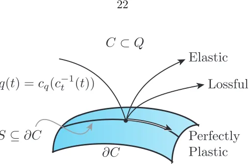
2.1 Trajectories q(t) representing a variety of collision models for free me-chanical systems. . . 22 2.2 Trajectoriesq(t)representing a variety of collision models for

holonomi-cally constrained mechanical systems. For simplicity, U =∂Rhas been

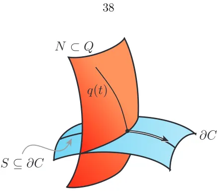
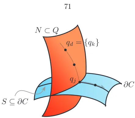
used in the perfectly plastic case. . . 25 2.3 A trajectory evolving through a transition of constraints. . . 38

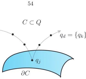
3.1 A discrete pathqdcapturing an elastic collision using discrete variational

jump conditions. . . 54 3.2 A holonomically constrained discrete path qd capturing an elastic

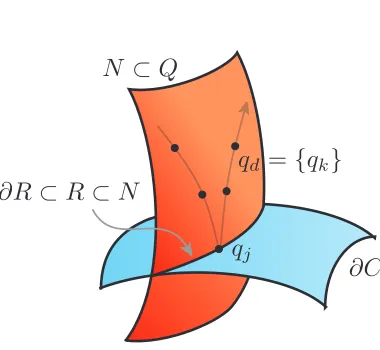
colli-sion using discrete variational jump conditions. . . 60 3.3 A discrete path qd capturing a transition of constraints using discrete

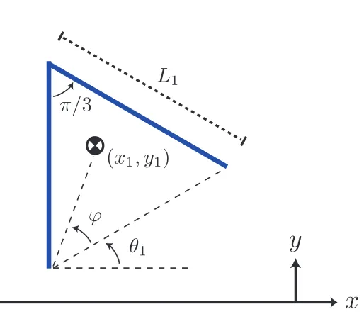
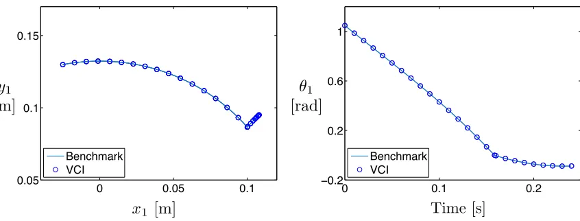
variational jump conditions. . . 71 3.4 A simple rigid body wedge model. . . 72 3.5 Evolution of the wedge’s center of mass in the plane (left) and orientation

over time (right) for the benchmark and VCI simulations. . . 74 3.6 Energy behavior and snapshots of the wedge progressing through a

tran-sition of constraints. The VCI accurately captures the loss in kinetic energy resulting from collision. The slowing of the system is reflected in the snapshots, which have been taken from the VCI simulation at even

(10)

4.1 A 4-link planar biped model. . . 83 4.2 Energy behavior and snapshots for one step of the planar biped’s locally

optimal periodic gait determined by DMOC. . . 85 4.3 A 4-link three-dimensional biped model with revolute joint knees and

a spherical joint hip. The triple (θ1, θ2, θ3) represents the ZYZ Euler angles of the body frame of first link with respect to the inertial frame, and (θ5, θ6, θ7)represents the ZYZ Euler angles of the body frame of the third link with respect to the body frame of the second. . . 86 4.4 Energy behavior and snapshots for one step of the three-dimensional

biped’s locally optimal periodic gait determined by DMOC. . . 88

5.1 The multilayered DD optimization scheme. . . 91 5.2 Progression of the “strawman” surrogate method in the outer loop of

DD. The optimal knee joint placement is determined in nine function evaluations. . . 95 5.3 Energy behavior and snapshots for one step of the locally optimal gait

(11)

Chapter 1

Introduction

It is an exciting time to study bipedal walking robots. Driven by nature’s examples in animals and humans alike, engineers and roboticists have persistently worked at synthetically capturing the abilities and efficiencies associated with legged locomotion. The last decade has seen a number high profile industry successes, notably Sony’s Qrio [35] and Honda’s Asimo [78], pushing the boundaries of robotic capabilites in walking. At first glance, the performance of these robots can make it seem that the major challenges in the field are foregone. In fact, these robots have given rise to new problems and have motivated new research directions.

(12)

1.1 Nonsmooth Mechanics

The dynamics of a walking robot are nonsmooth as a result of the change in ground contacts required to take a step. Assuming a model with no compliance at the contact, these dynamics require the modeling of rigid body impact mechanics. This is a task for which there are multiple approaches.

Perhaps the most popular approach is the use of measure differential inclusions. This tool extends the familiar framework of differential equations to allow measure-valued forces, namely impulses. Mathematically, differential inclusions were first con-sidered by Filippov [33, 34] and gained traction in the area of rigid body dynamics with the sweeping process of Moreau [70, 71]. The method is particularly popular for its ability to produce powerful existence and uniqueness results, notably Stewart’s work [85] resolving the paradox of Painlevé. A control theoretic approach for systems described with measure differential inclusions is provided by Brogliato [19, 21].

(13)

appears in numerous works [41, 26, 25, 4, 40, 44, 39, 38, 81, 76].

In this thesis, we make use of a third approach, variational nonsmooth mechanics. Similar to measure differential inclusions, this method can be considered as its own modeling framework or as a means to generate reset maps in the hybrid systems approach. The variational methodology used traces its roots to Young [87], and has been used in the context of rigid body impacts in [54, 23, 32]. The work of Fetecau et al. [32] features the symplectic structure underlying this description of impacts, one of the method’s main advantages. However, existence and uniqueness results are a significant challenge when using this method, an issue that remains deferred in this thesis.

1.2 Discrete Mechanics

Capturing nonsmooth mechanics with variational methods enables their representa-tion in discrete time as variarepresenta-tional integrators. An excellent account of variarepresenta-tional integrators and their derivation for standard smooth mechanics problems is provided in [42]. The geometric structure of variational integrators is discussed in the context of the discrete mechanics framework in Marsden and West [68]. This framework has been succesfully applied in describing a wide range of areas within mechanics: con-strained systems [68, 61, 59, 69], solid mechanics [57, 59], mechanical systems on Lie groups [16, 55], electromagnetics [83], and nonsmooth mechanics [32, 27].

(14)

these methods, but benefits from the discrete symplectic structure at its foundation. The discrete mechanics framework, in addition to developing variational integra-tors, provides a means to solve optimal control problems. First explored in Junge et al. [47], the method of discrete mechanics and optimal control (DMOC) recasts a standard optimal control problem as a finite-dimensional optimization problem. In doing so, the DMOC method fits in the class of direct methods for trajectory op-timization. A wealth of literature exists regarding solution methods for trajectory optimization, direct methods and otherwise. We highlight the surveys provided in [13, 12].

1.3 Design Optimization with Surrogates

(15)

of Booker et al. [15] has extended them to do so with the incorporation of pattern search steps.

1.4 Contributions and Thesis Outline

Chapter 2 provides a review of smooth mechanical systems, both free and holonomi-cally constrained, using a nonautonomous variational approach. This review sets the stage for the variational development of rigid body impact mechanics. Variational principles lead to nonsmooth dynamics for systems, both free and holonomically con-strained, undergoing elastic, inelastic, and perfectly plastic collisions. Dynamics are also derived for impacts causing a transition of constraints, the case that is pertinent for modeling walking. Additionally, the chapter makes use of null space descriptions [60, 10, 9] in the nonsmooth dynamics wherever possible. The merging of variational methodologies for constraints and nonsmooth behaviors is a notable contribution.

Chapter 3 extends all of the derivations from Chapter 2 to a discrete time setting. The resulting discrete time equations of motion are suitable for use as variational integrators. A nonautonomous approach is required in the variational methodology, but can also lead to infeasibility during integration. Hence, a discussion is main-tained to indicate when adaptive time stepping is advisable during integration. The development and demonstration of variational collision integrators is the primary contribution in this chapter.

(16)

dynamics is the first of its kind.

Chapter 5 addresses the task of design optimization for bipedal robots. Specifi-cally, the previous chapter’s DMOC results are leveraged in a search for design pa-rameters that reduce the cost of optimal control. A framework utilizing surrogate methods to sample and optimize design parameters is outlined. This framework is then demonstrated, utilizing the “strawman” surrogate method, in the task of design-ing the knee joint placement in a 4-link biped. This use of surrogate methods to optimize designs for improved optimal control is a notable contribution.

(17)

Chapter 2

Variational Collision Mechanics

In this chapter, we develop a framework by which variational mechanics describes a variety of collision behaviors in rigid body mechanical systems. We begin by re-viewing smooth mechanical systems, both free and holonomically constrained, in a nonautonomous setting. This lays the foundation necessary to explore collisions of constrained systems, and finally collisions allowing or even causing changes in system constraints. These behaviors are essential when describing the dynamics of bipedal robots.

2.1 Smooth Systems

Before delving into impact mechanics, we conduct a quick review of free and holo-nomically constrained Lagrangian mechanics. Examining these systems in a nonau-tonomous setting yields redundant results; however, we labor through this nonetheless in order to build familiarity with the approaches that will be applied in the nonsmooth case.

2.1.1 Free Systems

Consider a mechanical system with an n-dimensional configuration manifold Q, this

(18)

nonautonomous approach we consider a “time-like” variableτ on the interval[0,1]and define parameterizations of time and trajectories in configuration space as mappings

ct(τ) and cq(τ), respectively. More formally, consider thepath space

M=T_×Q([0,1], Q),

where

T={ct ∈C∞([0,1],R) | c"t>0 in[0,1]},

Q([0,1], Q) = {cq ∈C2([0,1], Q)}.

Notice that the elements c ! (ct, cq) in M do not just define paths on the

con-figuration manifold Q, but rather paths on an extended configuration manifold

Qe =R_×Q. For any pathc_∈MonQe, we can invert the parameterizationt=ct(τ) to recover an associated curve on Qin the time domain as

q(t) =cq(c−_t1(t)).

Noting that M is a smooth manifold, we define an extended action map on path

space _G¯ _:_M_→_R _as

¯

G(ct, cq) = ! 1

0 ¯

L(c(τ), c"(τ))dτ,

where we have introduced the extended Lagrangian _L¯ _:_{T Qe} _→_R_{defined as}

¯

L(c(τ), c"(τ)) =L

"

cq(τ),c

"

q(τ) c"

t(τ)

#

c"_t(τ).

Remark 2.1: Notice the factor of c"

t that appears in L¯ after the (autonomous)

La-grangian term. The inclusion of this term is such that a change of variables t=ct(τ)

(19)

the form

G(q) = ! ct(1)

ct(0)

L(q,q˙)dt.

This factor of c"

t will be pervasive in the future instances that we recast autonomous

concepts in the nonautonomous setting.

Finally, we define the second-order submanifold of Qe as

¨

Qe = $

d2_c

dτ2(0) ∈T(T Qe)| c: [0,1]→Qe is a C

2 _curve %

.

Now we have all of the necessary elements in place to describe variations of the action with respect to the path.

Theorem 2.1: Given a Ck _Lagrangian, _k _≥ ₂_{, there exists a unique} _Ck−2 _mapping

EL: ¨Qe→T∗Qe and a uniqueCk−1 _one-form_Θ

LonT Qe, such that for all variations

δc∈TcM of c we have:

dG¯(c)_·δc= ! 1

0

EL(c"")_·δc dτ + ΘL(c")·δcˆ (τ)

& & &1

0, (2.1.1)

where

EL(c"") = ' ∂L ∂qc " t− d dτ " ∂L ∂q˙

#( dcq+ ' d dτ " ∂L ∂q˙

c"q c"

t −

L

#(

dct,

ΘL(c") =

'

∂L ∂q˙ (

dcq₋

'

∂L ∂q˙

c" q c" t − L ( dct, ˆ

δc(τ) = ""

c(τ), ∂c ∂τ(τ)

#

,

"

δc(τ),∂δc ∂τ (τ)

##

.

As in [32], we term EL the Euler-Lagrange derivative and ΘL the Lagrangian

one-form. The latter of these expressions is consistent with the terminology in [67].

(20)

the action as

dG¯(c)·δc= ! 1

0 '

∂L ∂qδcq+

∂L ∂q˙

"_δc_"

q c"

t

−c

"

qδc"t

(c"

t)2

#(

c"_tdτ + ! 1

0

Lδc"_tdτ.

Using integration by parts on all instances of δc"

q = dτdδcq and δc"t = dτdδct produces

the desired result. !

Hamilton’s principle indicates that trajectories of the mechanical system will cor-respond with stationary points of the action. That is, a solution c _∈ M will yield

dG¯(c)_·δc= 0for variationsδc_∈TcMthat vanish at the boundaries0and1. Utilizing (2.1.1), we see that setting variations to zero at the boundaries eliminates the influ-ence of the ΘL(c") term, and it is sufficient for solutions to produce EL(c"") = 0 for

all τ ∈ (0,1). This yields the extended Euler-Lagrange equations, which, when

expressed in the time domain, take the form

∂L ∂q − d dt " ∂L ∂q˙

#

= 0 (2.1.2)

d dt

"

∂L ∂q˙q˙−L

#

= 0 (2.1.3)

for all t ∈(ct(0), ct(1)).

Remark 2.2: For a given q(t) satisfying the extended Euler-Lagrange equations, there actually exists an equivalence class of paths (ct, cq) such that q(t) = cq(c−t1(t)).

For a detailed explanation of how to quotient this redundancy out of the results, see [31].

Perhaps unsurprisingly, in (2.1.2), we have revealed the standard Euler-Lagrange equations one would deduce in the autonomous setting. Noting that the energy of a Lagrangian system is E = )∂L_∂_q_˙q˙−L*, (2.1.3) implies energy conservation. While

(21)

know it to be true of autonomous systems obeying (2.1.2) (see [68] or [32]). Thus, the additional variational machinery involved in using a nonautonomous approach on smooth systems has yielded one additional redundant equation. While this is somewhat unrewarding, we will see greater merits of this approach in Section 2.2 and beyond.

2.1.2 Holonomic Constraints

In many instances, we may encounter mechanical systems where it is necessary, or perhaps simply advantageous, to describe the system using constraints. In general, these constraints take a variety of forms and are often classified according to different fundamental structures and dependencies (see [7] for instance). Here, we will only consider holonomic constraints of the form g(q) = 0, where g : Q _→ Rm_, _{m < n}_,

is a constraint function for which 0 is assumed to be a regular value such that

N =g−1₍₀₎ _⊂_Q _{is a}_{constraint submanifold}_{. As we remain in a nonautonomous} setting, we will often view the above as an extended constraint function g¯ :

Qe →Rm defined byg¯(c) =g(cq)c"t(recall Remark 2.1), with an associated extended

constraint submanifold Ne = ¯g−1_{(0) =}_R_×_N _⊂_Qe_.

One of the most accessible and widely used methods to handle such systems is the introduction of Lagrange multipliers. This approach, using the Lagrange multiplier theorem to construct equivalent variational principles, will be our focus in the context of both smooth and nonsmooth trajectories. However, when possible, we will describe results in terms of the null space method [60, 10, 9], which falls into the general class of projection methods. As we will encounter its application repeatedly, we now explicitly state the Lagrange multiplier theorem.

Theorem 2.2: Consider a smooth manifold M and a functionΦ :M _→V mapping

(22)

¯

G(c)_{− (}cλ,Φ(c)). The following are equivalent: 1. c∈D is an extremum of G¯_|D;

2. (c, cλ)∈M×V is an extremum of G˜.

Proof: See [1]. !

Using the manifold structure of Ne, we can consider restrictions of the extended

Lagrangian of the form _L¯Ne _{= ¯}_L_|

T Ne. We will be comparing the dynamics of L¯Ne

resulting from an action principle on T_×Q([0,1], N) with the dynamics of an

aug-mented Lagrangian _L˜g¯ _: _T₍_Qe _× _Rm₎ _→ _R _{derived in the higher dimensional}

constrained coordinate path space

Mcc =T×Q([0,1], Q)×L,

where T and Q([0,1], Q) are as previously defined and L is the space of

square-integrable curves cλ : [0,1]_→Rm_.

Theorem 2.3: Given an extended Lagrangian system_L¯ _:_{T Q}_e _→_R_{with an extended} holonomic constraint g¯ : Qe _→ Rm_{, denote} _Qe_˜ ₌ _Qe_×_Rm_, _Ne _{= ¯}_g−1₍₀₎ _⊂ _Qe_{, and}

LNe ₌_L_|

T Ne. The following are equivalent:

1. c _∈ T _× Q([0,1], N) extremizes G¯Ne = ¯G_|T Ne and thus is a solution of the

extended Euler-Lagrange equations for_L¯Ne_;

2. (c, cλ) ∈ Mcc produces q(t) = cq(c−t1(t)) and λ(t) = cλ(c−t1(t)) satisfying the

extended constrained Euler-Lagrange equations

∂L ∂q −

d dt

"

∂L ∂q˙

# =

"

dg dq

#T

·λ (2.1.4)

d dt

"

∂L

∂q˙q˙−L+g·λ #

= 0 (2.1.5)

(23)

for all t_∈(ct(0), ct(1));

3. (c, cλ)_∈Mcc extremizesG˜(c, cλ) = ¯G(c)−(cλ,Φ(c))and hence solves the

Euler-Lagrange equations for the augmented Lagrangian _L˜¯g _:_T_Qe˜ _→_R _{defined by}

˜

L¯g₍_{c, c}

λ, c", c"λ) = ¯L(c, c")− (cλ,g¯(c)).

Proof: We readily apply Theorem 2.2. In the context of that theorem, the full space

M isM=T_×Q([0,1], Q), the function to be extremized isG¯ as defined in Subsection

2.1.1, and V =L with the L2 inner product. Set Φ : M → V as Φ(c)(τ) = ¯g(c(τ)) such that c _∈ T_×Q([0,1], N) if and only if Φ(c) = 0 (meaning ¯g(c(τ)) = 0 for all

τ ∈[0,1]). From this it follows D= Φ−1_{(0) =}_T_×_Q_([0_,_1]_{, N}_).

The first condition above corresponds precisely with the first condition in Theorem 2.2. That is,c∈Dis an extremum ofG¯_|D. By the Lagrange multiplier theorem, this

is equivalent to (c, cλ)∈ M ×V being an extremum of G˜(c, cλ) = ¯G(c)− (cλ,Φ(c)).

Identifying M _×V with Mcc and examining the particular form of G˜ : Mcc →R, we

see the augmented Lagrangian _L˜¯g _:_T_Qe_˜ _→_R _{emerge as}

˜

G(c, cλ) = ¯G(c)− (cλ,Φ(c))

= ! 1

0 ¯

L(c, c")dτ − ! 1

0

(cλ(τ),Φ(c)(τ))dτ

= ! 1

0 +_¯

L(c(τ), c"(τ))_{− (}cλ(τ),g¯(c(τ)))

,

dτ

= ! 1

0 ˜

L¯g(c(τ), cλ(τ), c"(τ), c"_λ(τ))dτ.

As(c, cλ) extremizesG˜(c, cλ), it is also a solution to the Euler-Lagrange equations for

˜

L¯g_{, satisfying the third condition. Finally, the second condition follows from this by}

solving dG˜ = 0 and casting the results in the time domain using the same process as

(24)

We note a few properties of the extended constrained Euler-Lagrange equations and their relation to the unconstrained set (2.1.2) and (2.1.3). We see that (2.1.4) parallels the momentum evolution (2.1.2), although now in the presence of constraint forces )dg

dq

*T

· λ. These forces maintain that the system remains on N, which is

signified by (2.1.6). Noting this condition, we also see that the constrained system’s energy, the conserved quantity in (2.1.5), is equivalent to the previously defined energy

E. This energy conservation equation, similar to (2.1.3), is redundant in this setting.

In another effort to prepare tools for our treatment of nonsmooth mechanics, we will reconsider the system above using the vakonomic method [58] on the “hidden” (or secondary) constraints [29] associated with g. These constraints are simply the

time-differentiated form of g(q) = 0; that is, f :T Q→Rm _{such that}

f(q,q˙) = dg

dq ·q˙= 0.

In the nonautonomous setting, and in accordance with Remark 2.1, we define an equivalentextended hidden constraint as _f¯_:_T₍_Qe₎_→_Rm _{of the form}

¯

f(c, c") =f

"

cq,c

"

q c"

t

#

c"_t

= dg

dq

& & &

cq·c

"

q.

Given that c"

t is strictly positive, f = 0 if and only if f¯= 0. One important property

that will allow us to draw parallels between the usage of the holonomic constraint g

and the hidden constraintf is

dg dq =

∂f

∂q˙. (2.1.7)

Remark 2.3: The original constraint g(q) = 0 and the hidden constraint f(q,q˙) =

0 differ slightly in their respective constraint submanifolds. See that f−1₍₀₎ _{is the} space of paths satisfying d

(25)

t. We cannot guarantee that this space is N, or even a submanifold at all, without

the condition g(q(ct(0))) = 0. We will assume this condition henceforth and thus

f−1_{(0) =}_N _∈_Q_.

We should state that the vakonomic method, often mentioned in the context of nonholonomic constraints onT Q, is often disregarded for the more favorable

nonholo-nomic method [14]. However, in [58], it is shown that these methods are equivalent when applied to an integrable (i.e., holonomic) constraint. We show in the nonau-tonomous case that the vakonomic method producescq and ct equivalent to those in

Theorem 2.3.

Theorem 2.4: Given an extended Lagrangian system_L¯ _:_{T Q}_e _→_R_{with an extended} holonomic constraint ¯g : Qe _→ Rm _{and its associated extended hidden constraint}

¯

f : Qe _→ Rm_{, denote} _Qe_˜ ₌ _Qe _×_Rm_, _Ne _{= ¯}_f−1₍₀₎ _⊂ _Qe_{, and} _LNe ₌ _L_|

T Ne. The

following are equivalent:

1. c _∈ T _× Q([0,1], N) extremizes G¯Ne _{and thus is a solution of the extended}

Euler-Lagrange equations for _L¯Ne_;

2. (c, cλ) ∈ Mcc produces q(t) = cq(c−t1(t)) and λ(t) = cλ(c−t1(t)) satisfying the

vakonomic extended constrained Euler-Lagrange equations

∂L ∂q −

d dt

"

∂L ∂q˙

#

=₋

"

df dq˙

#T

·λ˙ (2.1.8) d

dt

"

∂L ∂q˙q˙−

"

df dq˙q˙

#

·λ₋L+f _·λ

#

= 0 (2.1.9)

f = 0, (2.1.10)

for all t_∈(ct(0), ct(1));

(26)

Euler-Lagrange equations for the augmented Lagrangian _L˜f _:_T_Qe_˜ _→_R _{defined by}

˜

Lf¯(c, cλ, c", c"_λ) = ¯L(c, c")− (cλ,f¯(c, c")).

Proof: The proof of this theorem follows identically the structure of the proof for the previous Theorem 2.3. The only difference is in the form of Φ : M → V, which

is now Φ(c)(τ) = ¯f(c(τ), c"₍_τ₎₎_{. Again, the Lagrange multiplier theorem provides}

equivalence of the first and third conditions, and here the augmented Lagrangian appears as _L˜_f¯

(c, cλ, c"_{, c}"

λ) = ¯L(c, c")− (cλ,f¯(c, c")).

The Euler-Lagrange equations associated with _L˜_f¯

take a slightly more complex form in this case. To see their derivation, examine thatdG˜ = 0 implies

0 = ! 1

0 '

EL(c"")_· δc

c"

t −

cλ· ∂f

∂qδcq−cλ· ∂f ∂q˙

"_δc"

q c"

t −

c"_qδc"_t

(c"

t)2

#

−f δcλ−cλ·f δc"

t c"

t

(

c"_tdτ

= ! 1

0 '"

∂L ∂q −cλ·

∂f ∂q

#

c"_t− d

dτ

"

∂L ∂q˙ −cλ·

∂f ∂q˙

#(

δcqdτ + ! 1

0

−f c"_tδcλdτ

+ ! 1 0 ' d dτ "" ∂L ∂q˙ −cλ·

∂f ∂q˙

#_c"

q c"

t −

L+cλ_·f

#(

δctdτ

+ '

∂L ∂q˙ −cλ·

∂f ∂q˙

(

δcq&&_&1

0+ '"

∂L ∂q˙ −cλ·

∂f ∂q˙

#_c"

q c"

t −

L+cλ _·f

(

δct&&_&1

0,

where·has been used as shorthand for the inner product. The expressions above fully define the Euler-Lagrange derivative and the Lagrangian one-form for the augmented Lagrangian _L˜_f¯

. For future reference, we record their definitions here as

-EL(c"", c""_λ) = '"

∂L ∂q −cλ·

∂f ∂q

#

c"_t₋ d dτ

"

∂L ∂q˙ −cλ·

∂f ∂q˙

#(

dcq

+ [−f c"_t]dcλ+ '

d dτ

"

∂L ∂q˙

c" q c" t −L #( dct (2.1.11)

Θ˜_Lf¯(c", c"_λ) =

'

∂L ∂q˙ −cλ ·

∂f ∂q˙

(

dcq− '"

∂L ∂q˙ −cλ·

∂f ∂q˙

#_c_"

q c"

t

−L+cλ ·f

(

dct (2.1.12)

Requiring that-EL(c""_{, c}""

(27)

domain provides (2.1.8), (2.1.9), and (2.1.10). In the final steps, the dcq terms

con-tainingf are collected and simplified as

−λ· ∂f

∂q − d dt

"

−λ· ∂f

∂q˙ #

=−λ· ∂f

∂q + ˙λ· ∂f ∂q˙ +λ·

∂2_f

∂q∂q˙q˙

= ˙λ· ∂f

∂q˙.

This cancellation produces the right-hand side of (2.1.8). !

Corollary 2.1: The path (c, cλ) ∈ Mcc satisfies the extended constrained

Euler-Lagrange equations if and only if there exists c˘λ ∈ L such that (c,c˘λ)∈ Mcc satisfies

the vakonomic extended constrained Euler-Lagrange equations.

Proof: By Theorems 2.3 and 2.4, the given statements are each equivalent to the condition: c_∈T_×Q([0,1], N)is a solution to the extended Euler-Lagrange equations for the restricted Lagrangian, _L¯Ne_{. Hence, they too are equivalent.}

!

Our results in the vakonomic case are nearly identical to the previous results (2.1.4), (2.1.5), and (2.1.6). Equation (2.1.8) is a momentum evolution equation with constraint forces, and noting the property (2.1.7) we see that these forces take nearly an identical form to those in (2.1.4) (there is just −λ˙ in place of the former λ).

Remark 2.3 has already mentioned the equivalence between the respective constraint equations (2.1.6) and (2.1.10). Finally, noting that f is linear in q˙, we have

∂f ∂q˙q˙=f,

such that (2.1.9) amounts to conservation of the unconstrained energy E.

Momentarily disregarding the redundant energy equations (2.1.5) and (2.1.9), each set of the paired equations (2.1.4), (2.1.6) and (2.1.8), (2.1.10) has the structure of an

(28)

(q, λ). The dimension of these systems should be somewhat disconcerting considering that they are capturing(n₋m)-dimensional dynamics on the submanifold N. Using

the null space method [61], we can reduce the dimension of the DAEs and eliminate the presence of any Lagrange multipliersλ.

We introduce the concept of ann×(n−m)null space matrix P(q)with(n−m) columns that form a basis ofTqN such thatP(q) :Rn−m →TqN. The term null space

matrix is derived from the property of P(q)that

range(P(q)) = null "

∂g ∂q(q)

#

=TqN. (2.1.13)

Note that there is no unique basis for TqN and hence P(q) is in general not unique.

However, (2.1.13) is a necessary and sufficient condition to define a null space matrix. Any P(q) satisfying this condition can be used as a projection on the DAEs (2.1.4) and (2.1.6) as follows

PT(q) '

∂L ∂q −

d dt

"

∂L ∂q˙

#(

= 0, (2.1.14)

g = 0, (2.1.15)

for all t _∈ (ct(0), ct(1)). Recalling (2.1.7), the same projection applies to the vako-nomic equations (2.1.8) and (2.1.10) which results in the DAEs above, just with

f = 0 in place of the equivalent condition (2.1.15). The DAEs (2.1.14) and (2.1.15) are equivalent to (2.1.4), (2.1.6) and (2.1.8), (2.1.10), but are only n-dimensional.

This is still higher than the dimension of the constrained dynamics, (n−m), but is

equivalent to the dimension of the constrained coordinates q. A lower dimensional

(29)

2.1.3 External Forcing

In this section, we study a generalization of the extended Euler-Lagrange equations for mechanical systems with external forces (e.g., friction, damping, or control forces). Adding the virtual work of such forces into our variational arguments marks a de-parture from Hamilton’s principle and to the Lagrange-d’Alembert principle. Here, we demonstrate this for the simplest case, the free systems of Subsection 2.1.1. How-ever, the following arguments readily apply to any of the variational principles in this chapter.

As in [67], we define anexterior force field as a fiber-preserving mapF :T Qe →

T∗Qe over the identity. Following Remark 2.1, we write this in coordinates a

F : (c, c")_→(c, F(c, c")c"_t).

Appending the virtual work of F = (Ft, Fq) to our previous Hamilton’s principle for free systems yields theintegral Lagrange-d’Alembert principle

δ

! 1

0

L

"

cq(τ),c

"

q(τ) c"

t(τ)

#

c"_t(τ)dτ+ ! 1

0

F(c(τ), c"(τ))_·δc dτ = 0,

where, as before, variations δc ∈ TcM vanish at the boundaries. Taking variations

of the action as in Subsection 2.1.1, we see the condition above is equivalent to the

extended forced Euler-Lagrange equations

∂L ∂q − d dt " ∂L ∂q˙

#

=−Fq, (2.1.16)

d dt

"

∂L ∂q˙q˙−L

#

=−Ft, (2.1.17)

for all t _∈ (ct(0), ct(1)). As a direct consequence of the energy evolution equation

(30)

between Fq and Ft. This relation appears as

Ft=−d

dt

"

∂L ∂q˙q˙−L

#

=−d

dt

"

∂L ∂q˙

# ˙

q− ∂L

∂q˙q¨+

∂L ∂q˙q¨+

∂L ∂q˙q˙

= "

−Fq− ∂L

∂q

# ˙

q+ ∂L

∂qq˙

=−Fqq.˙

Though mathematically the freedom exists to define forces (Ft, Fq) that violate this

condition, physically this would defy the conservation of mechanical energy.

2.2 Elastic Collisions

We now extend the concepts and variational principles in Section 2.1 to a nons-mooth setting. As discussed in [20], there are primarily two qualitatively different approaches for describing nonsmooth mechanics with variational principles. The first involves modifications to the path space [54] such that one takes variations over curves with isolated points of diminished smoothness or continuity. The second uses modi-fications to the variational principle itself [23] to include impulsive forces at certain configurations. We will be utilizing the former approach, mainly following the nota-tion and methods of [32]. First, we handle the most basic of nonsmooth behaviors, the energy-conserving elastic collision.

2.2.1 Free Systems

To model an unconstrained mechanical system undergoing an elastic collision, we keep our definitions ofQ,Qe,L,L¯, andG¯ from Section 2.1. Furthermore, we defineC _⊂Q,

(31)

that do not intersect any contact surface). The boundary of C, denoted ∂C, defines

the set of contact configurations.

Remark 2.4: Note that this definition of the set contact configurations implies that it is of codimension 1 relative to the set admissible configurations. This is in agreement with a point contact assumption. Cases of higher codimension, such as the case when multiple contacts are made at once, are excluded.

Nonautonomous trajectories of the above model belong to a nonsmooth path space defined by

Mns=T×Qns([0,1], τi, ∂C, Q),

where T remains as previously defined and

Qns([0,1], τi, ∂C, Q) ={cq : [0,1]→Q | cq is C0, piecewise C2,

∃ one singularity incq(τ) atτi, cq(τi)∈∂C}.

While the proof is excluded here, [32] shows that Mns is in fact a smooth manifold.

This path space allows for variations of the collision time ct(τi) while fixing the mo-ment of impact in τ-space. This property will be extremely useful in the variational

arguments to come, and indicates the utility of the nonautonomous approach in han-dling nonsmooth problems. The trajectory labeled “Elastic” in Figure 2.1 depicts an autonomous trajectoryq(t), derived from a path (ct, cq)∈Mns, that is subject to the

elastic collision model derived below.

Remark 2.5: While the path space definition does not explicitly exclude the possi-bility, we will assume that q˙ is not tangential to the contact set ∂C at τ_i− and τ_i+.

(32)

Figure 2.1: Trajectories q(t) representing a variety of collision models for free me-chanical systems.

With smoothness properties allowing for the implementation of variational cal-culus, we return to examining variations of the extended action map. Due to the singularity in cq (c"_q(τi) does not exist), the action integral must be split at τi and

integration by parts applied to each of the two resulting integrals. This results in the following for any δc_∈TcMns,

d_G¯₍_c₎_·_δc₌! τi 0

EL(c"")·δc dτ + ! 1

τi

EL(c"")·δc dτ

+ ΘL(c")

& & &τ

− i

0 · ˆ

δc(τ) + ΘL(c")

& & &1

τ_i+·

ˆ

δc(τ).

In the application of Hamilton’s principle to the varied action above, the integral terms imply the system obeys the extended Euler-Lagrange equations (2.1.2) and (2.1.3) for all t _∈ (ct(0), ct(τi))_∪(ct(τi), ct(1)). That is, the behavior of the system

away from the point of impact does not change from the smooth case. To determine the behavior at impact, notice variations δc still vanish at the boundaries 0 and 1 but not necessarily at τi. Hence the behavior of the Lagrangian one-form at τi has

(33)

impact. These conditions are

'

∂L

∂q˙dq−E dt (ct(τ_i+)

ct(τ_i−)

= 0, (2.2.1)

onT Qe_|(R_×∂C). To be exact, we say that an equality of forms holds “on” a particular tangent space if the equation holds upon contraction with any vector in that tangent space. This means the condition above could be written more formally as

∂L ∂q˙ & & &

ct(τ_i+)·vq =

∂L ∂q˙ & & &

ct(τ_i−)·vq, −E&&_&

ct(τ_i+)·vt =−E & & &

ct(τ_i−)·vt,

for all v = (vt,vq) ∈ T Qe|(R×∂C). As we will continually express jump conditions

using the equality of forms, it will be useful to retain this underlying meaning. Noting the tangent space in which it applies, (2.2.1) indicates both conservation of energy and conservation of momentum tangent to ∂C across the moment of impact.

These jump conditions provide no information regarding the momentum normal to

∂C, which we know is impulsively changing at impact in order for the system to

remain in the set of admissible configurations C.

Remark 2.6: The jump conditions defined in (2.2.1) admit the trivial solution

∂L ∂q˙ & & &

ct(τ_i+)=

∂L ∂q˙ & & &

ct(τ_i−),

but we readily disregard this as it yields inadmissible configurations q(t) ∈/ C for ct(τ)> ct(τi).

Geometrically speaking, we could express the momentum jump condition in (2.2.1) as

i∗

"

∂L ∂q˙ & & &τ

+ i

τ_i−

(34)

where i∗ _: _T∗_Q _→ _T∗_∂C _{is the cotangent lift of the embedding} _i _: _∂C _→ _Q_{. To}

formulate this condition in terms of the null space matrices of Subsection 2.1.2, let us assume (for notational purposes) that the manifold ∂C can be expressed as the

level set g_∂C−1(0) of some function g∂C :Q→R. Then, if we define ann×(n−1)null space matrix P∂C(q) :Rn−1 _→_Tq∂C _{that satisfies (2.1.13) for} _g ₌_g∂C _and _N ₌_∂C_, we can express the momentum jump condition as

P_∂CT (q) '

∂L ∂q˙

(ct(τ_i+)

ct(τ_i−)

= 0. (2.2.2)

Essentially with P∂C(q) as defined above, its transpose provides a mapping PT ∂C(q) : Tq∗Q → Tq∗∂C. We will maintain this use of the null space notation in our jump

conditions for the constrained cases ahead.

2.2.2 Holonomic Constraints

To model a holonomically constrained mechanical system undergoing an elastic col-lision we retain all of the notation and definitions from Subsections 2.1.2 and 2.2.1. We assume that R = (N _∩C) _⊂ Q is a submanifold with boundary defining the

set of constrained admissible configurations that lie in C and satisfy the

holo-nomic constraint g. In the nonautonomous setting, we will make regular reference

to Re =R×R. Furthermore, we assume the set of constrained contact

configu-rations ∂R, the boundary and a submanifold of R, is a submanifold of ∂C as well.

These manifolds, as well as a constrained trajectory undergoing an elastic collision (labeled “Elastic”), are shown in Figure 2.2. Finally, we assume at all points of con-tact q_∈∂R the manifolds R and ∂C are not tangential, i.e., the tangent spacesTqR

and Tq∂C are not equivalent nor is either a subset of the other. This assumption is

similar to the condition assumed in Remark 2.5.

(35)

Figure 2.2: Trajectories q(t) representing a variety of collision models for holonomi-cally constrained mechanical systems. For simplicity, U =∂R has been used in the

perfectly plastic case.

path space of the form

M"_ccns=M"_ns_×L,

where L is as previously defined and M"_ns = T _× Qns([0,1], τi, ∂R, Q). Note that

Qns([0,1], τi, ∂R, Q) uses our previous definition of Qns([0,1], τi, ∂C, Q), but replaces ∂C with ∂R. The path space M"_ccns restricts the point of contact to lie in ∂R unlike

the more general Mccns = Mns×L, which would only restrict it to ∂C. The choice

between these two definitions is a subtle issue, one we will revisit later. For now, we give the following theorem relating the nonsmooth dynamics of _L¯Re _{= ¯}_L_|

T Re

resulting from an action principle on T_×Qns([0,1], τi, ∂R, N) with the dynamics of

the augmented Lagrangian_L˜ _:_T₍_Qe_×_Rm₎_→_R _on_M"

ccns.

Theorem 2.5: Given an extended Lagrangian system_L¯ _:_{T Qe} _→_R_{on an admissible} set C, with a contact set ∂C, subject to an extended hidden constraint f¯: Qe →Rm

associated with an extended holonomic constraint¯g :Qe→Rm, denoteNe= ¯f−1(0)⊂ Qe, Re=R_×(N_∩C), and LRe ₌_L_|

(36)

1. c _∈ T_×Qns([0,1], τi, ∂R, N) extremizes G¯Re and thus is a solution of the

ex-tended Euler-Lagrange equations and variational jump conditions associated with _L¯Re_;

2. (c, cλ) ∈ M"_ccns produces q(t) = cq(ct−1(t)) and λ(t) = cλ(c−t1(t)) satisfying the

vakonomic extended constrained Euler-Lagrange equations for allt_∈(ct(0), ct(τi−))∩

(ct(τ_i+), ct(1)), as well as the variational jump conditions

'

∂L

ct(τ_i−)

= 0, (2.2.3)

onT Qe_|(R_×∂R).

3. (c, cλ) ∈ M"_ccns extremizes G˜(c, cλ) = ¯G(c)− (cλ,Φ(c)) and hence solves the Euler-Lagrange equations for the augmented Lagrangian_L˜_f¯

:T(Qe×Rm)→R

defined by

˜

Lf¯(c, cλ, c", c"_λ) = ¯L(c, c")_{− (}cλ,f¯(c, c")₎.

Proof: In the context of Theorem 2.2, our full space M is M"_ns. Keep in mind the

distinction between this space andMns; paths in this full space cannot stray from∂R

at the point of contact. The function to be extremized is_G¯ _{as defined in Subsection} 2.1.1, and again V = L with the L2 inner product. Set Φ : M → V as Φ(c)(τ) =

¯

f(c(τ)) such that for paths c in the full space, we have c∈ T_×Qns([0,1], τi, ∂R, N)

if and only if Φ(c) = 0. Hence, we have D= Φ−1_{(0) =}_T_×_Q

ns([0,1], τi, ∂R, N).

The first condition and third conditions are equivalent by Theorem 2.2. That is, c _∈ D extremizing G¯_|D is equivalent to (c, cλ) ∈ M ×V extremizing G˜(c, cλ) =

¯

G(c)_{− (}cλ,Φ(c)). Identifying M _×V with M"_ccns, the structure of G˜ : M"_ccns _→ R

(37)

integral such that variations of _G˜₍_{c, cλ}₎ _{have the form}

d_G˜₍_{c, cλ}₎_·_δc₌! τi 0

-EL(c"", c""_λ)·δ(c, cλ)dτ + ! 1

τi

-EL(c"", c""_λ)·δ(c, cλ)dτ

+ Θ_L˜f¯(c", c"_λ)

& & &τ − i 0 · ˆ

δ(c(τ), cλ(τ)) + Θ_L˜f¯(c", c"_λ)

& & &1

τ_i+·

ˆ

δ(c(τ), cλ(τ)).

The integral terms imply that the system obeys the vakonomic extended constrained Euler-Lagrange equations in the smooth regimet _∈(ct(0), ct(τi))_∪(ct(τi), ct(1)). Fur-thermore, the Lagrangian one-form terms atτi imply the jump conditions (expressed

in the time domain)

."

∂L ∂q˙ −

"

∂f ∂q˙

#T

·λ

#

dq

/ct(τ_i+)

ct(τ_i−) = 0,

onT Q_|∂R,and

."

∂L ∂q˙q˙−

"

∂f ∂q˙q˙

#

·λ₋L+f _·λ

#

dt

/ct(τ_i+)

ct(τ_i−) = 0,

on TR. Noting that the columns of )∂f_∂_q_˙*T are normal to T ∂R, the constraint term

in the momentum balance is negligible. Using the linearity of f with respect to q˙, the energy balance reduces to the conservation of E. Hence, the above conditions are

equivalent to those presented in (2.2.3). !

Remark 2.7: In the smooth case, the constraint condition Φ(c) = 0 simply meant ¯

f(c(τ)) = 0for allτ ∈[0,1]. In the nonsmooth case above, this is not precisely true as

the singularity atτi meansf¯(c(τ))does not exist there. In this case, we take Φ(c) = 0 to mean _f¯₍_c₍_τ+_{)) = 0} _and _f_¯₍_c₍_τ−_{)) = 0} _{for all} _τ _∈ _[0_,_1]_{. With this definition, it is}

in fact true Φ−1_{(0) =}_T_×_Q

ns([0,1], τi, ∂R, N).

(38)

which not only admits impulsive changes in momentum normal to ∂C as before,

but normal to R as well. That is, at impact, the system may be subject to both

impulsive contact forces and impulsive constraint forces. These forces must yield ¯

f(c(τ_i+)) = 0, which one might view as being implicitly appended to the jump

con-ditions since f = 0 must hold on t ∈(ct(τ_i+), ct(1)). Without this condition, we have

(q(ct(τ_i+)),q˙(ct(τ_i+))) ∈/ T R and the system has not been initialized in a way that

the DAEs (2.1.8) and (2.1.10) can be solved for t _∈ (ct(τi+), ct(1)). Though it was

not mentioned, a similar condition _f¯₍_c_{(0)) = 0} _{was implicit during our usage of the} vakonomic method in the smooth case.

Remark 2.8: It may be possible to develop results similar to Theorem 2.5 using a variational principle on Mccns, with Mns as the full space M. We have avoided this

choice due to its consequences regarding the structure of the Lagrange multipliers cλ.

UsingMnswould result in the jump conditions containing a momentum balance on T ∂C rather than on T ∂R. In the general case, impacts include impulsive constraint

forces normal to R and thus jump conditions on T ∂C may require impulsive cλ at

τi. Though the issue has been explored [74], impulsive generalized functions or, more

properly, distributions do not in general admit an inner product. Without belonging to an inner product space, cλ would no longer meet the necessary conditions of Theorem

2.2.

As a final note, the Lagrange multipliers cλ in our analysis are discontinuous but

not impulsive at τi and thus still satisfycλ ∈L.

To formulate the jump condition (2.2.3) in terms of a null space matrix, let us assume that the manifold∂Rcan be expressed as the level setg−_∂R1(0)of some function

(39)

(rather thang and N), we can express the momentum jump condition as

P_∂RT (q) '

∂L ∂q˙

(ct(τ_i+)

ct(τ_i−)

= 0. (2.2.4)

This in combination with E_|ct(τi+)

ct(τ_i−) = 0 is equivalent to (2.2.3).

2.3 Forced and Lossful Collisions

This section extends the previous variational methods to include work done at impact. Though the framework we consider could be used to model any type of instantaneous forces at the instant τi, we are primarily interested in capturing energy losses due to

friction and other sources of dissipation.

2.3.1 Free Systems

Following the structure of Subsection 2.1.3, we define a contact force field F∂C _:

T Qe|(R×∂C) → T∗₍_R_× _∂C₎ _{to model nonconservative impulsive forcing during}

collisions. As with the exterior force F, the force field F∂C _{= (}_F∂C

t , Fq∂C) has a time

component on the T∗Rportion of the cotangent bundle ofT Qe. Unlike the case ofF

though, we will show the component F∂C

t is freely defined and need not satisfy any

necessary relation with F∂C

q .

For a system subject to the contact force field at the point of impact, the Lagrange-d’Alembert principle for a path c_∈Mns has the form

(40)

Splitting the interval of integration and performing integration by parts yields

0 = ! τi

0

EL(c"")·δc dτ + ! 1

τi

EL(c"")·δc dτ

+ ΘL(c")

& & &τ − i 0 · ˆ

δc(τ) + ΘL(c")

& & &1

τ_i+·

ˆ

δc(τ) +F∂C(c(τi), c"(τi))·δc(τi).

ClearlyF∂C _{does not interfere with the integral terms and thus the system still obeys}

the extended Euler-Lagrange equations in the smooth regime t _∈ (ct(0), ct(τi))_∪ (ct(τi), ct(1)). Collecting the remaining terms, we see the influence of F∂C _{on the}

jump conditions as

'

∂L

ct(τ_i−)

=Fq∂Cdq+Ft∂Cdt, (2.3.1)

on T Qe|(R ×∂C). Examining the condition above, we see that the contact force

field can impose a discrete jump in the system’s momentum tangential to ∂C via the

configuration component F∂C

q , and also can impose a discrete jump in the system’s

energy via the time componentF∂C

t . The jump conditions do not contain an equation

explicitly indicating the change in momentum normal to ∂C across the impact time.

However, the magnitude of such a change could be determined upon solving the above two equations. To see that the structure of F∂C _{does permit work done by}

forces normal to ∂C, just consider the case F∂C

q = 0 and Ft∂C -= 0. The trajectory

labeled “Lossful” in Figure 2.1 depicts an autonomous trajectory q(t) representing this collision model.

The momentum balance in the nonconservative jump condition (2.3.1) can be expressed using a null space matrix in the same manner as in (2.2.2) and (2.2.4). It appears as

P_∂CT (q) '

∂L ∂q˙ & & &ct(τ

+ i ) ct(τ_i−)−F

∂C q

(

= 0. (2.3.2)

This in combination with E|ct(τi+) ct(τ_i−) =F

∂C

(41)

2.3.2 Holonomic Constraints

Incorporating a contact force field into the constrained jump conditions (2.2.3) can be done in the same manner as described in Subsection 2.2.1. One could redefine the contact force field as F∂R _:_{T Q}

e|(R×∂R)→T∗(R×∂R)or leave it as F∂C with the

knowledge that any components of F∂C

q normal to R will have no bearing on results.

We present the following results in terms ofF∂R_{, but are mindful of invariance under}

the substitution F∂R _→ _F∂C_{. The jump conditions for this case have a structure}

identical to (2.3.1),

'

∂L

ct(τ_i−)

=F_q∂Rdq+F_t∂Rdt, (2.3.3)

here restricted to the spaceT Qe|(R×∂R). A constrained trajectory representing this

collision model, labeled “Lossful”, is shown in Figure 2.2.

In terms of a null space matrix, the momentum jump condition above appears, similar to (2.3.2), as

P_∂RT (q) '

∂L ∂q˙ & & &ct(τ

+ i ) ct(τ_i−)−F

∂R q

( = 0.

This in combination with E|ct(τi+) ct(τ_i−) =F

∂R

t is equivalent to (2.3.3).

2.4 Perfectly Plastic Impacts

(42)

In Subsections 2.2.1 and 2.3.1 regarding free systems, thepre-impact distribution,

D−_{, as well as the}_{post-impact distribution}_,_D+_{, was}_{T C}_{. Similarly, in Subsections} 2.2.2 and 2.3.2 regarding constrained systems D− _and _D+ _were _{T R}_{. This section} discusses cases in which the system is subject to an additional holonomic constraint after impact. In these cases, D− and D+ _{will be distinct.}

2.4.1 Free Systems

Consider S ⊆∂C is a constraint submanifold of C such that D+ _is _{T S}_{. In terms of} physical behaviors, the structure ofS here is general enough to capture both sticking

and sliding contacts on ∂C. As with previous constraint submanifolds, we assume

that S can be expressed as the level set g_S−1(0) of some functiongS :Q_→Rp_,_{p < n}_.

As in the elastic case for free systems, D− _is_{T C}_{, and thus the pre-impact equations}

of motion are still the extended Euler-Lagrange equations for all t _∈ (ct(0), ct(τ_i−)). The jump conditions are identical to the lossful case for free systems, (2.3.1), with the added condition that the post-impact phase lies in the appropriate distribution. That is,

'

∂L

ct(τ_i−)

=F∂C

q dq+Ft∂Cdt,

onT Qe|(R×∂C), and

(q(ct(τ_i+)),q˙(ct(τ_i+)))_∈T S.

This condition on the post-impact momentum can be considered a constraint on the contact force fieldF∂C_. _{From this viewpoint, force fields that do not satisfy this}

con-dition do not model perfectly plastic impacts. Given a force field that does meet the constraints above, following the impact, the system will obey the extended constrained Euler-Lagrange equations (with gS as the constraint) for all t ∈ (ct(τ_i+), ct(1)). The

trajectory labeled “Perfectly Plastic” in Figure 2.1 depicts an autonomous trajectory

(43)

Remark 2.9: One should note that the dynamics described above were not derived from a single variational principle. Rather, the results of two variational principles, one for unconstrained lossful collisions and one for smooth constrained systems, were joined at the instant following impact. While obt