R E S E A R C H
Open Access
Video analysis-based vehicle detection and
tracking using an MCMC sampling framework
Jon Arróspide
1*, Luis Salgado
1and Marcos Nieto
2Abstract
This article presents a probabilistic method for vehicle detection and tracking through the analysis of monocular images obtained from a vehicle-mounted camera. The method is designed to address the main shortcomings of traditional particle filtering approaches, namely Bayesian methods based on importance sampling, for use in traffic environments. These methods do not scale well when the dimensionality of the feature space grows, which creates significant limitations when tracking multiple objects. Alternatively, the proposed method is based on a Markov chain Monte Carlo (MCMC) approach, which allows efficient sampling of the feature space. The method involves important contributions in both the motion and the observation models of the tracker. Indeed, as opposed to particle filter-based tracking methods in the literature, which typically resort to observation models based on appearance or template matching, in this study a likelihood model that combines appearance analysis with information from motion parallax is introduced. Regarding the motion model, a new interaction treatment is defined based on Markov random fields (MRF) that allows for the handling of possible inter-dependencies in vehicle trajectories. As for vehicle detection, the method relies on a supervised classification stage using support vector machines (SVM). The contribution in this field is twofold. First, a new descriptor based on the analysis of gradient orientations in concentric rectangles is defined. This descriptor involves a much smaller feature space compared to traditional descriptors, which are too costly for real-time applications. Second, a new vehicle image database is generated to train the SVM and made public. The proposed vehicle detection and tracking method is proven to outperform existing methods and to successfully handle challenging situations in the test sequences.
Keywords:Object tracking, Monte Carlo methods, intelligent vehicles, HOG
1 Introduction
Signal processing techniques have been widely used in sensing applications to automatically characterize the environment and understand the scene. Typical pro-blems include ego-motion estimation, obstacle detection, and object localization, monitoring, and tracking, which are usually addressed by processing the information coming from sensors such as radar, LIDAR, GPS, or video-cameras. Specifically, methods based on video analysis play an important role due to their low cost, the striking increase of processing capabilities, and the significant advances in the field of computer vision.
Naturally object localization and monitoring are cru-cial to have a good understanding of the scene.
However, they have an especially critical role in safety applications, where the objects may constitute a threat to the observer or to any other individual. In particular, the tracking of vehicles in traffic scenarios from an on-board camera constitutes a major focus of scientific and commercial interest, as vehicles cause the majority of accidents.
Video-based vehicle detection and tracking have been addressed in a variety of ways in the literature. The for-mer aims at localizing vehicles by exhaustive search in the images, whereas the latter aims to keep track of already detected vehicles. As regards vehicle detection, since exhaustive image search is costly, most of the methods in the literature proceed in a two-stage fashion: hypothesis generation, and hypothesis verification. The first usually involves a rapid search, so that the image regions that do not match an expected feature of the vehicle are disregarded, and only a small number of
* Correspondence: [email protected]
1Escuela Técnica Superior de Ingenieros de Telecomunicación, Universidad
Politécnica de Madrid, Grupo de Tratamiento de Imàgenes, Madrid 28040, Spain
Full list of author information is available at the end of the article
regions potentially containing vehicles are further ana-lyzed. Typical features include edges [1], color [2,3], and shadows [4]. Many techniques based on stereovision have also been proposed (e.g., [5,6]), although they involve a number of drawbacks compared to monocular methods, especially in terms of cost and flexibility.
Verification of hypotheses is usually addressed through model-based or appearance-based techniques. The for-mer exploita priori knowledge of the structure of the vehicles to generate a description (i.e., the model) that can be matched with the hypotheses to decide whether they are vehicles or not. Both rigid (e.g., [7]) and deformable (e.g., [8]) vehicle models have been pro-posed. Appearance-based techniques, in contrast, involve a training stage in which features are extracted from a set of positive and negative samples to design a classi-fier. Neural networks [9] and support vector machines (SVM) [10,11] are extensively used for classification, while many different techniques have been proposed for feature extraction. Among others, histograms of oriented gradients (HOG) [12,13], principal component analysis [14], Gabor filters [11] and Haar-like features [15,16] have been applied to derive the feature set for classification.
Direct use of many of these techniques is very time-consuming and thus unrealistic in real-time applications. Therefore, in this study we propose a vehicle detection method that exploits the intrinsic structure of the vehi-cles in order to achieve good detection results while involving a small feature space (and hence low computa-tional overhead). The method combines prior knowledge on the structure of the vehicle, based on the analysis of vertical symmetry of the rear, with appearance-based feature training using a new HOG-based descriptor and SVM. Additionally, a new database containing vehicle and non-vehicle images has been generated and made public, which is used to train the classifier. The database distinguishes between vehicle instances depending on their relative position with respect to the camera, and hence allows for an adaptation of the feature selection and the classifier in the training phase according to the vehicle pose.
In regard to object tracking, feature-based and model-based approaches have been traditionally utilized. The former aim to characterize objects by a set of features (e.g., corners [17] and edges [18] have been used to represent vehicles) and to subsequently track them through inter-frame feature matching. In contrast, model-based tracking uses a template that represents a typical instance of the object, which is often dynamically updated [19,20]. Unfortunately, both approaches are prone to errors in traffic environments due to the diffi-culty in extracting reliable features or in providing a canonical pattern of the vehicle.
To deal with these problems, many recent approaches to object tracking entail a probabilistic framework. In particular, the Bayesian approach [21,22], especially in the form of particle filtering, has been used in many recent studies (e.g., [23-25]), to model the inherent degree of uncertainty in the information obtained from image analysis. Bayesian tracking of multiple objects can be found in the literature both using individual Kalman or particle filters (PF) for each object [24,26] and a joint filter for all of the objects [27,28]. The latter is better suited for applications in which there is some degree of interaction among objects, as it allows for the control-ling of the relations among objects in a common dynamic model (those are much more complicated to handle through individual PF [29]). Notwithstanding, the computational complexity of joint-state traditional importance sampling strategies grows exponentially with the number of objects, which results in a degraded per-formance with respect to independent PF-based tracking when there are several participants (as occurs in a traffic scenario). Some recent studies, especially relating to radar/sonar tracking applications [30], resort to finite set statistics (FISST) and use random sets rather than vec-tors to model multiple objects state, which is especially suitable for the cases where the number of objects is unknown.
On the other hand, PF-based object tracking methods found in the literature resort to appearance information for the definition of the observation model. For instance, in [23], a likelihood model comprising edge and silhou-ette observation is employed to track the motion of humans. In turn, the appearance-based model used in [27] for ant tracking consists of simple intensity tem-plates. However, methods using appearance-only models are only bound to be successful under controlled sce-narios, such as those in which the background is static. In contrast, the considered on-board traffic monitoring scenarios entail a dynamically changing background and varying illumination conditions, which affect the appear-ance of the vehicles.
information with motion information. Indeed, motion is an inherent feature of vehicles and is considered here through the geometric analysis of the scene. Specifically, the projective transformation relating the road plane between consecutive time points is instantaneously derived and filtered temporally based on a data estima-tion framework using a Kalman filter. The difference between the current image and the previous image warped with this projectivity allows for the detection of regions likely featuring motion. Most importantly, the combination of appearance and motion-based informa-tion provides robust tracking even if one of the sources is temporarily unreliable or unavailable. The proposed system has been proven to successfully track vehicles in a wide variety of challenging driving situations and to outperform existing methods.
2 Problem statement and proposed framework
As explained in Section 1, the proposed tracking method is grounded on a Bayesian inference framework. Object tracking is addressed as a recursive state estima-tion problem in which the state consists of the posiestima-tions of the objects. The Bayesian approach allows for the recursive updating of the state of the system upon receipt of new measurements. If we denotesk the state of the system at time kandzk the measurement at the same instant, then Bayesian theory provides an optimal solution for the posterior distribution of the state given by
p(sk|z1:k) =
p(zk|sk)
p(sk|sk−1)p(sk−1|z1:k−1)dsk−1
p(zk|z1:k−1) (1)
wherez1:kintegrates all the measurements up to time k[21]. Unfortunately, the analytical solution is intract-able except for a set of restrictive cases. Particularly, when the state sequence evolution is a known linear process with Gaussian noise and the measurement is a known linear function of the state (also with Gaussian noise) then the Kalman filter constitutes the optimal algorithm to solve the Bayesian tracking problem. How-ever, these conditions are highly restrictive and do not hold for many practical applications. Hence, a number of suboptimal algorithms have been developed to approximate the analytical solution. Among them, parti-cles filters (also known as bootstrap filtering or conden-sation algorithm) play an outstanding role and have been used extensively to solve problems of a very differ-ent nature. The key idea of particles filters is to repre-sent the posterior probability density function by a set of random discrete samples (called particles). In the most common approach to particle filtering, known as importance sampling, the samples are drawn
independently from a proposal distributionq(·), called importance density.
However, importance sampling is not the only approach to particle filtering. In particular, MCMC methods provide an alternative framework in which the particles are generated sequentially in a Markov chain. In this case, all the samples are equally weighed and the solution in (1) can therefore be approximated as
p(sk|z1:k)≈c·p(zk|sk) N
r=1
p(sk|s(kr−)1) (2)
where the state of therth particle at timekis denoted
s(kr),Nis the number of particles, andcis the inverse of the evidence factor in the denominator of (1). As opposed to importance sampling, a record of the current state is kept, and each new sample is generated from a proposal distribution that depends on the current sam-ple, thus forming a Markov chain. The proposal distri-bution is usually chosen to be simple so that samples can easily be drawn. The advantage of MCMC methods is that the complexity increases only linearly with the number of objects, in contrast to importance sampling, in which the complexity grows exponentially [27]. This implies that using the same computational resources, MCMC will be able to generate a larger number of par-ticles and hence, better approximate the posterior distri-bution. The potential of MCMC has been shown for processing data of different sensors, e.g., for target track-ing in radar [32] or video-based ant tracktrack-ing [27]. An MCMC framework is thus used in this study for vehicle tracking.
This framework requires that the observation model,p (zk|sk), and the dynamic or motion model,p(sk|sk- 1),
These limitations in the design of the observation model are addressed twofold. First, rather than the usual template matching methods, a probabilistic approach is taken to define the appearance-based observation model using the Expectation-Maximization technique for likeli-hood function optimization. Additionally, we extend the observation model so that it not only includes a set of appearance-based features, but also considers a feature that is inherent to vehicles, i.e., their motion, so that it is more robust to changes in the appearance of the objects. In particular, the model for the observation of motion is based on the temporal alignment of the images in the sequence through the analysis of multiple-view geometry.
As regards the motion model, it is designed under the assumption that vehicles velocity can be approximated to be locally constant, which is valid in highway envir-onments. As a result, the evolution of a vehicle’s posi-tion can be traced by a first-order linear model. However, linearity is lost due to the perspective effect in the acquired image sequence. To preserve linearity we resort to a plane rectification technique, usually known as inverse perspective mapping (IPM) [33]. This com-putes the projective transformation,T, that produces an aerial or bird’s-eye view of the scene from the original image. The image resulting from plane rectification will be referred to as the rectified domain or the trans-formed domain. In the rectified domain, the motion of
vehicles can be safely described as a first-order linear equation with an added random noise.
One important limitation regarding the dynamic model in existing methods is the interaction treatment. Most approaches to multiple vehicle tracking involve independent motion models for each vehicle. However, this requires an external method for handling of interac-tion, and often this is simply disregarded. In contrast, we have designed an MRF-based interaction model that can be easily integrated with the above-mentioned indi-vidual vehicle dynamic model.
Finally, a method is necessary to detect new vehicles in the scene, so that they can be integrated in the tracking framework. This is addressed in the current work by using a two-step procedure composed of an initial hypothesis generation and a subsequent hypothesis verifi-cation. In particular, candidates are verified using a supervised classification strategy over a new descriptor based on HOG features. The proposed feature descriptor and the classification strategy are explained in Section 6.
The explained framework is summarized in the gen-eral scheme shown in Figure 1. The scheme shows the main constituent blocks of the method, i.e., observation model (which in turn relies on appearance and motion analysis), motion model, vehicle tracking algorithm, and new vehicle detection algorithm, as well as the techni-ques used for their design. These blocks are explained in detail in the following sections.
Bayes Feature
Classification
Appearance Analysis
EM
Optimization
Image
Alignment
Motion Analysis
Homography
Calculation
Motion Model
MRF Interaction Model
MCMC Sampling
Vehicle Tracking Algorithm
Vehicle Detection
CR-HOG
Feature Extraction
SVM
Classifier
Observation Model
3 Vehicle tracking algorithm
The designed vehicle tracking algorithm aims at estimat-ing the position of the vehicles existestimat-ing at each time of the image sequence. Hence, the state vector is defined to comprise the position of all the vehicles sk={si,k}Mi=1, wheresi,kdenotes the position of vehiclei, andM is the number of vehicles existing in the image at time k. As stated, the position of a vehicle is defined in the rectified domain given by the transformation T, although back-projection to the original domain is naturally possible via the inverse projective transformationT- 1.
An example of the bird’s-eye view obtained through IPM is illustrated in Figure 2. Observe that the upper part of the vehicles is distorted in the rectified domain. This is due to the fact, that IPM calculates the appropri-ate transformation for a given reference plane (in this case the road plane), which is not valid for all of the ele-ments outside this plane. Therefore, analysis is focused on the road plane image and the position of a vehicle will be defined as the middle point of its lower edge. This is given in pixels, si,k= (xi,k, yi,k), wherexindicates the column andyis the row of the corresponding point in the image, while the origin is set at the upper-left corner of the image.
In order to estimate the joint state of all of the vehi-cles, the MCMC method is applied. As mentioned, in MCMC the approximation to the posterior distribution of the state is given by (2), which, assuming that the likelihood of the different objects is independent, can be rewritten as follows:
p(sk|z1:k)≈c· M
i=1
p(zi,k|si,k) N
r=1
p(sk|s(kr−)1) (3)
wherezi,k is the observation at timekfor object i. In MCMC, samples are generated sequentially from a pro-posal distribution that depends on the currents state, therefore the sequence of samples forms a Markov chain. The Markov chain of samples at timekis gener-ated as follows. First, the initial state is obtained as the
mean of the samples in k - 1, s0 k=
rs (r)
k−1/N. New samples for the chain are generated from a proposal dis-tribution Q(·). Specifically, we follow a Gibbs-like approach, in which only one target is changed at each step of the chain. At step τthe proposed position si,kof the randomly selected targetiis thus sampled from the proposal distribution, which in our case is a Gaussian centered at the value of the last sample for that target,
Q(si,k|s(i,τk)) =N(si,k|s(i,τk), σq). The candidate sample is
therefore s’k= (s(\τi,)k,si,k), where s\i,kdenotesskbut with si,komitted. This sample is or is not accepted according to the Metropolis algorithm, which evaluates the poster-ior probability of the candidate sample in comparison to that of the previous sample and defines the following probability of acceptance [31]:
A(sk,s(kτ)) = min
1, p(s
k|z1:k) p(s(kτ))z1:k
(4)
This implies that, if the posterior probability of the candidate sample is larger than that of s(kτ)the candidate sample is accepted, and if it is smaller, it is accepted with probability equal to the ratio between them. The latter case can be readily simulated by selecting a ran-dom number t from a uniform distribution over the interval (0, 1), and then accepting the candidate sample if A(s’k, sk(τ))>t. In the case of acceptance,
s(kτ+1)=s’k. Otherwise the previous sample is repeated
s(kτ+1)=s(kτ).
Observe that the samples obtained with the explained procedure are highly correlated. It is a common practice to retain only everyLth sample and leave out the rest, which is called thin-out. In addition, the firstBsamples are discarded to prevent the estimation from being degraded by bad initialization. Finally, at each time step the vehicle position estimates, ¯sk={¯si,k}Mi=1, are inferred
as the mean of the valid particles s(kr):
¯ sk=
1 N
N
r=1
s(kr) (5)
3.1 Summary of the sampling algorithm
The previously introduced sampling process can be summarized as follows. At time kwe want to obtain a set of samples, {s(kr)}Nr=1, which approximate the poster-ior distribution of the vehicles state. In order to obtain those, we make use of the samples at the previous time step, {s(kr−)1}Nr=1, and of the motion and likelihood mod-els, within the MCMC sampling framework. The steps of the sampling algorithm at timekare the following:
(1) The average of the particles at the previous time step is taken as the initial state of the Markov chain:
s0k =rs(kr−)1/N.
(2) To generate each new sample of the chain, s(kτ+1),
an object iis picked randomly and a new state si,k is proposed for it by sampling from the proposal distri-bution, Q(si,k|si(,τk)) =N(si,k|s(i,τk), σq). Since the
other targets remain unchanged, the candidate joint state is s’k= (s(\τi,)k, si,k).
(3) The posterior probability estimate of the pro-posed sample, p(s’k|z1:k), is computed according to
the Equation (3), which depends on both the motion and the observation models. The motion model, p (sk|sk-1), is given by Equation (9), while the
observa-tion model for a vehicle, p(zi,k |si,k), is specified in (22).
(4) The candidate sample s’k is accepted with
prob-ability A(s’k, s(kτ)) computed as in Equation (4). In
the case of acceptance, the new sample of the Mar-kov chain is s(kτ+1)=s’k, otherwise the previous
sam-ple is copied, s(kτ+1)=s(kτ).
(5) Finally, only one everyLth samples is retained to avoid excessive correlation, and the first Bsamples are discarded. The final set ofNsamples provides an estimate of the posterior distribution and the vehicle position estimates are computed as the average of the samples as in Equation (5).
4 Motion and interaction model
The motion model is defined in two steps: the first layer deals with the individual movement of a vehicle in the
absence of other participants, and the second layer addresses the movement of vehicles in a common space. The tracking condition involves the assumption that vehicles are moving on a planar surface (i.e., the road) with a locally constant velocity. This is a very common assumption at least in highway environments, and allows to formulate tracking of vehicle positions with a first-order linear model. Although linearity is lost in the ori-ginal image sequence, due to the position of the camera, which creates a given perspective of the scene, as stated in Section 2 it can be retrieved by using IPM and work-ing in the rectified domain. Hence, the evolution of a vehicle position in time,si,k= (xi,k,yi,k), is modeled with a first-order linear equation in both coordinates:
si,k=si,k−1+v˜i,kt+mk (6)
where Δtis the elapsed time between frames, v˜i,k is
the prediction of the vehicle velocity at timekderived
from the previous positions as
˜
vi,k= (si,k−1−si,k−L)/(L·t), and mk= (mxk, myk)
com-prises i.i.d. Gaussian distributions corresponding to noise in thexand ycoordinates of the motion model:
p(mxk)∼N(0, σmx)
p(myk)∼N(0, σmy)
In particular, from the experiments performed on the test sequences, noise variances are heuristically set to σx
m= 10 and σmy = 15. The individual dynamic model
can thus be reformulated as
p(si,k|si,k−1) =N(si,k|si,k−1+v˜i,kt, σm) (7)
where σm= (σmx, σ y m).
φC(xC) = 1−exp
−αxδx2
w2 l
exp
−αyδy2
d2 s
(8)
where δx = | xi,k - xj,k | and δy = | yi,k - yj,k |. The functionsjC(xC) can be regarded as penalization factors that decrease the joint probability of a hypothesized state if it involves an unexpected relations among tar-gets. Potential functions consider the expected width of the lane, wl, and the longitudinal safety distance, ds. In addition, the design parameters ax andayare selected so thatax = 0.5 anday= 0.5 whenever a vehicle is at a distanceδx=wl/4 orδy =dsof another vehicle. Finally, the joint probability is given by the product of the indi-vidual probabilities associated to each node and the pro-duct of potential functions in existing cliques:
p(sk|sk−1) = M
i=1
p(si,k|si,k−1)
C
φC(xC) (9)
whereCis the set of the two-node cliques. Let us now introduce this motion model in the expression of the posterior distribution in (2):
p(sk|z1:k)≈c·p(zk|sk) N
r=1 M
i=1
p(si,k|si(,rk)−1)
C
φC(xC)(10)
It is important to note that the potential factor does not depend on the previous state, therefore (10) can be rewritten as
p(sk|z1:k)≈c·p(zk|sk)
C φC(xC)
N
r=1 M
i=1
p(si,k|si(,rk)−1)(11)
Modeling of vehicle interaction thus requires only the evaluation of an additional factor in the posterior distri-bution, while producing significant gain in the tracking performance.
5 Observation model 5.1 Appearance-based analysis
The first part of the observation model deals with the appearance of the objects. The aim is to obtain the probabilitypa(zi,k|si,k) of the current appearance obser-vation given the object state si,k (note the subscript a that denotes “appearance”). In other words, we would like to know if the current appearance-related measure-ments support the hypothesized object state. In order to derive the probability pa(zi,k |si,k) we will proceed in two levels. First, the probability that a pixel belongs to a vehicle will be defined according to the observation for that pixel. Second, by analyzing the pixel-wise informa-tion around the posiinforma-tion given by si,k, the final observa-tion model will be defined at region level.
The pixel-wise model aims to provide the probability that a pixel belongs to a vehicle. This will be addressed as a classification problem, and it is therefore necessary to define the different categories expected in the image. In particular, the rectified image (see example in Figure 2.) contains mainly three types of elements: vehicles, road pavement, and lane markings. A fourth class will also be included in the model to account for any other kind of elements (such as median stripes or guard rails).
The Bayesian approach is adopted to address this clas-sification problem. Specifically, the four classes are denoted by S={P, L, V, U}, which corresponds to the pavement, lane markings, vehicles, and unidentified ele-ments. Let us also denoteXithe event that a pixel xis classified as belonging to the class i∈S. Then, if the current measurement for pixel x is represented byzx, the posterior probability that the pixel xcorresponds to Xiis given by the Bayes rule
P(Xi|zx) =
p(zx|Xi)P(Xi) P(zx)
(12)
wherep(zx|Xi) is the likelihood function,P(Xi) is the prior probability of classXi, andP (zx) is the evidence, computed as P(zx) =i∈Sp(zx|Xi)P(Xi), which is a
scale factor that ensures that the posterior probabilities sum to one. Likelihoods and prior probabilities are defined in the following section.
5.1.1 Likelihood functions
In order to construct the likelihood functions, a set of features have to be defined that constitute the current observation regarding appearance. These features should achieve a high degree of separation between classes while, at the same time, be significant for a broad set of scenarios. In general terms, the following considerations hold when analyzing the appearance of the bird’s-eye view images. First, the road pavement is usually homo-geneous with slight intensity variations among pixels. In turn, lane markings constitute near-vertical stripes of high-intensity, surrounded by regions of lower intensity. As for vehicles, they typically feature very low intensity regions in their lower part, due to vehicle’s shadow and wheels. Hence, two features are used for the definition of the appearance-based likelihood model, namely the intensity value, Ix, and the response to a lane-marking detector,Rx. For the latter, any of the methods available in the literature can be utilized [33,34]. For this work, a lane marking detector similar to that presented in [35] is used, whose response is defined in every row of the image as
whereτis the expected width of a lane marking in the rectified domain. The likelihood models are defined as parametric functions of these two features. In particular, they are modeled as Gaussian probability density func-tions:
p(Ix|Xi) = 1
√
2πσI,i exp
− 1
2σ2 I,i
(Ix−μI,i)2
(14)
p(Rx|Xi) = 1
√
2πσR,i exp
− 1
2σR2,i(Rx−μR,i)
2
(15)
where the parameters for the intensity and the lane marking detector are denoted respectively by the sub-scripts‘I’and‘R’. Specifically, the distribution of the class corresponding to unidentified elements, which would intuitively be uniformly distributed for both features, is instead also modeled as a Gaussian of very high fixed var-iance to ease further processing. Additionally, likelihood functions are assumed to be conditionally independent on these features for all the classesXi, thus it is
p(zx|Xi) =p(Ix|Xi)p(Rx|Xi) (16)
The parameters of the likelihood models in (14) and (15) are estimated via EM. This method is extensively used for solving Gaussian mixture-density parameter estimation (see [36] for details) and is thus perfectly sui-ted to the posed problem. In particular, it provides an analytical maximum likelihood solution that is found iteratively. In addition, it is simple, easy to implement and converges quickly to the solution when a good initi-alization is available. In this case, this is readily available from the previous frame, that is, the results from the previous image can recursively be used as starting point in each incoming image. The data distribution is given by
p(Ix) =
i∈S
p(Xi)p(Ix|Xi) (17)
p(Rx) =
i∈S
p(Xi)p(Rx|Xi) (18)
Since the densities of the featuresIx andRxare inde-pendent, the optimization is carried out separately for these features. Let us first rewrite the expression (17), so that the dependence on the parameters is explicit:
p(Ix| I) =
i∈S
ωI,ip(Ix| I,i) (19)
where ΘI,i = {µI,i, sI,i} andΘI= {ΘI,i}iÎP,L,V. Observe that the prior probabilities have been substituted by
factors ωI,i to adopt the notation typical of mixture models. The set of unknown parameters is composed of the parameters of the densities and of the mixing coeffi-cients, Θ= {ΘI,i, ωI,i}iÎP,L,V. Thereby, the parameters resulting from the final EM iteration are fed into the Bayesian model defined in Equations (12)-(15). The pro-cess is completely analogous for the featureRx.
5.1.2 Appearance-based likelihood model
The result of the proposed appearance-based likelihood model is a set of pixel-wise probabilities of each of the classes. Naturally, in order to know the likelihood of the current object state candidate, we must evaluate the region around the vehicle position given bysi,k= (xi,k,yi,
k). The vehicle position has been defined as the mid-point of its lower edge (i.e., the segment delimiting the transition from road to vehicle). Hence, we expect that in the neighborhood abovesi,k, pixels display high prob-ability to belong to the vehicle class,p(XV | zx), while the neighborhood below si,kshould involve low vehicle probabilities if the candidate state is good. Therefore, the appearance-based likelihood of the object statesi,kis defined as
pa(zi,k|si,k) = 1 (w+ 1)h
⎛
⎝
x∈Ra
p(XV|zx) +
x∈Rb
(1−p(XV|zx))
⎞ ⎠
whereRais the region of size (w+ 1)× h/2 abovesi,k, Ra= {xi,k- w/2 ≤x < xi,k+w/2;yi,k-h/2≤y <yi,k}, and Rbis the region of the same size below si,k, Rb= {xi,k -w/2 ≤x < xi,k+w/2;yi,k<y≤yi,k+h/2}.
5.2 Motion-based analysis
As mentioned above, the second source of information for the definition of the likelihood model is motion ana-lysis. Two-view geometry fundamentals are used to relate the previous and current views of the scene. In particular, the homography (i.e., projective transforma-tion) of the road plane is estimated between these two points in time. This allows us to generate a prediction of the road plane appearance in future instants. How-ever, vehicles (which are generally the only objects mov-ing on the road plane) feature inherent motion in time, hence their projected position in the plane differs from that observed. The regions involving motion are identi-fied through image alignment of the current image and the previous image warped with the homography. These regions will correspond to vehicles with high probability.
5.2.1 Homography calculation
correspondences by means of the direct linear transfor-mation (DLT). Indeed, in many applications the texture of the planar object allows to obtain numerous feature correspondences using standard feature extraction and matching techniques, and to subsequently find a good approximation to the underlying homography. However, this is not the case in traffic environments: the road plane is highly homogeneous, and hence most of the points delivered by feature detectors applied on the images belong to background elements or vehicles, and few correspond to the road plane. Therefore, the result-ing dominant homography (even if usresult-ing robust estima-tion techniques) is in general not that of the road plane.
To overcome this problem, we propose to exploit the specific nature of the environment. In particular, high-ways are expected to have different kind of markings (mostly lane markings) painted on the road. Therefore, we propose to first use a standard lane marking detec-tor (such as the ones described in [33-35]) and then to restrict the feature search area in extended regions around lane markings. Nevertheless, the resulting set of correspondences will still typically be scarce, and some of them may be incorrect or inaccurate, depend-ing on the sharpness of the lane markdepend-ing corners and on the resolution of the image around them. Hence, the instantaneous homography computed from feature correspondences using DLT might be highly unreliable (errors in one of the points will have a large impact in the solution to the equation system of DLT), and sometimes the number of points is not even sufficient to compute it.
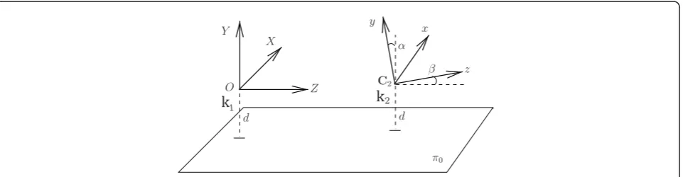
For the above-mentioned reasons, intermediate pro-cessing of the instantaneous homography is necessary. This is achieved in this study by means of a linear esti-mation process based on Kalman filtering. Let us first inspect the analytical expression of the homography between two consecutive instants. Figure 3. illustrates the situation of a vehicle with an on-board camera
moving on a flat road plane, π0 = (nT, d)T, wheren=
(0, 1, 0)Tanddis the distance between the camera and the ground plane. The coordinate system of the camera at time k1 is adopted as the world coordinate system,
where Z-axis indicates the driving direction. At timek2
the camera has moved to positionC2, and rotation Rx (a) might have occurred around theX-axis due to cam-era shaking (adenotes the change in the pitch angle). Additional rotation Ry(b) models variations in the yaw angle (i.e., around theY-axis), which must be consid-ered in the case the vehicle changes lane or takes a curve. From the previous discussion, and assuming a pinhole camera model, the camera projection matrices at timesk1andk2 are, respectively,
P1=K[I|0]
P2=KRx(α)Ry(β)[I| −C2]
(20)
The homographyHrelates the projections,x1 andx2,
of a 3D point, X Î π0, in two different images. Its
expression can be derived from Equation (20). In effect, for the first view it isx1 =P1X =K[I|0] and hence any
point in the ray X= (xT1(K−1)T, ρ)T projects tox1. The
intersection of this ray and the planeπ0 determines the
value of the parameter r: it is π0TX =nTK-1x +dr=
0, and thusr = -nT K- 1x1/d. The projectionx2 of the
pointXinto the second view is
x2=P2X=K Rx(α)Ry(β)[I| −C2]X
=K Rx(α)[Ry(β)| −Ry(β)C2] (xT1(K−1)T, ρ)T
=K Rx(α)[Ry(β)K−1x1+tρ]
=K Rx(α)[Ry(β)−tnT/d]K−1x1
where t = - Ry(b) C2. This vector constitutes the
translation in the direction in which the vehicle is head-ing and is thus given byt= (0, 0, 1)Tv/fr, wherevis the velocity of the vehicle andfris the frame rate. From the above equations, the expression of the homography of
k
k
the planeπ0 betweenk1andk2 is derived:
H=K Rx(α) [Ry(β)−tnT/d]K−1 (21)
At each timekwe have a noisy approximation of the homographyHof the road plane between the previous and the current instant. However, the evolution ofHin temporal domain is assumed to be smooth due to the intrinsic constraints in vehicle dynamics, therefore better estimates can be obtained by filtering noisy measure-ments in time. Temporally filtered estimates of the homography are obtained by modeling H with a zero-order Kalman filter whose state vector is composed of the elementsHijof the homography matrix. The design of the filter is summarized as follows:
xTk ={Hij, 1≤i, j≤3}
xk=xk−1+wk
zTk ={Hijk, 1≤i, j≤3}
zk=xk+vk
The process and measurement noise,wk and vk, are assumed to be given by independent Gaussian distribu-tions, p(w) ~ N(0,Q) and p(v) ~ N(0,R). Observe that the measurement vector is composed of the elements of the instantaneous homography matrix,H k, computed from image correspondences. As stated above, measure-ments are expected to be prone to error due to the usually small set of correspondences available, hence the measurement error should be tuned to be larger than the process noise (in the proposed configuration it isQ = 10-6,R= 10-3).
The designed filter provides corrected estimates for the homography at timek, Hˆk, built from the posterior
estimate of the filter state, xˆk. Most importantly, this
measure can be used as a prediction for the homogra-phy in the next time point. This prediction provides an effective reference to evaluate whether or not the com-puted instantaneous measurement may be erroneous. Indeed, at the current time k, we can compare the instantaneous homographyHkto the prediction made in the previous time instant Hˆk−1: if Hk is close to the expected value Hˆk−1 then the filter equations will be conveniently updated; in contrast, if the matrices are significantly different, then it is natural to think that noisy correspondences were involved in the calculation ofHk.
The distance between matrices is measured according to the norm of the matrix of differences. Specifically, the norm induced by the 2-norm of a Euclidean space is used. This is obtained by performing singular value decomposition (SVD) of the matrix and retaining its lar-gest singular value [38]. The incoming matrices are
accepted and introduced into the Kalman filtering fra-mework only if ||Hk− ˆHk−1|| < t
a. Otherwise, the
measured homography is deemed to be unreliable and the predicted homography is used. The threshold ta modulates the maximum acceptable distance to the pre-dicted matrix, which depends on the kinematic restric-tions of the platform in which the camera is mounted.
In the case of highways, vehicle dynamics are bounded by the maximum speed, the maximum turning angle (i. e., yaw angle, b) and the maximum variation in the pitch angle, a, for a given frame rate. The maximum velocity is considered to be v= 120 km/h (33.3 m/s), as enforced by most nation governments. Additionally, a maximum pitch angle variation ofa=±5° is considered, and an upper bound of b=±3° is inferred for the turn-ing angle accordturn-ing to the standard road geometry design rules. Taking into account these bounds, and assuming an image processing rate of at least 1 fps, the threshold is experimentally found to beta= 60.
5.2.2 Motion-based likelihood model
Once a time-filtered estimate of the homography Hˆk is
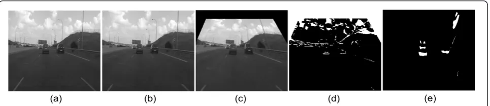
available, reliable image alignment can be performed. Image alignment allows for the location of regions of the image likely featuring motion (and therefore likely containing vehicles). The previous image is aligned with the current image by warping it with Hˆk. Image
align-ment is exemplified in Figure 4. In the upper row, the snapshots of a sequence at times k- 1 and k are dis-played. In Figure 4.c, the image in Figure 4.a warped with Hˆk is shown. Observe that this is very similar in
the road region to the actual image at time k(Figure 4. b).
As suggested in the overview of Section 5.2, the rea-son for image alignment is that all elements in the road plane (except for the points of the vehicle that belong to this plane) are static, and thus their actual position matches that projected by the homography. In contrast, vehicles are moving, hence their positions in the road plane at time ksignificantly differ from those projected by the homography, which assumes they are static. Therefore, the differences between the image at timek and the image at time k - 1 warped with Hˆk shall be
plane) and thus random regions of strong differences arise in the background, which will be considered clutter.
The pixel-wise difference between the current image and the previous image warped provides information on the likelihood of the current object state candidate,si,k. Analogously to the appearance-based likelihood model-ing, the region around the vehicle position indicated by si,k will be evaluated in order to derive its likelihood. Also, to preserve the duality with the appearance-based analysis, the processing is shifted to the rectified domain using the transformation T defined in Section 2. The resulting image, denoted Dr, is illustrated in Figure 4.e for the previous example. In particular, the likelihood of belonging to a region of motion is maximum inxmax=
argmax(Dr (x)), hence a map of probabilities that the pixel xbelongs to a moving region, denotedp(m|x), can be inferred for the whole image asp(m|x) =Dr(x)/Dr (xmax).
From the above discussion, observe that the regions of strong differences are between the current vehicle posi-tion and the posiposi-tion that it would occupy if it were sta-tic (which is always closer to the camera). Therefore, as opposed to the appearance-based modeling (Section 5.1.2), we expect that in the neighborhood below the current vehicle position,si,k, pixels have high likelihood values p(m | x), whereas the neighborhood above x should involve small or null probabilities of motion. Hence, the likelihood of the current vehicle statesi,k regarding the motion analysis is defined as
pm(zi,k|si,k) = 1 (w+ 1)h
⎛
⎝
x∈Ra
(1−p(m|x)) + x∈Rb
p(m|x)
⎞ ⎠
where the regionsRaandRbare those defined in Sec-tion 5.1.2, and the subscriptmin the probability denotes that it refers to motion observation. The likelihood result obtained from the motion-based analysis is finally combined with that achieved after appearance-based
analysis. The joint likelihood of a candidate statesi,kis simply defined as the arithmetic mean of likelihoods:
p(zi,k|si,k) = 1
2(pa(zi,k|si,k) +pm(zi,k|si,k)) (22)
Note that, although the product of likelihoods could have been used instead, the mean is preferred in order to avoid that the calculation be biased by likelihood values that are too small.
6 Vehicle detection
Up to this point, the method for vehicle tracking has been explained. However, in normal driving situations it is natural that vehicles come in and out of the field of view of the camera throughout the sequence of images. While management of outgoing vehicles is fairly straightforward (the track simply exceeds the limits of the image), a method for incoming vehicles must be designed. The method proposed in this study follows a two-step approach. In the first stage, hypotheses for vehicle positions are made using the results of appear-ance-based classification explained in Section 5.1. In the second, they are verified according to the analysis of a set of features in their associated regions in the original domain.
6.1 Hypothesis generation
Exhaustive search of a certain pattern in the entire image is too time-consuming for applications requiring real-time operation. Hence, it is common to perform some kind of fast pre-processing that restricts the search areas. In this case, we exploit the information extracted from the construction of likelihood models for tracking and use it to generate a set of candidate regions that will be further analyzed. In particular, two types of inputs could be used that correspond to the appear-ance-based analysis in Section 5.1 and the motion-based analysis in Section 5.2. As referred to in the correspond-ing section, the latter usually involves noise due to
Figure 4Example of image alignment. Image(a)and(b)correspond to timesk -1 andk, respectively, of the video sequence;(c)is the image atk -1 warped withHˆk;(d)is the difference between aligned images, i.e.,(b)and(c); and(e)is the corresponding image of
background structures, thus appearance-based informa-tion is more suitable for hypothesis generainforma-tion.
Specifically, based on the appearance analysis, for each pixel the probability that it belongs to a vehicle,p(XV | zx) is available. We expect that if there is a new vehicle appearing in the image, a compact zone of high prob-abilities must be observed in the surrounding of its posi-tion. Therefore, in order to localize new vehicles, a binary mapBmis created containing the pixels in which the probability of the vehicle class is larger than that of the other classes,p(XV|zx)> p(Xi|zx),iÎ P,L,U. For example, the binary map obtained for the image in Fig-ure 5.b is shown in FigFig-ure 5.c. Connected component analysis is performed over Bm to extract the regions with a high probability of belonging to vehicles. Result-ing regions are filtered accordResult-ing to a minimum area criterion in order to remove noise.
Naturally, regions corresponding to the tracked vehi-cles should exist inBm. Besides, if there is an additional region inBmthis is regarded as a potential new vehicle in the image and it is further analyzed in the hypothesis verification stage. In particular, in the example in Figure 5.c three regions are obtained: the upper two regions correspond to existing vehicles, labeled 1 and 2, while the small region in the lower left corner constitutes a potential new vehicle (in this case it is actually a vehicle, as can be observed in Figure 5.a). Since only the lower part of the vehicles is reliable in the rectified domain, candidates are characterized by their position and width. As potential vehicles are verified according to their appearance in the original image, their position and width in this domain are computed by means of the inverse transformation T-1. Finally, a 1:1 aspect ratio is initially assumed for the vehicle so that a bounding box Rhcan be hypothesized for vehicle verification.
6.2 Hypothesis verification
Vehicle verification is based on a supervised classifica-tion stage based on SVM. A database of vehicle rear images is generated for the training of the classifier as will be explained in Section 6.2.2. Most importantly the
database separates images according to the region in which the vehicle is found (close/middle range in the front, close/middle range in the left, close/middle range in the right, and far range). Indeed, the view of the vehi-cle rear changes in these areas and thus affects its intrinsic features. This is taken into account in the design of the feature description, which adapts to the particularities of the different areas. Besides, a different classifier is trained for each of them using the corre-sponding subsets of images in the database.
As for the feature description, a new descriptor is proposed based on two characteristics that are inher-ent to the vehicles: high edge continher-ent and symmetry. Indeed, the method automatically adapts the area for feature extraction according to a vertical symmetry-based local window refinement. This allows for the correction of position offsets in the hypothesis genera-tion stage and for the adaptagenera-tion to the vehicle rear contour. Regarding the feature extraction within the refined region, a new descriptor that exploits the inherently rectangular structures of the vehicle rear is designed. The descriptor, called CR-HOG, is based on the analysis of HOG in concentric rectangles around the center of symmetry.
6.2.1 CR-HOG feature extraction
HOGs evaluate local histograms of image gradient orientations in a dense grid. The underlying idea is that the local appearance and shape of the objects can often be well characterized by the distribution of the local edge directions, even if the corresponding edge positions are not accurately known.
This idea is implemented by dividing the image into small regions called cells. Then, for each cell, a histo-gram of the gradient orientations over the pixels is extracted. The original HOG technique, proposed by Dalal and Triggs [12], presents two different kinds of configurations, called Rectangular HOG (R-HOG) and circular HOG (C-HOG), depending on the geometry of the cells used. Specifically, the former involves a grid of rectangular spatial cells and the latter uses cells parti-tioned in a log-polar fashion.
Figure 5Example of generation of a new vehicle hypothesis. The sequence of images is the following:(a)original image,(b)rectified image,(c)binary mapBmcorresponding to appearance analysis in (b): pixels in white indicate potential location of vehicles. In the example, the
As stated, in this study we present a new configura-tion for the cells that better adapts the characteristics of the vehicles. Indeed, the rear of the vehicles presents an inherently rectangular structure: not only is the outer contour of the vehicle rear quasi-rectangular, but the inner structures such as the license plate and the rear window are also rectangular. Hence, we naturally define a new configuration of HOG composed of concentric rectangular cells as shown in Figure 6.a. This structure will be referred to as CR-HOG (for concentric rectan-gle-based HOG). The layout of the CR-HOG has five parameters: the number of concentric rectangles b, the number of orientation binsn, the center csof the win-dow, its heighths, and its widthws.
In practice, the hypothesized region for vehicle verifi-cation,Rh, may not perfectly fit the actual bounding box of the vehicle in terms of size and alignment. Specifi-cally, it is often the case that the vehicle is not perfectly centered in Rh, especially on the horizontal axis. There-fore, direct application of CR-HOG (or of standard HOG) over Rh will possibly result in degraded perfor-mance. Instead, we refine the region likely containing the vehicle through the analysis of vertical symmetry in the intensity of the region. In particular, the subregion within Rhgiving the maximum degree of vertical sym-metry is kept for HOG computing. Vertical symsym-metry is calculated using the method in [39]. As a result, we obtain the axis of vertical symmetry,xsand the width of the region that maximizes the symmetry measure, ws. The height hs of the window for HOG application is taken as that of Rhand its center is thus given by cs= (xs,hs/2).
Figure 6.b illustrates the window adaptation approach based on symmetry analysis. Observe that the refined vertical side limits (colored in red) fit much better the bounding edges of the vehicle rears. In practice, the area for calculation of CR-HOG is extended by a 10% so that the outer edges of the vehicle are also accounted for in the descriptor.
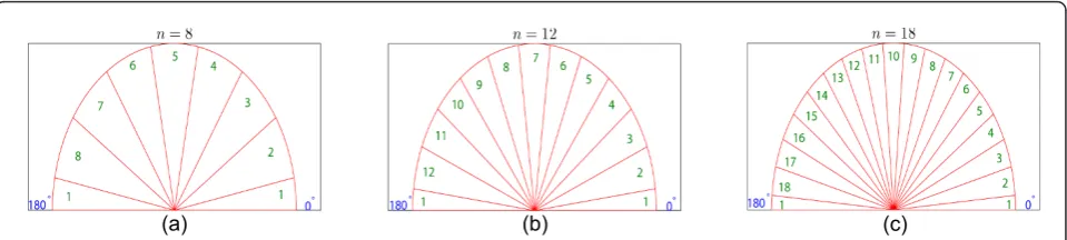
The steps for the calculation of CR-HOG on the refined window are the following. First, the gradient magnitude and orientation are computed at each point of the window using a standard operator (Sobel 3 × 3 masks are used in our implementation). Then, in order to create a histogram of orientations, a number of orien-tation bins is defined and each pixel votes for the bin that contains its corresponding angle. The votes are weighted by the magnitude of the gradient at that point. Three possible configurations have been considered involvingn= 8, 12, and 18 bins evenly spaced over [0, 180), as illustrated in Figure 7.
The bins have been shifted so that the vertical and horizontal orientations, which are very frequent in the rear of vehicles, are in the middle of their respective bins. This way, small fluctuations around 0° and 90° will not affect the descriptor. The histogram of each cell is finally normalized by the area of the cell so that histo-grams of different cells are in the same order of magni-tude. The CR-HOG descriptor is composed of the normalized histogram of orientations of all the cells. The optimal configuration of the number of orientation bins, n, and the number of cells,b, is discussed in Sec-tion 7 for each region of the image.
6.2.2 Classification stage
The CR-HOG descriptors are introduced in a Support Vector Machine-based classifier. A new database con-taining 4,000 positive vehicle images and 4,000 negative vehicle images is used to train and test the classifier (this can be accessed in the Internet [40]). The core of the database is composed of images from our own col-lection. Additionally, images have also been extracted from the Caltech [41,42] and the TU Graz-02 [43,44] databases and included in the data set. The joint data-base consists of images of resolution 64 ×64 acquired from a vehicle-mounted forward-looking camera. Each image provides a view of the rear of a single vehicle. Some images contain the vehicle completely while others have been drawn to contain it only partially (all
images contain at least 50% of the vehicle rear) in order to simulate putative results of the hypothesis generator.
Images involve many different viewpoints of the vehi-cle rear corresponding to vehivehi-cles in different locations relative to the vehicle in which the camera is mounted. Specifically, the space is divided into four main regions: close/middle range in the front, close/middle range in the left, close/middle range in the right, and far range. The database contains 1,000 images of each of these views. A set of 4,000 images not containing vehicles have also been used to train and test the classifier. The images are selected in such a way that the variability in terms of vehicle appearance, pose, and acquisition con-ditions (e.g., weather concon-ditions, lighting) is maximized. A classifier based on SVM using linear basis functions is used for each of the four image regions.
7 Experiments and discussion
Experiments regarding the proposed method have been performed twofold. On the one hand, the performance of the novel CR-HOG based approach for vehicle detec-tion is tested on the database referred to in Secdetec-tion 6.2.2. On the other hand, experiments have been carried out in the complete system integrating vehicle detection and tracking over a wide variety of video sequences.
7.1 Experiments on vehicle detection
The SVM-based classifier for vehicle detection explained in Section 6 has been trained and tested in Matlab using the Bioinformatics Toolbox. The method involves two design parameters, namely the number of orientation bins in the histogram, n, and the number of cells, b.
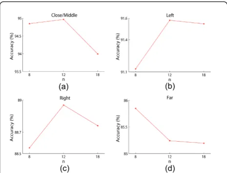
Experiments have been performed on the database for values n= 8, 12, 18 and b = 2, 3, 4. A cross-validation procedure is used to test the method. Specifically, 50% of the images are randomly selected for the training set and the remaining 50% are used for the testing set. This process is repeated 5 times and the average is computed. The accuracy or correctly classified rate of samples as a function of these parameters is provided in Table 1 for each of the four regions. These results are graphi-cally represented in Figures 8. and 9. to facilitate their interpretation. In particular, Figure 8. shows the accu-racy results as a function of the number of cells, b, by averaging onn, for each area of the image. Analogously, Figure 9. illustrates the average accuracy results as a function of the number of orientation bins,n.
As a first conclusion of the experiments we can infer that the accuracy decreases forb = 4 in all the areas of the image. As for the number of orientation bins, a dif-ferent behavior is observed for the frontal and the sides views. Specifically, for the central close/middle and far ranges similar results are obtained forn= 8 and n= 12, while the performance decreases notably for n= 18. On the contrary, for the left and right areas a significant accuracy increase is observed from n = 8 ton = 12; a further increase ton= 18 does not bring an additional gain. This contrast is indeed reasonable since, from a completely orthogonal viewpoint, the edges of a vehicle are fairly invariant and mostly vertical and horizontal; conversely, in the side views the upright edges corre-sponding to the back window and its contour (especially the furthest from the image center) tend to divert from verticality. Consequently, more variability is found in
Figure 7Possible configurations of CR-HOG regarding the number of orientation bins. The range of gradient orientation angles [0-180) is divided in uniformly spaced sectors. Pixels with gradient orientations inside each sector accumulate to the corresponding bin of the histogram proportionally to the magnitude of their gradient. Configurations with(a)8,(b)12, and(c)18 bins are considered.
Table 1 Classification accuracy rates of CR- HOG
Close/Middle Left Right Far
b= 2 b= 3 b= 4 b= 2 b= 3 b= 4 b= 2 b= 3 b= 4 b= 2 b= 3 b= 4
n= 8 94,88 94,98 94,68 91,04 91,18 91,16 88,58 89,14 87,94 85,92 85,86 85,76
n= 12 94,96 94,80 95,14 91,46 91,82 91,46 89,28 89,42 88,16 85,32 85,24 85,16
the gradient orientation map, and therefore more bins are necessary to capture fine-detail.
A good trade-off between complexity and performance is achieved by selecting (b,n) = (2, 8) for the close/mid-dle and far ranges, and (b,n) = (3, 12) for the left and right views. This involves respective detection accuracies of 94.88, 85.92, 91.82, and 89.42%, which results in an average correct detection rate of 90.51%. The rate differ-ence between left and right views is due to the particu-larities of the traffic participants in the right lane, which usually includes slow vehicles (buses, trucks, vans, etc.). These involve a great appearance variety and hence make classification much more challenging. Naturally,
the worst classification rate is obtained for the furthest vehicles, in which the edge-details are degraded. The results are improved to an overall accuracy of 92.77% when using a Gaussian radial basis function kernel (instead of the linear kernel), with respective correct detection rates of 96.14, 89.92, 94.14, and 90.86% for the different areas. However, the proposed method continu-ously generates hypotheses for the potential vehicles. Hence, even if a vehicle is not detected in a given frame, it is usually detected in the following frames. Therefore, the small latency incurred by the linear kernel-based classification is usually negligible and it is not necessary to use more complex kernels.
7.2 Experiments on vehicle tracking
In regard to vehicle tracking, the designed method has been tested on a wide variety of sequences recorded on Madrid, Brussels, and Turin. These sequences, which were acquired in several sessions with different driving conditions (i.e., illumination conditions, weather, pavement color, traffic density, etc.), amount to 22:38 min. Test sequences were acquired from a forward-looking digital video camera installed near the rear mirror of a vehicle driven in high-ways. The method is able to operate near real-time at 10 fps on average over an Intel(R) Core(TM) i5 processor run-ning at 2.67 GHz. Implementation is done in C++.
The above-mentioned test sequences are used to com-pare the performance of the proposed tracking method with the two methods most widely used in the literature. Namely, those involve independent tracking of multiple objects with a Kalman filter assigned to each object (which will be referred to as KF-based tracking), or joint tracking using PF based on importance sampling
Figure 8Classification accuracy as a function of the number of cells,b. The results are broken down for images corresponding to(a)close/ middle,(b)left,(c)right and(d)far views.
Figure 9Classification accuracy as a function of the number of orientation bins,n. The results are broken down by zones:(a)
(shortly, SIS-based tracking). For the implementation of KF-based tracking, appearance-based region labeling through connected-component analysis is used as in Section 6.1 to locate vehicles in every frame, and tracks are formed temporally by matching the regions accord-ing to a minimum distance criterion. As for SIS-based tracking, a sequential resampling scheme is used (see details of the algorithm in [21]). Additionally, the motion model used for SIS-based tracking is exactly that designed for the proposed method, while KF-based tracking uses the same dynamic model for independent motion of vehicles, but cannot accommodate any inter-action model. Other parameters of the dynamic model are wl = 90 and ds = 96. Regarding the observation model, the dimensions of the local windows RaandRb are set to w =h= 10. Also, the standard deviation of the proposal density is optimally calculated for the pro-posed method and for SIS-based tracking assq = (2, 3) and sq = (5, 8), respectively. Finally, the same number of samplesN= 250 is used for both methods.
To compare methods, the number of tracking failures incurred by each of the methods on the same test sequences is counted. A tracking failure occurs when the tracker fails to provide continuous and coherent measures for a given vehicle inside the region of interest (ROI). The ROI is defined to be the scope of the IPM, which usually comprises the own and the two adjacent lanes, and extends longitudinally up to a distancedfthat depends on the camera calibration. Comparative results are displayed in Table 2. As expected, the proposed method largely outperforms the others in terms of tracking failures in the test sequences. Naturally, KF-based tracking delivers the highest error rate as it is unable to handle situations in which vehicles interact. Notably, SIS-based tracking also outputs a significant number of errors, since the number of particles is rela-tively small and these fail to correctly sample the space when the number of vehicles grows.
7.3 Analysis of computational complexity
The computational cost of the different processing blocks of the method is summarized in Table 3. As can be observed, the appearance analysis is naturally the most costly module (44% of the processing time per frame) as it constitutes the core for the definition of the observation model and is in the basis of the hypotheses generation for vehicle detection. Most remarkably, the vehicle tracking algorithm consumes only 23.98% of the processing time thanks to the efficient MCMC sampling. Indeed, compared to traditional particle filtering based on importance sampling, the processing load of sam-pling is largely lightened. In MCMC, for a given number of objectsM, a Markov chain of lengthC·Mis created, in which the state of each object changes on averageC times (in each step of the chain only one random object is moved). Hence, samples generated from the chain may comprise a number of possible object state combi-nations at the order of CM. In contrast, in SIS-based sampling, particles are independently generated and each corresponds to a possible state combination, there-foreCMparticles are necessary to obtain the same num-ber of combinations as in MCMC. Consequently, since each particle involves evaluation of the posterior density in (11) both for MCMC and SIS, the complexity of the proposed sampling algorithm isΩ (C · M) whereas that of SIS-based sampling is Ω(CM). The Big Omega Ωis used here to denote the lower bound, since a number of lighter additional operations are also involved in sam-pling besides posterior density evaluation. In other words, the complexity of the sampling algorithm grows linearly in the proposed method, while the traditional SIS grows exponentially. Complexity comparison between methods is summarized in Table 4.
The real-time operation requirement constrains the processing time available for particle propagation and thus the efficiency of the sampling is crucial to the per-formance of the method. As shown in Table 5, if we limit the number of particles toN= 250, for which near real-time operation is attained (approximately 10 fps), SIS-based tracking delivers 31 tracking failures in the test sequences described above, whereas with the same computational resources the proposed method outputs only 9 failures. Even if the number of particles for SIS-based tracking is increased to N = 1000, the tracking failures still outnumber largely those of the proposed method, while the average frame rate plummets far from real-time. As a matter of fact, if we consider a Table 2 Summary of tracking results
Method Tracking failures
Number of frames
Number of vehicles
KF-based Tracking
36
SIS-based Tracking
31 33454 120
Proposed Method
9
Table 3 Average processing time of the proposed algorithm per block
Appearance analysis Motion analysis Vehicle detection Sampling Total
Processing time (ms) 44.33 9.15 19.54 23.04 96.06