R E S E A R C H
Open Access
Performance analysis and improvement of dither
modulation under the composite attacks
Xinshan Zhu
1,2*and Jie Ding
1,3Abstract
The first goal of this article is to analyze the performance of dither modulation (DM) against the composite attacks including valumetric scaling, additive noise and constant change. The analyzes are developed under the
assumptions that the host vector and noise vector are mutually independent and both of them have
independently and identically distributed components. We derive the general expressions of the probability density functions of several concerned signals and the decoding error probability. The specific theoretical results are provided for the case of generalized Gaussian host and noise. Based on the analyzes, the performance of DM is predicted for different scenarios with a high degree of accuracy and evaluated for different distribution models of host and noise signals. Numerical simulations confirm the validity of the given theoretical analyzes. Then, we address to improve the robustness of DM against valumetric scaling plus constant change. The normalized dither modulation (NDM) is presented, which works by constructing a gain-invariant vector with zero mean for
quantization. Performance analysis shows that NDM is theoretically invariant to valumetric scaling and constant change and achieves similar performance to DM in other aspects. The performance of NDM is further improved by weighting the quantization errors. Experiments on real images also show the advantage of NDM over DM subject to amplitude scaling and constant change.
Keywords:digital watermarking, quantization index modulation, composite attacks, valumetric scaling, constant change
1 Introduction
In the past decade, much attention has been paid to the quantization-based watermarking for canceling the host signal interference. One of the most important methods proposed so far is quantization index modulation (QIM) [1]. The basic QIM algorithm includes a number of var-iants, i.e., dither modulation (DM), distortion compen-sated dither modulation (DC-DM) (also known as scalar Costa scheme (SCS) [2]) and spread transform dither modulation (STDM) [1]. The theoretical performance of QIM methods is a key issue and has received consider-able attention.
Initially, the Gaussian channel is often used in the analyzes and the performance of QIM methods has been extensively investigated in this case. A relatively crude approximation to the decoding error probability
of QIM was given in [1] for the additive white Gaussian noise (AWGN) attacks. The performance of SCS was completely analyzed by Eggers et al. [2] under the AWGN attacks. In [3], the performance of scalar DC-QIM against AWGN was theoretically evaluated from the detection viewpoint. Recently, a new logarithmic QIM (LQIM) was presented in [4] and its performance was analyzed in the presence of AWGN. It has been pointed out in [5] that the performance of QIM meth-ods may be overstated under Gaussian channels. In the second phase, a deeper analysis is done for QIM taking into account a much wider variety of attacks. The care-ful performance analyzes were presented by Pérez-Gon-zàlez et al. [5] for a large class of QIM methods in the cases of uniform and Gaussian noise. Bartolini et al. [6] concentrated on analyzing the performance of STDM in the presence of two important classes of non additive attacks, the gain attack plus noise addition and the quantization attack. In [7], the authors proposed an improved DM scheme to resist linear-time-invariant * Correspondence: [email protected]
1
School of Information Engineering, Yangzhou University, Yangzhou 225009, China
Full list of author information is available at the end of the article
filtering and provided a thorough analysis of it. We notice that most of previous analyzes make use of the Gaussian host assumption and even neglect the statisti-cal properties of the host signal.
The conventional QIM has a serious drawback, i.e., the weakness against valumetric scaling. Spherical codes were utilized to cope with this problem in [8]. However, watermark embedding and recovery get very compli-cated [9]. Oostveen et al. [10] proposed to choose the adaptive quantization step size to be proportional to a local average of the host signal samples. Despite its robustness against valumetric scaling, the method pre-sents a nonzero probability of error even for null distor-tions and becomes more sensitive to constant change. Rational dithered modulation (RDM) was developed in [9] using a gain-invariant adaptive quantization step size at both embedder and decoder. The RDM achieves invariance to valumetric scaling, but is still sensitive to constant change. Li and Cox [11] applied the modified Watson’s perceptual model to provide resistance to valumetric scaling for QIM watermarking. The modifi-cation to Watson’s model results in the degradation in quality and performance loss with respect to constant change.
The first objective of this article is to analyze the per-formance of DM against composite attacks, which is lacking in the literature. Obviously, in watermarking applications, it is more often that the watermark under-goes multiple attacks. Specifically, the combination of valumetric scaling, additive noise and constant change will be considered. On the other hand, most of previous analyzes are restricted to the Gaussian noise channel, even sometime regardless of the distribution of the host signal, which we will try to overcome. The generalized Gaussian distribution (GGD) is adopted to model both the host signal and the noise signal in our analysis. Since the GGD is a parametric family of distributions, we will observe how the choice of distribution model affects the performance of DM. Next, the weakness of DM is concerned. DM itself is largely vulnerable to valumetric scaling as well as constant change. Several existing improved DM schemes achieve the robustness against valumetric scaling, but becomes more sensitive to constant change. We will present the normalized DM (NDM) considering both of them. Under the light of the performance analyzes done for DM in this article, we show that NDM approaches the performance of DM, with the great advantage of insensitivity to valumetric scaling and constant change.
The rest of this article is organized as follows. Section 2 reviews the original DM and describes the problems to be solved. Next, Section 3 accurately derives the gen-eral PDF models for sevgen-eral relevant signals. In Section
4, the performance of DM under the composite attacks is mathematically analyzed by the derived PDFs. The decoding error probability is given in closed form and the theoretical results are confirmed by numerical simu-lations. Then, in Section 5, the NDM method is pre-sented and its performance is theoretically evaluated. Section 6 provides a useful strategy to improve the per-formance of NDM. In Section 7, a series of tests on real data are done to verify the validity of analytical deriva-tions and evaluate the presented approaches. Finally, Section 8 concludes.
Notation: In the remainder of this article, we use bold-face lower-case letters to denote column vectors, e.g.,x, and scalar variables are denoted by italicized lower-case letters, e.g., x. The probability distribution function (PDF) of a random variable (r.v.)xis denoted bypX(x),
whereas if x is discrete its probability mass function (PMF) is designated by PX(x). We write x ~ pX(x) to
indicate that a r.v. x is distributed as pX(x). pX|Y(x|y)
means the conditional probability ofx giveny. And the subscripts of the distribution functions will be dropped wherever it is clear the random variables they refer to. Finally, the mathematical expectation and standard deviation are respectively represented byμxand sxfor a
r.v.x.
2 Review of DM and problem
We will concentrate our attention on DM in this study. The uncoded binary DM can be summarized as follows.
Letx ÎℝN be a host signal vector in which we wish to embed the watermark message m. First, the message mis represented by a vector bwithNRm binary
antipo-dal components, i.e.,bj= ± 1, j= 1, ..., NRm, whereRm
denotes the bit rate. The host signal x is then decom-posed into NRm subvectors (blocks) of length L =⌊1/ Rm⌋, denoted byx1,. . .,xNRm. In the binary DM, twoL
-dimensional uniform quantizers Q-1(·) and Q+1(·) are
constructed, whose centroids are given by the lattices and Λ-1 = 2ΔℤL+d and Λ+1= 2ΔℤL +d +Δawithd ÎℝL
a key-dependent dithering vector and a= (1, ..., 1)
T
. Each message bit bj is hidden by usingQbj(·)on xj,
resulting in the watermarked signalyÎℝNas
yj=Qbj(xj), j= 1,. . .,NRm. (1)
The watermark detector receives a distorted, water-marked signal, z, and decodes a messagemˆ using the minimal distance decoder
bj= arg min
−1,1Qbj(zj)−zj, j= 1,. . .,NRm, (2) where ||·|| stands for Euclidean (i.e.,ℓ2) norm.
well known that quantization-based watermarking is vulnerable to valumetric scaling attack. While the vector at the input of the decoder is scaled byrj, i.e.,zj=rjyj,
the quantization bins at the decoder are not scaled accordingly, thus producing a mismatch between embedder and decoder that dramatically affects perfor-mance. Also, the original DM is not robust to constant change distortion, i.e., zj =yj+ cja with cja constant
value. No decoding error is made for |cj|<Δ/2, however,
the bit error rate (BER) is equal to 1 for Δ/2<|cj|<3Δ/
2. In this study, the two attacks are considered together with additive noisevj, yielding the attacked signal as
zj=ρjyj+νj+cja. (3)
We will analyze the performance of DM in the case of (3), and present an improved DM resisting both valu-metric scaling and constant change. In the subsequent analysis,x,y,zandνare all regarded as random vectors. And we assume that bothx and vhave independently and identically distributed (i.i.d.) components and vis independent from y. Since the mean value of additive noiseνjcan be counted by the third term in the
right-hand side of (3), it is reasonable to assume thatμv= 0.
3 PDF models
Define the extracted vectorr,rQb(z)−z. Obviously,
a crucial aspect when performing a rigorous analysis lies in computing the PDF ofr. Let us begin with the issue.
3.1 PDF model of the watermarked signal
We use a lower-case letter to indicate any element of the vector denoted by the boldface one. The previously used index jis dropped for no specific values (or sub-vectors) are concerned. Givenx ~ pX(x), from the
rela-tion (1), the PDF of the watermarked signal y conditioned on a transmitted symbolbis written as
pY(y|b) = ∞
k=−∞
δ(y−yk) yk+
yk−
pX(x)dx, (4)
where the variableykis defined asyk= 2kΔ+ (b + 1)
Δ/2 +dandδ(·) denotes the delta function.
A few observations are in order about the PDF of y. First, for different dither value d, the PDFpY(y|b) is
dif-ferent. That means each element of y obeys different distributions by randomly selectingdduring embedding. However, due to the factPY(yk+2Δ|b) =PY(yk+1|b) exists,
it is sufficient for us to consider the cased Î [-Δ,Δ). Further, if the PDF pX(x) is symmetric, i.e., pX(x) =pX
(-x), from (4), the PDFpY(y) satisfies pY(y|b=-1) =pY
(-y|b= 1) for the case ofd=-Δ/2 andpY(y|b) =pY(-y|b)
for the case of d = 0. The former indicates that the PDFs pY(y|b=-1) andpY(y|b = 1) are mirrors of each
other and the latter indicates that the PDFpY(y) is even.
These two properties ofpY(y) are exhibited in Figure 1.
3.2 PDF model of the attacked signal
Taking the Equation (3) into account and using the fact
that for any ρ >0pρY(y) =ρ1pY
y
ρ
holds, the
condi-tional PDF of zgiven the transmitted symbolb can be obtained by convolution [12]
pZ(z|b) = ∞
k=−∞
PY(yk|b)pv(z−ρyk−c), (5)
where the convolution follows from the independence betweenyandν. Observing (5), if the effect of different d on PY(y) is ignored (this generally holds when the
embedding distortion is acceptable), the PDF pZ(z|b)
withd≠0 can be approximately viewed as the translate of pZ(z|b) withd = 0, that is,pZ(z+rd|b, d≠0) ≈ pZ
(z|b,d= 0).
−2000 −1500 −1000 −500 0 500 1000 1500 2000 0.02
0.04 0.06 0.08 0.1 0.12 0.14
y pY
(y|b)
Gaussian host: Δ=50, d=−25
b=−1 b=+1
(a)
−2000 −1500 −1000 −500 0 500 1000 1500 2000 0.02
0.04 0.06 0.08 0.1 0.12 0.14
y pY
(y|b=
−
1)
Gaussian host: Δ=50, d=0
(b)
Figure 1The PDF curves ofyfor zero-mean Gaussian host data with variance 2552:(a)
Moreover, when bothxandν are distributed symme-trically around the origin, we have the mirror property pZ(z + 2c|b= -1) = pZ(-z|b= 1) for the case d =-Δ/2,
and the symmetric property pZ(z+ 2c|b) =pZ(-z|b) for
the cased= 0.
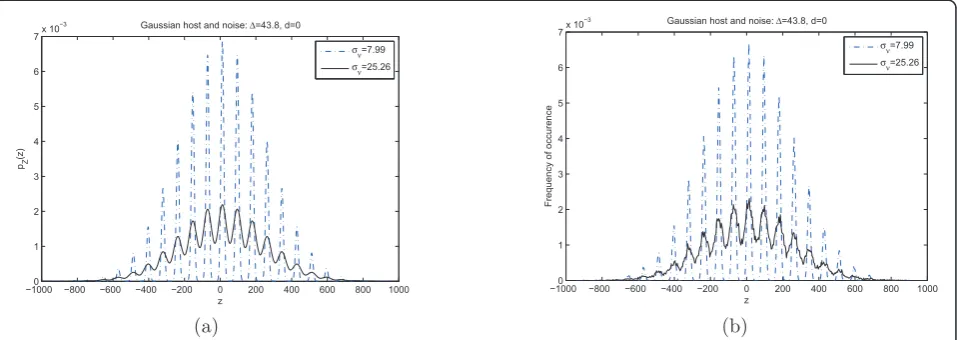
Figure 2a depicts qualitatively the PDFs of zfor zero-mean Gaussian host data with variance 2552 and zero-mean Gaussian noise. It can be seen that there is a bell curve present around each discrete value ofy due to the existence of Gaussian noise, and the two adjacent ones even overlap for a large noise strength. Meanwhile, the distance between two discrete points of y is scaled by the scaling factor rand pZ(z) is translated by constant
valuec. The corresponding empirical density curves ofz are plotted in Figure 2b. We see that the analytical PDF ofzfits well with empirical observations.
3.3 PDF model of the extracted signal
Recalling the definition of r given previously, it is immediate to write
pR(r|b) = ⎧ ⎨ ⎩
∞
j=−∞
pZ(zj−r|b,d),r∈[−,)
0, else,
where pR(r|b) is the PDF of r conditioned on the
transmitted symbolb, andzjhas the similar definition
withyk. Due to (5), the above equation becomes
pR(r|b) =
j
k
P(yk|b)pv(μjk−r),r∈[−,)
0, else
(6)
withμjk=zj-ryk-c.
Now, let us analyze the properties of pR(r). If ignoring
the effect ofd onPY(y), in view of (6), we derive pR(r
d|b,d ≠0)≈ pR(r|b,d = 0) with =r - 1. This shows
that for the case d≠0 the PDFpR(r|b) can be
approxi-mately obtained by translating pR(r|b, d = 0). Further,
while|| is small enough for neglecting the term d, we have the property pR(r|b, d≠0) ≈ pR(r|b, d= 0). That
is, despite the choice of d,pR(r) approximately remains
unchanged for small ||. Similarly topZ(z), by assuming
the PDFspX(x) andpν(ν) are even, we obtain the mirror
property pR(r -2c|b= 0) = pR(-r|b= 1) for d=−2 and
the symmetric property pR(r -2c|b) =pR(-r|b) for d= 0.
At the same time, for any , we derivepR(r|b, r =1 + ) = pR(r|b, r = 1-ε) for d = 0 andpR(r|b = 0,r = 1 +
ε) = pR(r|b = 1, r = 1-ε) for d=−2, where pR(r|b, r)
denotes the conditional PDF ofr given the transmitted symbol b and the scaling factor r. These properties of pR(r) are helpful for us to analyze the performance of
DM.
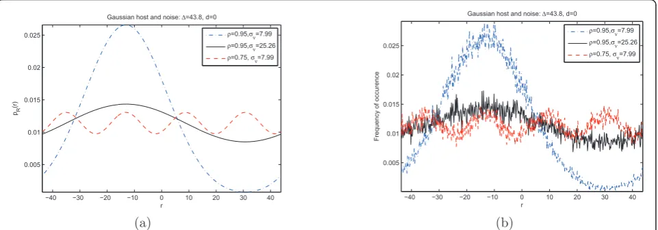
Figure 3 plots the probability density curves ofr and the corresponding empirical ones for zero-mean Gaus-sian host data with variance 2552 and zero-mean Gaus-sian noise. As can be seen, the distribution curve of ris either dilated or compressed by the scale factor r, and the PDFpR(r) withc ≠0 corresponds topR(r) with c=
0 translated by the constant value c. The probability that the values of r are distributed around zero decreases as attacks become strong, which results in the increase of BER. Comparison of Figure 3a, b reveals the analytical PDF of r fits perfectly with its empirical distribution.
4 Performance analysis of DM against the composite attacks
As the previous literatures, the decoding bit error prob-abilityPeis used as the final performance measurement.
−10000 −800 −600 −400 −200 0 200 400 600 800 1000 1
2 3 4 5 6 7x 10
−3
z pZ
(z)
Gaussian host and noise: Δ=43.8, d=0
σν=7.99 σν=25.26
(a)
−10000 −800 −600 −400 −200 0 200 400 600 800 1000 1
2 3 4 5 6 7x 10
−3
z
Frequency of occurence
Gaussian host and noise: Δ=43.8, d=0
σν=7.99 σν=25.26
(b)
Assuming that the symbolb is sent, the bit error prob-ability will be
Pe=P(||r||>||a− |r||||b) (7)
where |r| denotes the vector of absolute values of components of r. Defining s|r|Ta, the above expres-sion is equivalent to
Pe = L
L/2
pS(s|b)ds. (8)
To computePe, we need know the PDFpS(s) ofs. The
exact solution for pS(s) may be achieved by several
means. One of the standard procedures is by performing multifold integral operation as
pS(s|b) = (L−1)
0 . . .
2
0
0
p|R1|(u1|b)p|R2|(u2−u1|b)
...p|RL|
s− L−1
i=1
ui|b
du1du2· · ·duL−1, (9)
wherep|Rj|(rj|b) =pRj(rj|b)+pRj(-rj|b) andpRj(rj) is the
PDF of thejth element ofr. The computation ofpS(s) is
feasible for a small L by (9). However, it becomes impractical as Lincreases. To solve the problem, it is nature to use mathematically tractable approximations. Let us assume that all components of d are equal, so that the vectorrhas i.i.d components. At this point, by the well known central limit theorem (CLT),sthus can be approximated by a Gaussian random variable, whose mean and variance areLμ|r|andLσ|2r|.Using the derived
PDF in (6),μ|r|andσ|2r|are represented as
μ|r|=
j
k
P(yk|b)
−
|u|pν(μjk−u)du (10)
σ2
|r|=
j
k
P(yk|b)
−
u2pν(μjk−u)du−μ2|r|. (11)
Then, the probabilityPeis computed as
Pe≈
√
L(−μ|r|)
σ|r|
−
√
L(/2−μ|r|)
σ|r|
,(12)
whereF(·) stands for the cumulative distribution func-tion (CDF) of the standard Gaussian distribufunc-tion. It should be pointed out the CLT approximation to Peis
only valid for very largeL. In reality, the condition is generally met in order to improve the watermarking robustness.
Now, we can observe several useful properties of Pe
from the previous analysis. When||is small enough, by the property pR(r|b, d≠0) ≈ pR(r|b, d= 0), it is easily
understood that Peapproximately remains unchanged
for different dither value. Therefore, without loss of gen-erality, dis set to 0. Furthermore, for d= 0, if both pX
(x) andpν(ν) are even, using the propertypR(r|b, r= 1
+) =pR(r|b,r= 1-), the same value ofPeis obtained
for the cases ofr = 1-andr = 1 +. As a result, the property ofPealso holds ford≠0 approximately.
4.1 Generalized Gaussian host and noise
Theoretically,Pecan be estimated only if the PDFspX(x)
andpν(ν) are given. For the following analysis we
con-sider a specific case where the host signal and attacking noise are statistically modeled by the GGD. The GGD
−40 −30 −20 −10 0 10 20 30 40
0.005 0.01 0.015 0.02 0.025
r
Gaussian host and noise: Δ=43.8, d=0
pR
(r)
ρ=0.95,σν=7.99 ρ=0.95,σν=25.26 ρ=0.75,σν=7.99
(a)
−40 −30 −20 −10 0 10 20 30 40
0.005 0.01 0.015 0.02 0.025
r
Gaussian host and noise: Δ=43.8, d=0
Frequency of occurence
ρ=0.95,σν=7.99 ρ=0.95,σν=25.26 ρ=0.75,σν=7.99
(b)
model is used because it includes a family of distribu-tions and suitable for many practical applicadistribu-tions. The PDF of the GGD is defined as
p(t) = κβ 2(β−1)e
−|κ(t−μ)|β
, (13)
where κ = 1σ(3β−1)/(β−1), and (u) =0∞tu−1e−tdt is the Gamma function. Thus, the
distribution is completely specified by the meanμ, the standard deviationsand the shape parameter b, and is denoted as GGD(b; μ,s). The CDF of the GGD has the form [13]
(t) = 1
2+sgn(t−μ)
γ(β−1,|κ(t−μ)|β) 2(β−1)
whereγ(u1,u2) = u2
0
tu1−1e−tdtis the lower
incom-plete gamma function, andsgn(·) denotes the sign func-tion, i.e.,
sgn(t) =
1,t≥0 −1, else.
Note that Gaussian and Laplacian distributions are just two special cases of the GGD withb= 2 and b= 1, respectively.
First, the PMFPY(y) is calculated according to the
dis-tribution model ofx. GivenpX(x) ~ GGD(bx;μx,sx) and
the corresponding CDFΨx(x), in view of (4), we
imme-diately write
PY(yk|b) =x(yk+)−x(yk−). (14)
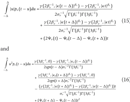
Then, the integration terms in (10) and (11) are derived for the case pν(ν) ~GGD(bν; 0, sν). In appen-dix, we obtain
−
|u|pν(t−u)du=γ(2β−
1
ν ,|κ(t−)|βν)−γ(2βν−1,|κt|βν) 2σ−1
ν
(β−1
ν )(3β−1
ν )
+γ(2β−
1
ν ,|κ(t+)|βν)−γ(2βν−1,|κt|βν) 2σ−1
ν
(β−1
ν )(3β−1
ν ) + (2ν(t)−v(t−)−ν(t+))t
(15)
and
− u2p
ν(t−u)du=γ(3β
−1
ν , 0)−γ(3β−ν1,|κν(t−)|βν)
2sgn(t−)σ−2
ν (3β−1
ν )
+γ(3β
−1
ν ,|κv(t+)|βν)−γ(3βν−1, 0)
2sgn(t+)σν−2(3β−ν1)
−(γ(2βν−1,|κ(t+)|βν)−γ(2β−ν1,|κ(t−)|βν))t σ−1
ν
(β−1
ν )(3β−1
ν ) + (ν(t+)−ν(t−))t2
(16)
Now, the decoding bit-error probability can be esti-mated by computing (10), (11), and (12) with the use of
(14), (15), and (16). Since the calculation ofpY(y) is
rela-tively simple in (4), the above analysis can be easily extended for other host distributions. However, the deri-vation of the integration terms in (10) and (11) might become very complex for the noise ν with other PDFs. Thus, they are computed numerically when needed.
4.2 Simulations on artificial signals
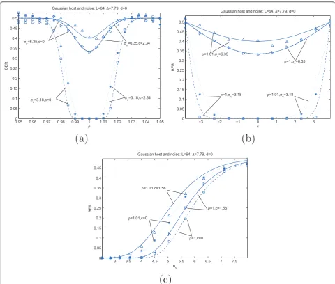
In order to verify the obtained theoretical results, we conduct a set of experiments on artificial signals. A set of 64000 random data, independently drawn from the GGD with zero mean and variance 2552, are used as the host signal. A random message with equiprobable infor-mation bit is embedded using DM with L = 64,Δ = 7.79, and d = 0. The noise signal is also generated according to the zero-mean GGD. We calculated the empirical BER under the composite attacks, and com-pared them to the theoretical values. The obtained results are summarized in Figure 4 for the case of Gaus-sian host and noise.
Figure 4a shows the BER of DM as a function of the scaling factorrwhile fixing the constant valuecand the noise standard deviationsν. As can be seen, DM is defi-nitely very sensitive to the scaling attack. The probability of error is unacceptably high whenrmovies beyond the range [0.98, 1.02]. The existence of noise and constant change causes the increase of BER further. And the effect of constant change becomes relatively distinct for strong noise. The theoretical approximation of BER agrees almost perfectly with the empirical results, parti-cularly in the case of weak attacks. Figure 4a also demonstrates that the BER versus rcurve is symmetric with respect to the pointr = 1. Figure 4b depicts the plots of BER versus the constant valuecwhile fixing the scaling factorrand the noise standard deviationsν. For smallrand sν, the BER of DM starts to grow rapidly as long as the absolute value of capproaches toΔ/2. The effect of c on performance decreases as r and sν increase. The estimated BERs are approximately equal to the empirical ones, but the estimation accuracy gets worse for a large c. At the same time, Figure 4b shows that the BER versusc curve is symmetrical aroundc= 0. Figure 4c plots the BER of DM as a function of the noise standard deviationsνwhile fixing the scaling
fac-tor r and the constant value c. Obviously, the BER increases assνbecomes large. The curve of BER versus
sνseems to be translated due to the effect of valumetric
scaling and constant change distortions. Similar to the previous tests, the theoretical BERs fit the empirical ones very well and the maximal difference between them is lower than 0.02.
attacks for different host PDF shapes controlled by bx.
The results are displayed in Figure 5a. It is remarkable that the performance of DM increases significantly asbx
goes down. For a smallbx, the BER plot becomes
rela-tively flat and the BER grows slowly. This behavior can be explained as follows. For the GGD, the smallerbxis,
the more impulsive the shape, and the heavier the tails. As a result, the probability that a big value ofxpresents over the range of interests decreases. Thus, the intro-duced distortion (r-1)y by the scaling attack degrades for the same value of r, resulting in the decrease of BER. We also observe that the theoretical approximation agrees almost perfectly with the empirical results for the cases bx = 2, 8, but does worse for bx = 1. This is
because the CLT approximation to BER may
underestimate the importance of the tails ofpX(x) with
bx = 1 and gives the smaller results than the true BERs
[5]. However, in terms of constant change and additive noise, the performance of DM is insensitive to the shape parameter bx, due to the fact that the two operations
are independent from the watermarked signal. Hence, we just provide the results for the scaling attack herein. Then, we tested the performance of DM against additive noise with different PDF shapes controlled by bν. The results are exihibited in Figure 5b. We observe that the BER of DM goes down as bν increases for the same noise variance. Applying the same reasoning above here, we may understand that relatively serious distortions are introduced by the noise attack with a large bν, and thus,
the performance of DM worsens. ρ
Δ
σν σν
σν σν
(
a
)
Δ
ρ σν ρ σν ρ σν
ρ σν
(
b
)
σν Δ
ρ ρ
ρ ρ
(c)
5 Normalized DM and its performance
The robustness improvement for DM is taken into account in this section. A novel normalized DM (NDM), is presented, which is theoretically invariant to valumetric scaling and constant change. On the other hand, the performance of NDM is theoretically evalu-ated in terms of null distortions and noise addition.
5.1 Normalized DM
The main idea of NDM is to construct a gain-invariant vector with zero mean for quantization. There are many strategies for the construction of such a vector. In the study, the vector is achieved in the way that the host vector subtracts its nonzero sample mean and then is divided by its sample standard deviation. The method is described in details as follows.
Letu¯ uTa/LandS2
u||u− ¯u||2/Ldenote the sample
mean and variance of aL-dimensional vectoru, respec-tively. Watermark embedding is performed by
yj=λjSxjQbj
xj− ¯xja Sxj
+ηja (17)
for j = 1, ..., NRm, where the factors lj and hj are
determined by two specific distortion situations. For convenience, we define the normalized host vector as
xj= (xj− ¯xja)/Sxj and the error vector as
qej=Qbj(xj)−xj. By (17), the sample variance of yj
satisfies S2yj=λ2jS2xj(1 +S2qej+ 2qTejxj/L). An appropriate strategy to choose lj is to letS2yj=S
2
xj.Therefore, we have
λj= (1 +S2qej+ 2qTejx
j/L)
−1
2 . (18)
Then, hjis obtained through minimizing the distance
||yj- xj||. This leads to
ηj=¯xj−λjSxjq¯ej. (19)
At detection time, the received signalzis first normal-ized as done at the embedder’s side and then the mini-mal distance decoder is applied. The modified detector is represented as
bj= arg min −1,1
zj− ¯zja Szj
−Qbj
zj− ¯zja Szj
. (20)
Now, it is possible to simultaneously see why NDM is insensitive to valumetric scaling and constant change attacks: Substituting zj = pjyj +cja into (20), it can be
readily verified that rjand cjcancel out in the
expres-sion, and consequently, the decisionbjdoes not depend
onrjand cj.
5.2 Performance analysis
Having known that NDM overcomes the main weakness of the conventional DM, we will evaluate the perfor-mance of NDM in terms of null distortions and noise addition. Performing the normalization operation on both sides of (17) and applying (18) and (19), we get
yj− ¯yja Syj
=λj
Qbj
xj− ¯xja Sxj
− ¯qeja
. (21)
The above equation indicates that NDM introduces two extra operations in the absence of channel noise: valumetric scaling withljand constant change with q¯ej.
In other words, NDM can be regarded as DM under-going valumetric scaling and constant change distor-tions. Thus, the theoretical performance of NDM for 0.950 0.96 0.97 0.98 0.99 1 1.01 1.02 1.03 1.04 1.05
0.1 0.2 0.3 0.4 0.5 0.6 0.7 0.8 0.9
ρ
BER
GGD: L=64, Δ=7.79, d=0
βx=1
βx=2
βx=8
(a)
2 3 4 5 6 7 8
0 0.1 0.2 0.3 0.4 0.5 0.6 0.7 0.8 0.9 1
BER
σν GGD: L=64, Δ=7.79, d=0
βν=1 βν=2 βν=8
(b)
null distortions is approximately determined by (10), (11), and (12) as the noise standard deviation sν
approaches zeros.
To evaluate the effect ofljandq¯ejin (21) on the per-formance of NDM, we introduce the document-to-watermark ratio (DWR), defined asζjLS2xj/||yj−xj||
2 for thejth subvector. Combining (17), (18) and (19), lj
can be rewritten as
λj= (1− 1 2ζj
)/(1 +q
T
ejx
j
L ). (22)
For smallΔ, it has been shown [14] that each element of the error vector qeobeys independently a uniform
distribution over the interval [-Δ, Δ) and qeis
statisti-cally independent from xj. Applying the properties, it is easy to derive thatqTejx
j/Lin (22) has zero mean and
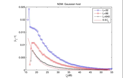
var-ianceΔ2/(3L). Thus,ljtends to 1 - 0.5/ζjas L®∞orΔ ® 0 (i.e.,ζj® ∞). Figure 6 plots the curves of the true
average error |lj- 1| versusζjfor different L, as well as
the limit 0.5/ζj. Notably, the gap between the factor lj
and its limit becomes smaller and smaller as L and DWR increase. Over the most interesting range of ζj
from 25 dB to 50 dB, the value of |lj- 1| is less than
0.01 for all the values of Ltested. From Figure 4a, it is observed that the valumetric scaling with |lj- 1|<0.01
affects the performance of NDM so less that no decod-ing error is made.
As to the constant change withE{qej}, we have a suffi-cient condition thatE{qej}< /2for making no error. Considering the statistical properties of qej, it is possible
to resort to the CLT to show that for largeL, the sam-ple mean q¯ejcan be accurately modeled by a Gaussian PDF with zero mean and variance Δ2/(3L). Thus, the probability that|¯qej|<
2holds can be computed as
P(|¯qej|< /2)≈1−2(−
3L/4). (23)
Since the probability in (23) approaches the value of 1 asL increases, NDM can present a zero probability of error as the original DM for largeL in the absence of channel noise. Figure 7 shows the plots of the BER as a function ofL. As shown in Figure 7, the probability of error sharply decreases to 0 as L increases. And the agreement of theoretical results with simulations is excellent.
Next, we will analyze the performance of NDM in noise channel. The received signalzjhas the formzj=
15 20 25 30 35 40 45 50 55
0 0.005 0.01 0.015 0.02 0.025
j(dB)
|
j
−
1|
NDM: Gaussian host
L=32 L=96 L=640 0.5/j
yj +νj, where νjis an unknown noise source with zero
sample mean andνjand yjare orthonormal. Since NDM
is invariant to valumetric scaling and constant change attacks, it’s sufficient to consider the case. To measure the impact of the noise, we will follow the popular watermark-to-noise ratio (WNR), defined as ξj||yj−xj||2/||νj||2for the jth subvector. Applying the
normalization operation tozjyields
zj− ¯zja Szj
=λjQbj
xj− ¯xja Sxj
+νj+q¯eja (24)
with λj=λj
ζjξj
ζjξj+ 1
, νj=
ζjξj
ζjξj+ 1
νj sxj
, and
¯
qej =−λjq¯ej. Expression (24) illustrates that NDM
under-goes the composite attacks as considered in (3). There-fore, the previously obtained theoretical results can be used to predict the performance of NDM.
Generally speaking, the factor λjin (24) is
approxi-mately equal to the value of 1 by the fact thatζjξj≫ 1
holds in practical applications. Figure 8 shows that the value of|λj−1|is rather less even for serious distortions
(e.g., WNR = -10 dB). On the other hand, for largeL, the effect ofq¯ejin (24) can be neglected. Based on these two considerations, the increase of BER is mainly derived from the termνjin (24). As a result, we can
draw the conclusion that NDM almost resists the same amount of noise as the original DM. Figure 9 illustrates the performance difference between NDM and DM under the additive noise attacks. As can be seen, NDM performs slightly worst than DM when the WNR is within the range [-1 dB, 3 dB], but outperforms it once WNR is lower than -1 dB. In principal, their perfor-mance is very close in this regard. Under the light of the above analysis we conclude that NDM achieves the performance approximately equal to DM, still keeping invariance against valumetric scaling and constant change attacks.
6 The improvement of NDM
The previous analysis shows that when lj ≠ 1 and ¯
qej = 0the two factors have the negative impact on the performance of NDM. Thus, the influence of them should be decreased or eliminated so as to obtain the improved performance. Based on this idea, we present the improved NDM (IM-NDM) in the sequel.
5 10 15 20 25 30
0 0.05 0.1 0.15 0.2 0.25 0.3 0.35 0.4 0.45
L
BER
NDM: Gaussian host,DWR=37dB
Empirical values Analytical prediction
In IM-NDM, the watermarked vector is generated by weighting the quantization error signal and adding it back to the host signal. The modified embedder is expressed as
yj=λjSxj(xj+αj·qej) +ηja, (25)
whereajdenotes the weight vector whose element is
between 0 and 1, andαj·qejindicates that each dimen-sion ofajis multiplied by the corresponding dimension
ofqej· Similarly to (18) and (19), it is derived that
λj= (1 +S2qej+ 2q
T ejx
j/L)−
1
2 (26)
and
ηj=¯xj−λjSxjq¯ej. (27)
Note that NDM is a special case of IM-NDM with aj
=a. The weight vectorajplays an important role in the
performance of IM-NDM. Through a careful choice of aj, the influence of both lj and q¯ej in (25) can be decreased (or even eliminated), and at the same time the distortion-compensation (DC) mechanism is intro-duced. The latter is proved to be an effective way to
improve the performance of quantization-based water-marking [1].
By lettinglj= 1 andηj=x¯j, we have
(αj·qej)
T(α
j·qej+ 2x
j) = 0 (αj·qej)
T
a= 0. (28)
Taking use of one solution of (28) in (25) allows us to eliminate the negative impact ofljandhj. Obviously, it is
easy to obtain one solution of (28) for one of the two equations in (28) is linear. If (28) has multiple solutions, an appreciate one should be chosen by the performance of IM-NDM. Obtaining the appropriate solution foraj
and investigation of its effect on watermarking perfor-mance is beyond the scope of this article and is a good direction for future research. If (28) has none solution,aj
should be chosen to minimize |lj- 1| under the situation
ηj=x¯j. This is a constraint optimization problem and can
be solved using the Lagrangian multiplier method. Figure 9 illustrates the performance of IM-NDM described above under the additive noise attack, together with DC-DM, and the distortion compensated NDM (DC-NDM), namely IM-NDM taking the same weight for each element ofqej, where the DC value is set
−25
−030 −20 −15 −10 −5 0 5 10
0.05 0.1 0.15 0.2 0.25 0.3 0.35 0.4 0.45 0.5
j(dB)
|
j
−
1|
NDM: Gaussian host and noise, L=32
j=25dB
j=30dB
j=35dB
to 0.66 for the latter two schemes. Obviously, DC-NDM almost presents the same robustness as DC-DM against weak attacks, and performs a little better facing very ser-ious distortions (WNR<-4 dB). And they are noticeably outperformed by IM-NDM.
7 Experimental results
In this section, a series of experiments are conducted on real images to evaluate the validity of analytical deriva-tions and performance of the proposed method.
7.1 Theoretical verification
In the experiments, we use three standard images, shown in Figure 10. The DM method is implemented in the
spatial domain so as to observe its performance without the impact of transform operations. Specifically, all pixels of one image are rearranged in a vector as the host signal. A random binary message is embedded into the host vec-tor by DM when given the quantization stepΔ, the dither valuedand the number of dimensionsL. The watermark-ing algorithm is tested under the composite attacks of valumetric scaling with the factorr, constant change with the valuecand additive noiseνfollowing the distribution GGD(bν; 0,sν). The distribution parameters of image
pix-els used for the computation of theoretical BERs are dis-played in Table 1, which are obtained by the maximum likelihood estimator [15]. The experimental results are summarized in Figure 11 forL= 32,Δ= 8, andd= 0.
−8 −6 −4 −2 0 2 4
0 0.05 0.1 0.15 0.2 0.25 0.3 0.35 0.4 0.45 0.5
WNR(dB)
BER
Gaussian host and noise: L=32, and DWR=35dB
DM
DC−DM
NDM
DC−NDM
IM−NDM
Figure 9BER as a function of AWGN for Gaussian host.
Figure 11a depicts the plots of BER as a function of the scaling factor r for each image. On the Crowd image, which has the smallest shape parameter among the tested images, DM achieves the best performance. This behavior is consistent with the results in Figure 5a. The shape parameter of the Lena image is larger than one of Mandrill, but better performance is achieved on the Lena image. This can be explained as follows. The valumetric scaling operation introduces the serious dis-tortions on the Mandrill image with a distinctively large mean luminance. As a result, not only the performance gain caused by the host PDF shape cancels out but also
the BER grows up. The analytical curves closely fit the empirical data for the Lena and Mandrill images. By contrast, the prediction accuracy becomes slightly worse for the Crowd image. That is mainly due to the fact that the GGD is a poor model for this image. Figure 11b illustrates the sensitivity of DM to the addition/subtrac-tion of a constant luminance value while fixing r and sν. In the test, DM performs closely for all the test
images. That is, the performance of DM with respect to constant change attack is insensitive to the statistical properties of host signal. It is remarkable that the empirical performance of DM is predicted by the theo-retical results with a high degree of accuracy. The plots of BER versus the standard deviation sν are shown in
Figure 11c for bν= 1 and Figure 11d for bν = 8 while
fixing r andc. As to the attack, the obvious perfor-mance difference is observed between different images. The effect is actually caused by the valumetric scaling operation, and thus can be removed by setting r = 1. Comparing Figure 11c with Figure 11d, it becomes clear
Table 1 Mean, variance, and shape parameter of image pixels
Image μx sx bx
Crowd 85.2 50.9 1.5
Mandrill 129.1 42.4 3.3
Lena 99.1 47.9 10.6
0.95 0.96 0.97 0.98 0.99 1 1.01 1.02 1.03 1.04 1.05 0.1
0.2 0.3 0.4 0.5 0.6 0.7 0.8 0.9
ρ
BER
Lena et al.: L=32, Δ=8, d=0
Crowd: Empirical Crowd: Analytical Mandrill: Empirical Mandrill: Analytical Lena: Empirical Lena: Analytical
(a)
−6 −4 −2 0 2 4 6 8
0 0.1 0.2 0.3 0.4 0.5 0.6 0.7 0.8 0.9
c
BER
Lena et al.: L=32, Δ=8, d=0
Crowd: Empirical Crowd: Analytical Mandrill: Empirical Mandrill: Analytical Lena: Empirical Lena: Analytical
(b)
1 2 3 4 5 6 7 8 9 10 0
0.05 0.1 0.15 0.2 0.25 0.3 0.35 0.4
σν
BER
Lena et al.: L=32, Δ=8, d=0
Crowd: Empirical Crowd: Analytical Mandrill: Empirical Mandrill: Analytical Lena: Empirical Lena: Analytical
(c)
1 2 3 4
0 0.1 0.2 0.3 0.4 0.5
σν
BER
Lena et al.: L=32, Δ=8, d=0
Crowd: Empirical Crowd: Analytical Mandrill: Empirical Mandrill: Analytical Lena: Empirical Lena: Analytical
(d)
that the additive noise with a flat PDF is a worst-case attack for DM. This agrees with the observation in Fig-ure 5b. In the two cases, the predictions are desirable, but there are small discrepancies at some points.
7.2 Performance evaluation
We tested the performance of the proposed NDM in terms of imperceptibility and robustness and compared it with DM, DC-DM, Oostveen’s method [10] and RDM [9]. Experiments were carried out on a database of 4000 images from the Corel database, each of dimension 256 ×384. The watermark embedding was performed in the spatial domain in order to see the sensitivity of the tested schemes to constant intensity change. Specifically, we divided the target image into nonoverlapping blocks of size 8×8 and extracted a total of 225 blocks with the highest local variance. Each of the extracted blocks was modulated with two random message bits, so a total of 450 bits can be embedded into one image. The DC value was set to 0.66 for DC-DM. The L2 vector norm of 50th-order
was used as the division function in RDM.
In the experiment on watermarking imperceptibility, the watermark energy induced by all the tested schemes is kept the same and in this case the watermarked images’ quality is assessed with several objective image quality metrics. The weighted peak signal-to-noise ratio (wPSNR) and the total perceptual error (TPE) are used to measure the global image quality, as well as the num-ber of blocks greater than the first local perceptual error threshold (NLPE1) and the second local perceptual error threshold (NLPE2) to measure the local image quality. The parameters for them take the default values as suggested in Checkmark [16]. Table 2 reports the experimental results averaged over all the test images when the DWR is fixed at 21 dB.
As shown in Table 2, among all the tested watermark-ing schemes, NDM and its improved version offer the highest wPSNR values (in dB), the smallest TPE, NLPE1, and NLPE2 values for the same watermark energy. They all indicate that the performance of NDM, in terms of imperceptibility, is better than that of other ones. This is because the adaptive quantization step size is chosen to be proportional to the local variance of the host image in NDM (see (17)). The image quality
produced by IM-NDM degrades when compared with NDM. The situation also presents between DM and DC-DM. This is attributed to the fact that a large quan-tization step is used for watermark embedding with dis-tortion compensation. Surprisingly, RDM manifests the worst performance in this regard.
In what follows, the watermark robustness will be evaluated with respect to some typical image processing operations. The watermarked images were produced by the tested schemes when fixing DWR at 21 dB. All the given BERs are averaged over the test set of images, except otherwise indicated.
Figure 12 shows the robustness to amplitude scaling for all schemes. Clearly, except the conventional DM and DC-DM, the others manifest strong robustness against this attack. Particularly, the lowest values of BER are achieved by IM-NDM over the whole range of scaling factorrtested. However, whenrexceeds 1.2, the robust-ness of IM-NDM goes down slightly. That can be attribu-ted to the increasing rounding and clipping distortions.
Figure 13 illustrates the sensitivity of all schemes to the addition/subtraction of a constant luminance value c. It can be seen that both DM and DC-DM are very fragile to constant change attack. The BER of them sharply increases to 1 when cgets close to 10 or -10. Although Oostveen’s method and RDM perform better than the original QIM schemes, they are still sensitive to this kind of attack. Our methods are evidently more robust in this regard than other ones. They are almost invariant to constant change and approximately keep the BER of 0 over the range ofctested.
The robustness to AWGN is shown in Figure 14 for each watermarking scheme. In this regard, NDM clearly outperforms Oosteen’ method and RDM. Comparing with DM, NDM achieves higher BER for weak noise. This can be explained by the fact that the introduced noise causes the errors in the estimation of the quanti-zation step size for NDM. However, as the noise becomes strong, the BER of DM grows rapidly and is finally lower than one of NDM. The situation is in accordance with the analytical results in Section 5.2. Note that IM-NDM behaves like NDM but presents the improved performance.
The robustness of NDM against AWGN was also tested on the Lena image to verify the analytical deriva-tions for NDM. Since the performance of NDM depends on the local variance of the host image, the empirical BER can not be accurately predicted by exploiting the information from a certain image block. Thus, for the computation of the theoretical BER, we chose three image blocks with different variance: the middle one is around the average variance over those image blocks for watermark embedding and other two ones are respec-tively a little larger and smaller than it. The theoretical
Table 2 Watermark imperceptibility assessment in use of several image quality metrics
Metrics DM DC-DM Oostveen’s RDM NDM IM-NDM
0.5 0.6 0.7 0.8 0.9 1 1.1 1.2 1.3 1.4 1.5 0
0.1 0.2 0.3 0.4 0.5 0.6 0.7
Scaling factor
BER
DWR=21dB, L=32
DM
DC−DM
Oostveen RDM NDM
IM−NDM
Figure 12BER as a function of amplitude scaling.
−030 −20 −10 0 10 20 30
0.1 0.2 0.3 0.4 0.5 0.6 0.7 0.8 0.9 1
Constant change
BER
DWR=21dB, L=32
DM DC−DM Oostveen RDM NDM IM−NDM
and empirical results are depicted in Figure 15. As can be seen, the upper analytical curve relatively fits well to empirical observations in the weak noise case, and other two curves respectively do well for the moderate noise and strong noise cases respectively. In principle, the the-oretical results are effective for real image.
The sensitivity to JPEG compression is investigated in Figure 16. In this test, NDM performs a little worse than DM. IM-NDM improves the robustness of NDM, but still falls behind DC-DM. It is worth seeing that RDM has superior performance with respect to JPEG compression. That can be explained by the nature of JPEG compression. Unlike the AWGN, JPEG compression is an image-depen-dent processing operation. The goal of it is to reduce an image file size without noticeable image quality degrada-tion. Thus, the perceptually unrelevant data are removed from an image after compression. The test results of image quality reveals that RDM modifies the image data to be easily noticed more largely than other ones, so that it is impaired less by compression. The situation is opposite for NDM. If the perceptual quality is set to be same for all the tested schemes, it is reasonable to believe that NDM will manifest better performance.
NDM is just a basic watermarking algorithm like DM. The above tests allow us to evaluate its performance base-line and the implementation is coarse. If one wants to design a NDM based watermarking scheme for practical
applications, some effective technologies on performance improvement should be carried out, such as the choice of transform domain, the use of error-correction coding, etc. Several image-adaptive DM algorithms are presented by exploiting the characteristics of the human visual system in [11]. The same ideas can be straightforwardly applied to improve the performance of NDM. Recently, a new Loga-rithmic QIM is developed by introducing theμ-Law con-cept in [4]. NDM can also attempt to use the concon-cept for the improvement of performance.
8 Conclusion
The contribution of this article is twofold. First, we have been theoretically evaluated the performance of DM facing the combination of valumetric scaling, additive noise and constant change. The analyzes were developed under the assumptions that both the host vector and the noise vector have i.i.d components and the two vectors are independent. We accurately derived the general expressions of the PDFs of the watermarked signal, the attacked signal and the extracted signal. By these derived PDFs, the decoding error probability was gener-ally expressed in closed form. The specific analytical results were presented for the case of generalized Gaus-sian host and noise. Moreover, the theoretical results can be easily extended by modeling the host and noise signals with other distributions.
0 2 4 6 8 10 12 14 16 18 20
0 0.05 0.1 0.15 0.2 0.25 0.3 0.35 0.4 0.45
Standard deviation of the AWGN
BER
DWR=21dB, L=32
DM DC−DM Oostveen RDM NDM IM−NDM
According to our analyzes, DM is largely vulnerable to valumetric scaling. And constant change and additive noise give rise to the relatively large performance loss of DM by combining them with valumetric scaling. Parti-cularly, we have seen the effect of statistical properties of the host and noise signals on the performance of DM. The more impulsive the PDF shape of the host sig-nal, the more robust DM is to valumetric scaling. The more flat the PDF shape of the noise source, the more sensitive DM is to additive noise. Simulations on artifi-cial signals and real images show us that the bit-error probability is accurately predicted by the given theories for a wide range of host and noise PDF shapes. These can ultimately guide the design of efficient watermark-ing algorithms based on DM.
Second, a novel watermarking method, called NDM, has been developed. In the method, the normalized host signal vector is constructed for quantization. The NDM achieves its theoretical invariance to both valumetric scaling and constant change, but leads to small perfor-mance loss in the absence of channel noise. The BER of NDM against additive noise can be predicted by apply-ing the presented theoretical results of DM. Further, the
NDM is improved by weighting the quantization errors. Experiments on images demonstrate that the proposed method achieves better watermark imperceptibility and extremely strong robustness against valumetric scaling and constant change attacks comparing with the original QIM schemes and other improved versions.
Appendix
Here, we will derive the integration terms in (10) and (11) when the attacking noise obeys the distribution GGD(bν; 0, sν). For this purpose, using a variable t
instead ofμjk, they are, respectively, rewritten as
−
|u|pν(t−u)du=
0
u(pν(t+u) +pν(u−t))du
=
−t
−t
upν(u)du+
t+
t
upν(u)du
+t
⎛ ⎝
−t
−t
pν(u)du−
t+
t
pν(u)du)
⎞ ⎠
(29)
0 2 4 6 8 10 12 14 16 18 20
0 0.05 0.1 0.15 0.2 0.25 0.3 0.35 0.4 0.45
Standard deviation of the AWGN
BER
Lean: DWR=30dB, L=32
Empirical
M−T
L−T
S−T
and
−
u2p
ν(t−u)du=
t+
t−
(u2−2tu+t2)p
ν(u)du
= t+
t−
u2p
ν(u)du−2t
t+
t−
upν(u)du+t2
t+
t−
pν(u)du
(30)
Thus, achieving the two integrations can be attributed to the computation of I(t1, t2), defined as I(t1, t2)
t2
t1 u
lp
ν(u)duwithlbeing an integer. Considering the case oft1≥0 andt2≥0, we have
I(t1, t2) = κνβν
2(βν−1) t2
t1
ule−|κνu|βν
du
= 1
2(β−1
ν )κνl
(κνt2)βν
(κνt1)βν
ul+1βν −1e−udu
=γ((l+ 1)β −1
ν , (κνt2)βν)−γ((l+ 1)βν−1, (κνt1)βν)
2σ−l ν
((β−1
ν ))2−l((3βν−1))l
(31)
where the first equality follows from (13) and the final equality follows from the definition of the lower incom-plete gamma function.
In the case oft1≤0 andt2 ≤0,I(t1,t2) has the form
I(t1,t2) = κνβν
2(β−1
ν )
t2
t1
ule−(−κνu)βνdu
=(−1)
l+1κ
νβν
2(βν−1)
−t2
−t1
ule−(−κνu)βνdu
=γ((l+ 1)β
−1
ν , (−κνt2)βν)−γ((l+ 1)βν−1, (−κνt1)βν)
2(−1)l+1σ−l ν
((β−1
ν ))2−l((3β−1
ν ))l
(32)
where the final equality follows from (31). Last, whilet1 ≤0 andt2≥0, it follows that
I(t1, t2) = κνβν
2(βν−1) ⎛ ⎝
0
t1
ule−(−κνu)βνdu+
t2
0
ule−(−κνu)βνdu
⎞ ⎠
=γ((l+ 1)β
−1
ν , 0)−γ((l+ 1)βν−1, (−κνt1)βν)
2(−1)l+1σν−l
((βν−1))2−l((3βν−1))l
+γ((l+ 1)β
−1
ν , (κνt2)βU)−γ((l+ 1)βν−1, 0)
2σ−l ν
((β−1
ν ))2−l((3β−ν1))l
(33)
20 30 40 50 60 70 80 90 100
0 0.05 0.1 0.15 0.2 0.25 0.3 0.35 0.4 0.45
JPEG quality
BER
DWR=21dB, L=32
DM
DC−DM
Oostveen RDM NDM
IM−NDM
where the final equality is due to (31) and (32). Com-bining the three cases, a unified form ofI(t1,t2) is
I(t1, t2) = γ((l+ 1)β
−1
ν , 0)−γ((l+ 1)βν−1,|κνt1|βν)
2(sgn(t1))l+1σν−l
((βν−1))2−l((3β−ν1))l
+ γ((l+ 1)β −1
ν ,|κνt2|βν)−γ((l+ 1)βν−1, 0)
2(sgn(t2))l+1σν−l
((βν−1))2−l((3β−ν1))l
(34)
By the formula (34) and the CDF of the GGD, (29) becomes
−
|u|pν(t−u)du=γ(2β−
1
ν ,|κ(t−)|βν)−γ(2βν−1,|κt|βν)
2σν−1
(βν−1)(3βν−1)
+γ(2β−
1
ν ,|κ(t+)|βν)−γ(2βν−1,|κt|βν)
2σν−1
(βν−1)(3βν−1) + (2ν(t)−ν(t−)−ν(t+))t
and (30) becomes
−
u2pν(t−u)du=γ(3β
−1
ν , 0)−γ(3βν−1,|κν(t−)|βν)
2sgn(t−)σ−2
ν (3β−1
ν )
+γ(3β
−1
ν ,|κν(t+)|βν)−γ(3β−1
ν , 0)
2sgn(t+)σ−2
ν (3β−1
ν )
−(γ(2βν−1,|κ(t+)|βν)−γ(2βν−1,|κ(t−)|βν))t
σ−1
ν
(βν−1)(3βν−1) + (ν(t+)−ν(t−))t2
Acknowledgements
This study was supported by the National Natural Science Foundation of China (Grant No. 60803122, 61103018), by the Natural Science Foundation of Jiangsu Province (Grant No. BK2011442), by the Innovative Foundation of Yangzhou University (Grant No. 2011CXJ023), by the Opening Project of State Key Laboratory of Digital Publishing Technology, and by the Opening Project of State Key Laboratory of Software Development Environment (Grant No. SKLSDE-2011KF-08). The authors would like to thank the anon-ymous reviewers for their detailed comments that improved both the editorial and technical quality of this article substantially.
Abbreviations
AWGN: additive white Gaussian noise; CDF: cumulative distribution function; CLT: central limit theorem; DC: distortion-compensation; DC-DM: distortion compensated dither modulation; DC-NDM: distortion compensated NDM; DM: dither modulation; DWR: document-to-watermark ratio; GGD: generalized Gaussian distribution; i.i.d.: independently and identically distributed; IM-NDM: improved NDM; LQIM: logarithmic QIM; NDM: normalized dither modulation; NLPE1: number of blocks greater than the first local perceptual error threshold; NLPE2: number of blocks greater than the second local perceptual error thresh-old; PDF: probability distribution function; PMF: probability mass function; BER: bit error rate; QIM: quantization index modulation; r.v.: random variable; RDM: rational dithered
modulation; SCS: scalar Costa scheme; STDM: spread transform dither modulation; TPE: total perceptual error; WNR: watermark-to-noise ratio; wPSNR: weighted peak signal-to-noise ratio.
Author details
1School of Information Engineering, Yangzhou University, Yangzhou 225009, China2State Key Laboratory of Digital Publishing Technology, Chengfu Road 298, Beijing 100871, China3State Key Laboratory of Software Development Environment, Beihang University, Beijing 100191, China
Competing interests
The authors declare that they have no competing interests.
Received: 20 June 2011 Accepted: 2 March 2012 Published: 2 March 2012
References
1. B Chen, GW Wornell, Quantization index modulation: a class of provably good methods fordigital watermarking and information embedding. IEEE Trans Inf Theory.47(4), 1423–1443 (2001). doi:10.1109/18.923725 2. JJ Eggers, R Bauml, R Tzschoppe, B Girod, Scalar costa scheme for
information embedding. IEEE Trans Signal Process.51(4), 1003–1019 (2003). doi:10.1109/TSP.2003.809366
3. JP Boyer, P Duhamel, J Blanc-Talon, Performance analysis of scalar DC-QIM for zero-bit watermarking. IEEE Trans Inf Foren Secur.2(2), 283–289 (2007) 4. NK Kalantari, SM Ahadi, A logarithmic quantization index modulation for
perceptually better data hiding. IEEE Trans Image Process.19(6), 1504–1517 (2010)
5. F Pérez-Gonzàlez, F Balado, JRH Martin, Performance analysis of existing and new methods for data hiding with known-host information in additive channels. IEEE Trans Signal Process.51(4), 960–980 (2003). doi:10.1109/ TSP.2003.809368
6. F Bartolini, M Barni, A Piva, Performance analysis of ST-DM watermarking in presence of nonadditive attacks. IEEE Trans Signal Process.52(10), 2965–2974 (2004). doi:10.1109/TSP.2004.833868
7. F Pérez-Gonzàlez, C Mosquera, Quantization-based data hiding robust to linear-time-invariant filtering. IEEE Trans Inf Foren Secur.3(2), 137–152 (2008)
8. JH Conway, NJA Sloane,Sphere Packings, Lattices, and Groups, (Springer, New York, 1988)
9. F Pérez-Gonzàlez, C Mosquera, M Barni, A Abrardo, Rational dither modulation: a high-rate data-hiding method invariant to gain attacks. IEEE Trans Signal Process.53(10), 3960–3975 (2005)
10. JC Oostveen, AAC Kalker, M Staring, Adaptive quantization watermarking, in Proc of SPIE: Security, Steganography, and Watermarking of Multimedia Contents VI, San Jose, CA,5306, 296–303 (2004)
11. Q Li, IJ Cox, Using perceptual models to improve fidelity and provide resistance to valumetric scaling for quantization index modulation watermarking. IEEE Trans Inf Forens Secur.2(2), 127–139 (2007)
12. A Papoulis,Probability, Random Variables, and Stochastic Processes, (McGraw-Hill, New York, 1991)
13. N Saralees, A generalized normal distribution. J Appl Stat.32(7), 685–694 (2005). doi:10.1080/02664760500079464
14. L Schuchman, Dither signals and their effect on quantization noise. IEEE Trans Commun Technol.CT-12, 162–165 (1964)
15. MN Do, M Vetterli, Wavelet-based texture retrieval using generalized gaussian density and Kullback-Leibler distance. IEEE Trans Image Process.
11(2), 146–158 (2002). doi:10.1109/83.982822
16. S Voloshynovskiy, S Pereira, V Iquise, T Pun, Attack modelling: towards a second generation watermarking benchmark. Signal Process. (Special Issue)
81(6), 1177–1214 (2001)
doi:10.1186/1687-6180-2012-53