Predicting completion risk in PPP projects using big data analytics

Predicting completion risk in PPP Projects using Big Data

Analytics

Abstract:

Accurate prediction of potential delays in PPP projects could provide valuable information relevant for planning, and mitigating completion risk in future PPP projects. However, existing techniques for evaluating completion risk remain incapable of identifying hidden patterns in risk behaviour within large samples of projects, which are increasingly relevant for accurate prediction. To effectively tackle this problem in PPP projects, this study proposes a Big Data Analytics (BDA) predictive modelling technique for completion risk prediction. With data from 4294 PPP project samples delivered across Europe between 1992 and 2015, a series of predictive models have been devised and evaluated using linear regression, regression trees, random forest, support vector machine and deep neural network for completion risk prediction. Results and findings from this study reveal that random forest is an effective technique for predicting delays in PPP projects, with lower average test predicting error than other legacy regression techniques. Research issues relating to model selection, training and validation are also presented in the study.

1 Background

In recent decades, the construction industry has been caught up in the frenzy of the widespread digital revolution that is shaping global landscape (Bilal et al., 2015). More than ever, the industry is witnessing an era of vast accumulation of valuable data needed for making informed decisions (Bilal et al., 2015). The rising availability of electronic data in diverse formats (multi-dimensional (n-D) CAD data, 3D geometric encoded data, graphical data, video, audio, text, etc.) and sizes (terabytes, petabytes etc.) has intensified the adoption of fast technologies with strong analytical capabilities within construction industry (Caldas et al., 2002). One of these frontier technologies is Big Data. Big Data are enormously large dataset that may be analysed computationally to uncover hidden patterns, unknown correlations, trends or preferences (Sagiroglu and Sinanc, 2013). Typically, Big Data has three essential attributes, also known as the 3Vs, which distinguishes it from traditional data sets (Wu et al., 2014). These are (1) Volume (Terabyte, Petabyte, Exabyte etc.); (2) velocity (continuous data streams and fast processing) and, (3) variety (disparate datasets in graphics, texts, pictures, audio, video, graphs etc.). These 3Vs are clearly apparent in most construction project data in recent times, providing opportunities for unravelling useful information from large data sample.

possible outcomes and solution (Boyd and Crawford, 2012). In this study, we examine predictive modelling of completion risk in PPP projects using big data analytics. Gatzert and Kosub (2016) described completion risk in construction projects as the uncertainty that a project will be completed at a contractually agreed date. Recent literatures have examined completion risk analysis in PPP projects using various statistical tools such as Monte Carlo simulation, stochastic method, linear modelling, Project Evaluation Review Technique (PERT), critical path method etc.( Kokkaew and Chiara, 2010; Ching, 2014; Le-Hoai et al., 2008). Despite their immense contributions, most studies have concentrated on few project samples and limited data sources from simple relational databases (Soibelman et al. 2008; Kokkaew and Chiara, 2010; Javed et al., 2013). As such, these studies have either been adjudged deterministic or fixated on identifying generic factors influencing project delay (Kokkaew and Chiara, 2010). This is a major flaw in current completion risk analysis tools, as they remain incapable of identifying hidden patterns and trends in completion risk behaviour that are relevant for accurate forecasting of completion risk across large portfolio of PPP projects. The adoption of Big Data enabled predictive modelling techniques is therefore imperative for accurate prediction of completion risk within this context. These predictive techniques will enable in-depth investigation of the dynamic interaction of underlying factors influencing project delay. In this regard, high precision analytics techniques such as Deep Neural Network (ANN), Random Forest, Support Vector Machine (SVM), Linear Regression, and Regression Trees will be adopted for predictive purposes. The overarching aim of this study is therefore to develop the best Big Data Analytics based predictive model that can be used to estimate delay in PPP projects. In order to achieve the above aim, the following objectives have been identified for the study:

(1)To identify the factors influencing delay in PPP projects and their dynamic interaction in large project samples.

(3)To compare and contrast the predictive performance of these techniques toward completion risk forecasting in large project samples.

This study seeks to examine the behaviour of completion risk across large PPP project portfolio. Using big data driven predictive analyses, 4294 PPP projects between year 1992 and 2015 were examined across Europe for completion risk prediction. Section 2 of this study focused on literature review and examines the application of Big Data Analytics in construction projects, smart cities and IOT. Existing techniques for completion risk evaluation in PPP projects were also discussed under the same section. While section 3 presents the research methodological framework for the study; Section 4 presents analysis of various predictive models for estimating completion risk in PPP projects. This is then followed by the implication for practice, while the last section concludes the study.

2 Literature Review

2.1 Big Data Analytics for Construction Projects and Smart Cities

Data Analytics in the construction sector, academic literature on the topic is only gradually intensifying.

However, a quick review of construction literature revealed two emergent themes of Big Data application in the construction sector namely: Waste Analytics or Waste Management and Smart Cities vis-à-vis IOTs (Internet of Things). Lu et al. (2015) in an investigation into construction waste performance in Hong Kong developed robust KPIs for benchmarking waste generation rate using data from waste disposal records of 5764 projects. The study found demolition works as the largest contributor to waste in Hong Kong, with new building, renovation and maintenance contributing the least amount of waste to landfill. In another relevant literature Bilal et al. (2016) bemoaned existing intelligence-based waste management softwares as lacking the necessary ability to encourage stakeholders. The study also challenged the inappropriate classification of most wastes as mixed wastes under the existing waste management approaches. The study proposed a new Big Data architecture for designing-out waste from projects (by integrating Spark with BIM), and leveraged data from over 200,000 waste disposal records from 900 UK projects. Similarly, Chen et al. (2016) conducted a comparative analysis of construction waste management performances in public and private projects under similar waste management governance. The study analysed over 2 million waste disposal data from 5700 projects and concluded that construction contractors perform better on waste minimization when working on public projects than on private projects. In addition, Brown et al. (2011) investigated the readiness of the construction sector for the adoption of Big Data Analytics using sentiment analysis. Other relevant studies on Big Data in construction and engineering projects include Hampton et al. (2011), Bilal et al. (2015) and Wu et al. (2016).

2.2 Existing Techniques for Evaluating Completion Risk in PPP Projects

Earlier studies have examined completion risk in PPPs including Kokkaew and Chiara (2010); Fight (1999); André Kik (2013); Ye and Tiong (2003); Hoffman (2008). Fight (1999 pp.9) defines completion risk as “the risk that projects do not yield (sufficient) revenues as a consequence of time and budget overruns”. Similarly, Kokkaew and Chiara (2010) refer to completion risk as the uncertainty of construction completion. For the purpose of this study, completion risk is considered as the uncertainty that a project will be completed at a contractually agreed deadline (Project Delay). Many literatures (i.e. Tam et al., 2004; Hoffman, 2008; Shane et al., 2009; Javed et al., 2013) have attributed completion risk to a number of factors within the construction process such as defective design of project, delayed access to project site, shortage in skilled labour etc. Additionally, studies have suggested a number of techniques for completion risk evaluation in construction projects (Ye and Tiong, 2003; Jannadi and Almishari, 2003; Kokkaew and Chiara, 2010; Ching, 2014; Le-Hoai et al., 2008). For instance, Ye and Tiong (2003) argued for the use of incentive schemes (bonuses) to project participants towards ensuring timely completion. The incentive scheme was assumed a function of time and other factors (such as complexity of project, source of revenue etc.), and calculated thus:

B

(

)

λ₁R

(

)

λ₂R

(

)

λ₁R

(

)

λ₂R

(

)

(0≤t<T_e) (T_e≤ t<T_s)(2)

B

(

)

(

) (

)

λ2R

(

)

project schedule and the sequence in which they must be completed. PERT is calculated as:

Meanduration of activity i→ μ_i=

{

6

}

Variance of activity i →Var_i=

{

6

}

Mean of critical path→ μ=

∑

j∈C

μ_{j ,}

where C is a set of critical activities

Variance of critical path→

∑

j∈C

Var_{j ,}

Other completion risk analysis techniques have also been proposed such as Linear-scheduling model (LSM), Critical Path Method (CPM), Gantt Chart, Vertical Production

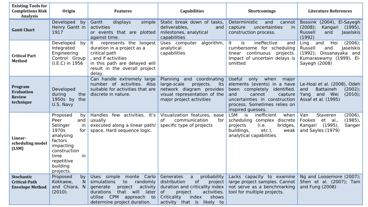
Method (VPM), Line of Balance (LOB) etc. However, despite their wide adoption overtime, André Kik, (2013) argued the reliability of current risk analyses techniques, with their associated inaccuracies regarding completion risk is limited by the use of out-dated analysis techniques (See Table 1 for Exiting techniques for Project Scheduling and Completion Risk Analysis). With the vast accumulation of project data in the construction industry, current risk analysis techniques and softwares including COMFAR III Expert (UNIDO, 1994), CASPAR (Willmer, 1991), EVALUATOR (Abdel-Aziz and Russell, 2006), and INFRISK (Dailami et al., 1999), lack the technological capabilities to hold and analyse large volumes of disparate project data at high speed. As such, a Big Data Analytics (BDA) predictive modelling of completion risk remains the realistic option.

2.3 Big Data Predictive Analytics Techniques

Table 1: Existing Tools for Evaluating Completion Risk in Projects Existing Tools for

Completions Risk

Analysis Origin Features Capabilities Shortcomings Literature References

Gantt Chart

Developed by Henry Gantt in 1917

Gantt displays simple activities

or events that are plotted against time.

Static break down of tasks, deliverables, and milestones, analytical

capabilities

Deterministic and cannot capture uncertainties in construction process.

Bossink (2004), El-Sayegh (2008); Kangari (1995), Russell and Jaselskis (1992)

Critical Part Method

Developed by Integrated Engineering Control Group (I.E.C) in 1956

It represents the longest duration in a project as a critical path

, and if activities

in this path are delayed will result in the overall project delay.

Uses computer algorithm, analytical

capabilities

It is ineffective and cumbersome for scheduling linear continuous projects. Impact of uncertain delays is omitted

Ling and Hoi (2006); Russell and Jaselskis (1992); Dissanayaka and Kumaraswamy (1999), El-Sayegh (2008) Program Evaluation Review technique Developed during the 1950s by the U.S. Navy

Can handle extremely large number of activities. Also suitable for activities that are discrete in nature.

Planning and coordinating large-scale projects. Its network diagram provides visual representation of the major project activities

Useful only when major elements (events) in a have been completely identified. and cannot capture uncertainties in construction process. Sometimes relies on inspired guesses.

Le-Hoai et al. (2008), Odeh and Battaineh (2002); Yang and Wei (2010); Assaf et al. (1995)

Linear-scheduling model (LSM)

Proposed by Peer and Selinger in 1970s for analysing factors impacting construction time in repetitive building projects.

Handles few activities. It’s usually

executed along a linear path/ space, Hard sequence logic.

Visualization features, ease of communication for specific type of projects

LSM is inefficient when scheduling complex discrete projects (i.e. bridges, buildings, etc.), weak analytical capabilities.

Van Staveren (2006), Fookes et al., (1985), Kangari (1995), Sanger and Sayles (1979)

Stochastic Critical-Path Envelope Method

Proposed by Kokkaew, N and Chiara, N (2010).

Uses simple monte Carlo simulations to randomly generate project activity durations that will later utilise CPM approach to determine project duration.

Generates a probability distribution of project duration and criticality index of project activities. Criticality index shows activity that is likely to

Lacks capacity to examine large project samples. Cannot not serve as a benchmarking tool for multiple projects.

cause delay

Benchmarking

Many

company’s In-house method of analysing completion risk

Uses completion time for similar projects to define and arrive at maximum delay time for project

Simply relies on large

samples of historical data It relies on historical dataand benchmark figures that have no predictive value when considering new, large and complex projects

2.3.1 Regression as the Learning Problem

When learning problem is about predicting the quantitative response, the problem is referred to as regression problem. Regression analysis involves single or multiple predictors while predictive modelling. The abstract form of regression analysis is given in Eq. 1 as

Y=ƒ(X)+ϵ 1

Where Y is quantitative response; ƒ is some fixed unknown function of predictorsX, and ϵ is some random error term that is independent of X and has a mean of zero. In Eq. 1, ƒ(X) provides systematic information aboutY and its relationship with ρ predictors. Formally, ƒ(X) can be expressed as shown in Eq. 2

ƒ(X)=β₀+β₁× x₁+β₂× x₂+…+β_p× x_p 2

where x₁, x₂, … , x_p represents ρ predictors andβ₁, β₂,… , β_p represents coefficients of ρ predictors and β0is intercept term. These coefficients quantify association between predictors and the response. In this study, coefficients are derived from a large array of PPP projects using various Big Data Analytics techniques. And to assess predictive performance of model, Residual sum of square (RSS) is usually employed. RSS is the square of difference of distance between predicted value (ŷ) and actual value (y). Eq. 3 describes the RSS for regression analysis.

RSS=

∑

n

(

)

2 3

Big Data Analytics functions for regression of form ƒ(X)=Ε(Y∣x) tends to minimise RSS among all functions from X to Y.

This study starts predictive analysis with multivariate regression analysis as the baseline model for inferential statistics. The R function lm() is used for model development, with basic syntax as lm(y ~ x, data), where y is response, x are predictors, and data is dataset containing x and y. The

superior predictive performance. The predict() function is used to check for test error. Predicted values are plotted to visually inspect variations in predictions. Listing 1 shows R code used to perform regression analysis in this study.

#Creating regression model & checking the sum of squared error for predictions

linearModel <- lm(DELAY ~ .-PROJECT, data = trainPPP) summary(linearModel)

plot(linearModel)

linearPredictions <- predict(linearModel, newdata = testPPP) linearPredictionsDF <- data.frame(pid = testPPP$PROJECT, pred_delay= linearPredictions, ml_func="lm")

linearRSS <- sum((linearPredictions - testPPP$DELAY)^2) rssTB <- data.frame(ml_func = "lm()", rss = linearRSS)

Listing 1: R code for creating and evaluating regression analysis using lm() function

2.3.2 Regression Trees

Tree based models can be used for regression as well as classification problems. Regression trees divides the predictor space (X₁, X₂, X₃, … , X_p) into a set of non-overlapping J distinct regions (R₁, R₂, R₃, … , R_j). A regression tree follows splitting rules, starting at the root and divide down the tree into smaller subsets at each split. A regression tree comprises non-leaf and leaf nodes. Non-leaf nodes are the decision paths to be followed whereas leaf nodes contain decision values. Regions in regression tree are constructed as shapes like boxes or rectangles. Regression tree algorithm tries to find the boxes (regions) that minimize the residual sum of square, given by Eq. 4,

RSS=

∑

J

∑

kϵ Rj

(

)

2

, 4

where ŷ_{Rj is the average value of response in j}th _{box. Since construction of}

algorithms such as recursive binary splitting are used to construct trees in a reasonable computation and time. During recursive binary splitting, every predictor X_{j is selected and a cut s is defined that divides predictor} space into regions, yielding greatest reduction in residual sum of square. Finally, predictor X_jand cut point is chosen for split among predictors ( X₁, X₂, X₃, … ,∧X_{p) that has the lowest residual sum of square. The same}

process repeats for successive splits. This process of tree construction continues until stopping condition is arrived or no regions contain more than five data points. Once regions (R₁, R₂, R₃, … ,¿R_j) are defined, predictions are made for incoming data by simply using the median or mode of data in the region to which new data belong. Regression trees are simplistic, easier to interpret, and have nice graphical representation.

Complexity of regression trees bear significant impact on their predictive power. The deeper the tree, the more likely for it to over-fit test data; hence poor predictive performance. To this end, approaches like pruning regression trees comes in play, where larger tree is grown and is pruned back to obtain an optimal sub-tree. This reduction is achieved through cost complexity pruning (cp), also called as weakest link pruning. The cp considers sub-trees, index by nonnegative parameterα. Whenα=0, tree is

deepest and complex. But as α starts increasing, trees with more nodes pay more prices; hence complexity gets decreasing. So as α increases from 0, branches get pruned. Cost validation is often employed to obtain an optimal value ofα in regression analysis.

In this study, recursive partitioning and regression tree (rpart) library in R is used to fit regression tree model. The size of the tree is decided by cp, which is enforced via cross validation. Regression tree is generated accordingly using train() function for different cp values. The tree model is used to check for test error using predict() function. Predicted values are plotted to visually inspect variations in predictions. Listing 2 shows R code used to achieve these steps in RStudio.

tr.control <- trainControl(method="cv", number=10) cp.grid <- expand.grid(.cp = (0:10)*0.001)

trainTreeModel <- train(DELAY ~ .-PROJECT, data = trainPPP, method="rpart",

trControl=tr.control, tuneGrid = cp.grid)

trainTreePredictions <- predict(trainTreeModel, newdata = testPPP)

trainTreePredictionsDF <- data.frame(pid = testPPP$PROJECT, pred_delay= trainTreePredictions, ml_func="train")

trainTreeRSS <- sum((trainTreePredictions - testPPP$DELAY)^2)

rssTB <- rbind(rssTB, data.frame(ml_func = "train()", rss = trainTreeRSS))

Listing 2: R code for creating and evaluating regression analysis using rpart() function

2.3.3 Random Forest

Regression trees are generally not robust. A small change in data can result in a large change in the model. Non-parametric approaches such as bagging, boosting, and random forest (RF) are mostly used to overcome these limitations. We limit our discussions to RF only. RF improves performance of regression trees by compromising interpretability, i.e., by growing many trees_ƒ^1

(x),_ƒ^2 (x),_ƒ^3

(x), … ,_ƒ^B

(x), and then using average of predictions to obtain low-variance regression model, given by

^

ƒ_avg(x)=1

B

∑

B ^

ƒb

(x) 5

where B denotes the number of trees. RF grows tree by considering a subset m out of ρ predictors. The rule of thumb is to choosem ≈

√

grow trees on training data set. The RF model is used to check for test error using predict() function. Predicted values are plotted to visually inspect variations in predictions. Listing 3 shows R code used to model development and evaluation.

#Building the random forest of trees for predicting risk forestModel <- randomForest(DELAY ~ .-PROJECT, data = trainPPP, mtry=4, importance=TRUE, ntree = 500)

summary(forestModel) plot(forestModel)

importance(forestModel) varImpPlot(forestModel)

forestPredictions <- predict(forestModel, newdata = testPPP) forestPredictionsDF <- data.frame(pid = testPPP$PROJECT, pred_delay = forestPredictions, ml_func="randomForest") forestRSS <- sum((forestPredictions - testPPP$DELAY)^2) rssTB <- rbind(rssTB, data.frame(ml_func = "randomForest()", rss = forestRSS))

Listing 3: R code for creating and evaluating regression analysis using randomForest() function

2.3.4. Support Vector Machine (SVM)

SVM is an ML algorithm with robust regularisation capabilities to generalise to the unseen data with a high degree of accuracy. SVM models can be used for both classification and regression analysis to solve complex and real-world problems. SVM outperforms on data with many attributes even if there are a small number of training examples.

kernels convert training data into points in n-dimensional space and construct numerous linear equations using nonlinear boundaries within the kernel space.

SVM uses epsilon-intensive loss function for regression analysis. The algorithm works by finding a function where more data points lie inside the epsilon-wide insensitivity tube. The epsilon can be customized through SVM settings. SVM balances the margin of error with model robustness to achieve best generalisation for the unseen data.

We used ore.odmSVM() to develop SVM model for regression analysis in this study. Automatic data preparation capabilities of ORE are used for one-hot encoding of categorical variables. The model is trained on training data and evaluated using test data utilizing the ore.predict() function. The predicted values are plotted in figures to inspect variations in predictions. Listing 4 shows R code for performing these steps.

svmFormula <- as.formula("DELAY ~ SECTOR + CONTRACT + NOD + FIMP +

POCI + PODV + PSSL + IMSS + NUSC + PMDS +

PDMD + NSAI + NDSC + PLAD + NDBW + NODP")

svmModel <- ore.odmSVM(svmFormula,data=trainPPP,

"regression", kernel.function="gaussian")

svmPredictions <- predict(svmModel, testPPP[,c(1:16)], supplemental.cols="x")

svmPredictionsDF <- data.frame(pid = testPPP$PROJECT, pred_delay =

svmPredictions$PREDICTION, ml_func="SVM")

rssTB <- rbind(rssTB, data.frame(ml_func = "odmSVM()", rss = svmPredictionsRSS))

Listing 4: R code for creating and evaluating regression analysis using odmSVM() function

2.3.5 Deep Neural Network

Working like a brain, deep neural networks (DNN) is leading among nonlinear regression techniques (Li et al., 2016; Huang et al., 2016). In DNN, response is modelled as a set of intermediate hidden layers that are the linear combination of predictors. DNN employs two obviously different transformations. Firstly, nonlinear function g(.) such as sigmoidal is used

for eliciting the nonlinearity of predictors, which is explained by Eq. 6

hk=g

(

∑

p

xiβjk

)

6

where βcoefficients are similar to that of ordinary linear regression and β_jk is the effect of jth _{predictor on k hidden layer. Secondly, linear}

transformation is applied to convert outcome back to actual values, using the following Eq. 7.

ƒ(X)=γ₀+

(

∑

H

γ_kh_k

)

DNN requires parameter optimization to reduce sum of squared error. To this end, specialized numerical optimization algorithms such as back-propagation (Li et al., 2016) are used. DNN over fits mostly the relationship between predictors and response due to large coefficients, which is combatted through prematurely stopping algorithm or by using penalization techniques like weight decay. DNN tries to minimize RSS for the given value of λ using Eq. 8:

∑

i=1

n

(

)

∑

H

∑

j=0

P

β2_jk

+λ

∑

H

This makes model smoother and less susceptible to over fitting. Another challenge of employing DNN in regression analysis is adverse correlation effect, which is either circumvented manually or by using techniques for feature extraction like principal component analysis (PCA).

We employed neuralnetwork() library in R to develop DNN model. Using

caret() function, hyper-parameter tuning for decay size of DNN is calculated and accordingly model is developed. The DNN model is used to check for test error using compute() function. Predicted values are plotted to visually inspect variations in predictions. Listing 5 shows R code used for model development and evaluation.

#Creating the DNN model

annFormula <- as.formula("DELAY ~ SECTOR + CONTRACT + NOD +

FIMP + POCI + PODV + PSSL +

IMSS + NUSC + PMDS + PDMD +

NSAI + NDSC + PLAD + NDBW + NODP")

annModel <- neuralnet(annFormula, data=trainPPP, hidden=c(10,5),linear.output=T)

annPredictions <- compute(annModel, testPPP[,c(1:16)]) annPredictionsDF <- data.frame(pid = testPPP$PROJECT, pred_delay = annPredictions$net.result, ml_func="ANN") annPredictionsRSS <- sum((annPredictions$net.result - testPPP$DELAY)^2)

rssTB <- rbind(rssTB, data.frame(ml_func = "neuralnet()", rss = annPredictionsRSS))

3 Defining Key Predictors for Completion Risk Analysis using Predictive Modelling

In order to demonstrate Big Data analytics for completion risk forecasting, data of PPP projects between 1992 and 2015 were obtained from database of the European PPP Expertise Centre (EPEC), Monthly Statistics of Construction Building Materials and Components from UK’s Department of Business Innovation and Skills, UK’s Construction Industry Data, Health and Safety in Construction Sector Report of UK, UK’s Office of the National Statistics, European Construction Market data (Euro Area Construction data) etc. Sixteen (16) key predictors causing time overrun in projects were used for the predictive modelling of completion risk. These factors were specifically chosen due to ability to quantify them and their potential impact on delay in construction project delivery (Kokkaew and Chiara, 2010; El-Sayegh, 2008). The factors are articulated in Table 2 below.

Table 2: Key Predictors Influencing Completion Risk (Delay) in PPP Projects

Values Key Predictors Influencing

Completion Risk in PPP Projects

Sources

SECTOR Projects chosen cut across nine (9) sectors of the economy

HM Treasury (2014), NAO (2009)

CONTRAC T

Projects were either procured via turnkey or Design Bid Build

PartnershipsUK.org.uk

NOD Av. No of defects in a construction

project

Buchholz (2004); Teizer et al. (2010);

FIMP % fluctuation in construction material

price index

Javed et al. (2013); Tam et al. (2004)

POCI % change in inflation Ahmed et al. (1999); El-Sayegh

(2008).

PODV % of design variations Kangari (1995); Bossink (2004);

Tatum (1989)

PSSL % shortage in skilled labor Tatum (1989); Bossink (2004);

Tatum (1987)

IMSS % of inferior materials supplied to site

(should be small in value).

Odeh and Battaineh (2002); Errasti et al., (2007)

NUSC No of unforeseen site conditions Dikmen et al., (2007); Flyvbjerg et al.,

(2004)

PMDS % of materials damaged on site Ching (2014); Allen and Iano (2011)

PDMD % Delay in Material delivery Robinson and Scott (2009); Javed et

al. (2013)

NSAI No of site Accidents and injuries Rousseau and Libuser (1997); Shen

et al. (2007)

NDSC No of days for site closure Kaming et al., (1997); Moselhi et al.,

(1997)

PLAD % of liquidated and ascertained

damages in projects

Mohamed (2002); Tam et al. (2004);Tatum (1987)

NDBW No of days with bad weather that

prevented site work

Tatum (1987); Harty (2005); Tatum (1989)

NODP Av. No of disputes among parties El-Sayegh (2008); Russell and

Jaselskis (1992)

1. Sector: The PPP projects selected for the study cuts across nine (9) sectors namely: housing, social care, transport, defence, education, health, waste management, public buildings and others (comprising comprises prisons, leisure facilities, offices, housing, emergency services, courts etc.).

2. Contract Type: The two principal contract types adopted in all the projects analysed are fixed price turnkey and Design Bid Build. Fixed price turnkey ensures a contractor delivers project under a lump sum contract, while accepting completion risk (Hoffman, 2008). On the other hand, Design Bid Build, which is also known as the traditional procurement approach allows a client to contract separate parties for design and construction phases of the project (Bing et al., 2005).

3. Average Number of defects in a construction project: Defects in project delivery is a perennial challenge in the global construction industry. According to El-Sayegh (2008), defects in construction project contribute significantly to construction delay. This could happen as a result of defects in project design or defects due to poor communication between the design managers and the contractors (Zwikael and Ahn, 2011).

4. Percentage (%) fluctuation in construction material price Index: This is often a major concern for contractors as material price fluctuation upsets prior financial forecasts and impacts project timeline, especially where contractor has no parent company cover to bail it out in the event of financial difficulties (Javed et al., 2013). 5. Percentage (%) change in inflation: Similar to fluctuation in

construction material price index, sudden upsurge in general inflation portends great danger to construction budget, which may result in inability to achieve critical milestones on a project (Assaf et al., 1995; Palomo et al., 2007).

2004; Teizer et al. (2010) have argued that frequent changes in design, especially critical components of a project have direct impact on timely completion.

7. Percentage (%) shortage in skilled labour: The direct consequence of not having the right number of skilled manpower to deliver a project is excessive delays in achieving project completion (Aibinu and Jagboro, 2002).

8. Percentage (%) of inferior materials supplied to site: Supply chain is crucial to successful project completion and so is the quality of construction materials supplied to site (Fung et al., 2010). Delays due to discovery of low quality materials supplied to site are not unusual and this may cause serious lag in project schedule (Kaming et al., 1997).

9. No of unforeseen site conditions: These can cause project delay as contractors have to confront site conditions (i.e. topography or underground conditions) not contemplated during the initial construction survey.

10. Percentage (%) of materials damaged on site: Kangari (1995) and Bossink (2004) listed material damage on project site as one of the causes of construction time overrun. Such situations impact both project schedule and construction budget and may pose danger to the project (Bossink, 2004).

11. Percentage (%) Delay in Material delivery: The danger of not having a reliable supply chain is unwarranted disruption in project schedule (Robinson and Scott, 2009). The impact of supply chain delay on a project may be viewed in terms of the percentage of construction duration that is lost to delay in material delivery. 12. Number of site Accidents and injuries: This can be

expressed in terms of man hour loss or site closure due to accidents and its impact on project schedule (Le-Hoai et al., 2008).

construction workers, force majeure, and closure due to potential danger to the public etc. (Flyvbjerg et al., 2004).

14. Percentage (%) of liquidated and ascertained damages in projects: Liquidated damages are financial penalties levied on contractor for breach of contractual obligations (Harty, 2005). This has negative implications for timely delivery of a project, especially where such levy is huge enough to result in financial difficulties that prevents contractor from meeting their obligations to sub-contractors (Bossink, 2004).

15. Number of days with bad weather that prevented site work: Many attimes, protracted and unpredictable weather conditions (high velocity wind, flood etc.) may prevent a project from being completed on time (Fung et al., 2010).

16. Number of disputes among parties: This may be in form of litigation or demand for contractual settlements and is a major factor which often results in project delay (Kangari, 1995). According to Teizer et al. (2010), the frequency of disputed issues on a project has negative implications for timely completion.

In this study, our goal is to develop an accurate model that can be used to estimate completion risk (project delay). In order to achieve this, we assumed a linear relationship between Completion Risk (CR) and the predictors (p). The predictors (p) are thus considered as input variables

(X1,X2,X3… … … … …..Xρ), thereby establishing a directly proportional

relationship between CR as X=(X1,X2,X3⋯Xρ). In other to achieve this, a

linear model is thus developed and formally written as:

CR=f(X)+ϵ 9

f(DELAY)=β₀+β₁× NOD+β₂× FIMP+β₃× POCI+β₄× PODV+β₅× PSSL+β₆× IMSS+β₇× NUSC+β₈× PMDS+β₉× PDMD+β₁₀× NSAI+β₁₁× NDSC+β₁₂× PLAD+β₁₃× NDBW+β₁₄×

NODP

10

Where β_i is the coefficients that will be estimated, where i=0,1,2, … , p

employing Big Data analytics from the large array of data from PPP Project samples.

4 Research Methodology

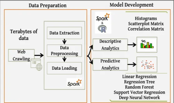
This section explains the methodology employed in the study. After understanding the domain of completion risk in PPP projects, relevant data sources were identified to explore the most critical factors that lead to delay in PPP projects. The methodology-steps have been described in detail under subsequent sections and shown in Fig. 1 below:

Figure 1: Big Data Analytics Workflow for Predictive Risk Modelling

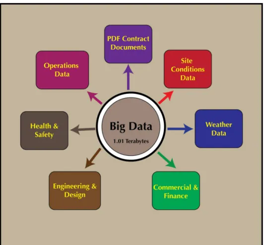
The predictive accuracy of the Big Data models depends on the quality and volume of PPP projects. Data of 4,731 PPP projects were integrated from a large number of structured and unstructured data sources. The data was distributed in a large number of data sources. These include Oracle financials, BIM models, Primavera, Candy, Health & safety, Business objects, Customer relationship management (CRM), and a large body of unstructured documents. These sources were explored to identify relevant data, structures and formats to enable the database design. Fig 2 shows types and sources of data of PPP projects used in the study. This effort has resulted in the exploration of 1.01 terabytes of data for analysis. This data fulfills all 3V’s of the Big Data that is volume, variety and velocity.

4.2 Data pre-processing and integration

Data integration task is found the toughest in the overall risk analytics experience. A variety of syntactical and semantic heterogeneities were resolved (Halevy et al. 2005; Doan & Noy 2004). To ensure data completeness, machine learning (ML) programs were used to predict missing values for predictors like average defects (Bishop 2006; Goldberg & Holland 1988). Data were standardized with vocabularies for construction sectors and contract types. Automatic conversion is augmented to deal with inappropriate interpretations especially for date columns. The data normalization is carried out by formula given in Eq. 11.

X '_i= Xi−Xmin

Xmax−Xmin

11

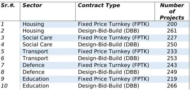
where X '_i is the scaled result of X_i, X_min is the smallest value of X, and X_max is the largest value of X . The final data analytic sample is restricted to 4,294 PPP projects, which is eventually loaded onto Apache Spark—a resilient cluster computer engine for Big Data Analytics. Table 3 shows distribution of projects across sectors and contract types. SparkR is used for data analysis and R ggolot2 package is used for visualisation.

Table 3: Data Analytic Sample of PPP Projects used for Big Data Analytics

Sr.#. Sector Contract Type Number

of Projects

1 Housing Fixed Price Turnkey (FPTK) 200

2 Housing Design-Bid-Build (DBB) 261

3 Social Care Fixed Price Turnkey (FPTK) 227 4 Social Care Design-Bid-Build (DBB) 250 5 Transport Fixed Price Turnkey (FPTK) 233

6 Transport Design-Bid-Build (DBB) 253

7 Defence Fixed Price Turnkey (FPTK) 243

8 Defence Design-Bid-Build (DBB) 249

9 Education Fixed Price Turnkey (FPTK) 219

11 Health Fixed Price Turnkey (FPTK) 190

12 Health Design-Bid-Build (DBB) 251

13 Waste

Management Fixed Price Turnkey (FPTK) 238 14 Waste

Management Design-Bid-Build (DBB) 261 15 Public Buildings Fixed Price Turnkey (FPTK) 225 16 Public Buildings Design-Bid-Build (DBB) 260 17 Others Fixed Price Turnkey (FPTK) 232

18 Others Design-Bid-Build (DBB) 236

Total Data Analytic Sample: 4294

4.3 Descriptive Analytics

We started with exploratory analysis to develop better understanding of the overall PPP projects data. Descriptive analytics is applied to describe main features of the dataset. Important facts are elaborated to get initial impressions of data. Numerical summaries and graphical methods are used. Histograms, boxplots, and scatterplots are drawn to see the fitness of data for predictive modelling.

4.4 Predictive Analytics

Descriptive analytics sets the stage for more flexible predictive analysis, where a series of predictive models were developed using various Big Data Analytics techniques and evaluated for their predictive performance. The data are split across training and test sets using sample() function. We initially developed multivariate linear regression model to understand the interactions of predictors on response. This model is treated as the baseline model. To improve upon the predictive performance of linear model, regression trees were employed. We found different behaviour of delays across different sectors and contract types, which are not fully described by linear regression model.

predictive modelling, we employed random forest to see if they improve the predictive performance by growing 500 trees. Support vector machine (SVM) was also employed to ensure good classification of the data sample. Finally, we brought the deep learning based predictive modelling technique called deep neural networks (DNN). DNN is a black box approach that knows how to process predictors to obtain more accurate matching response. For each model, hyper-parameter tuning is performed and approaches like cross validation was employed to devise a robust model development strategy. These models were plotted using R gglot2

library for evaluating their performance in terms of decreasing the test error. It is shown that random forest is very robust and viable option to employ for estimating the completion risk in the PPP projects.

4.5 Attribute importance and ranking

Since these models employ different model development strategies, they ranked the attributes differently. To aggregate these ranking, a reliable total ranking scheme is devised. The scheme used p-value, Gini, impurity, ranked agreement factor (RAF), and percentage ranked agreement factors (PRAF) for ranking predictors for the completion risk prediction.

5 Analysis and Findings

5.1 Big Data Descriptive Analytics

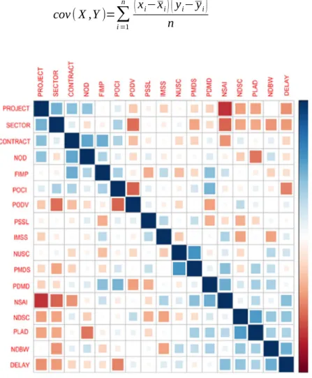
and West, 1994). According to Casella et al. (2013), positive covariance indicates positive linear relationship whereas negative values mean negative linear relationship. Covariance is calculated by the Eq. 12 and colour coded in the Fig. 3.

cov(X ,Y)=

∑

n

(

i−xi

) (

)

n

12

Figure 3: Correlation plot depicts covariance between variables in PPP projects

predictive modelling. However, some variables have strong covariance, like number of days with bad weather NDBW and unforeseen site condition (UNSC). This shows collinearity issue between these variables and informs that these variables tend to add similar predictive capabilities twice. As a result, we dropped NDBW for UNSC to reduce the complexity of the model in order to achieve higher predictive performance.

5.2 Big Data Analytics for Estimating Completion Risk in PPP Projects

In the remainder of this paper, we discuss the development of predictive models for completion risk estimation. Since a single model might not be able to entirely capture the true relationship of different KPIs selected in this study with respect to delays in PPP projects, a mix of linear as well as non-linear Big Data analytics techniques are employed during model development. These techniques have really moved our understanding of completion risk to the next level. In addition, a robust completion risk estimation model is developed for assessing delays in the future PPP projects. Subsequent sections provide more details of these models and their comparisons.

5.3 Multivariate Linear Regression

An important reason behind starting with linear regression is to understand the way delay in PPP projects are influenced by myriad factors. In this case, we estimated ƒ not for the purpose of predicting completion risk in PPP projects. Instead the objective is to understand the relationship between predictor ρ and responseY or more specifically to know how Y changes as a function of ρ. So _{ƒ is not treated as a black box}^

rather, an elaborate description of its exact form. Listing 5 shows the summary of linear regression model.

Call:

lm(formula = DELAY ~ ., data = trainPPP)

Residuals:

-0.73954 -0.07309 0.00192 0.05645 0.71047

Coefficients:

Estimate Std. Error t value Pr(>|t|)

(Intercept) 0.3757610 0.0172054 21.840 < 2e-16 *** SECTOR1 0.0072317 0.0105143 0.688 0.49164 SECTOR2 -0.0096546 0.0104830 -0.921 0.35714 SECTOR3 0.0005468 0.0102727 0.053 0.95755 SECTOR4 0.0100831 0.0104072 0.969 0.33270 SECTOR5 -0.0043815 0.0107594 -0.407 0.68388 SECTOR6 -0.0073937 0.0103638 -0.713 0.47565 SECTOR7 0.0018448 0.0103175 0.179 0.85810 SECTOR8 0.0103248 0.0105442 0.979 0.32757 CONTRACT1 0.0142038 0.0049633 2.862 0.00424 ** NOD 2.4175803 1.1975378 2.019 0.04361 * FIMP -0.1712855 0.0804999 -2.128 0.03344 * POCI 0.0040691 0.0076285 0.533 0.59380 PODV 0.7175872 1.1699697 0.613 0.53970 PSSL -1.1511576 0.6664203 -1.727 0.08421 . IMSS -0.4591695 0.9651310 -0.476 0.63428 NUSC 5.9326532 1.2714082 4.666 3.21e-06 *** PMDS -1.9396845 0.8848595 -2.192 0.02846 * PDMD -4.8422194 0.5106527 -9.482 < 2e-16 *** NSAI -4.1452338 1.2620944 -3.284 0.00103 ** NDSC -1.0147283 1.0164924 -0.998 0.31824 PLAD 11.3065432 1.3579018 8.326 < 2e-16 *** NDBW -6.7006330 0.5704384 -11.746 < 2e-16 *** NODP 0.0012832 0.0074467 0.172 0.86320

---Signif. codes: 0 ‘***’ 0.001 ‘**’ 0.01 ‘*’ 0.05 ‘.’ 0.1 ‘ ’ 1

Residual standard error: 0.1283 on 2756 degrees of freedom Multiple R-squared: 0.6927, Adjusted R-squared: 0.6902 F-statistic: 270.1 on 23 and 2756 DF, p-value: < 2.2e-16

Listing 4: Summary of the Fitted Multivariate Regression Model for Risk Estimation

As mentioned earlier, sector and contract type are categorical variables, dummy variables are created automatically for each of their elements. The intercept term (β₀=4.028_{) is implicitly added to the model. Generally,}

set. The same applies to the contract types as well. Interestingly, the model does not describe the relationship of sectors to delays, which is reported by higher p-values (0.49164, 0.35714, 0.95755, 0.33270, 0.68388, 0.47565, 0.85810, and 0.32757) of all sectors respectively. In contrast, contract type has virtually zero p-value (0.00424), which indicates strong correlation in predicting delays. The implication of this is that delay in project varies based on contract type.

The parameter estimation is computed using ordinary least squares. The

Estimate column shows parameter estimation for predictors and Std. Error displays standard error associated with each of these coefficients. This is used for hypothesis testing, using t-distribution column t value, to determine if each coefficient is not statistically different from zero. And if so, then the predictor is removed from the model. Analysis show that associated hypothesis test p-value in Pr (<|t|) values are small for intercept term, contract type, number of defects (NOD), % of fluctuation in materials price (FIMP), number of unforeseen site conditions (NUSC), % materials damage (PMDS), % delay in materials delivery (PDMD), number of site injuries (NSAI), number of days bad weather (NDBW), and number of disputes among parties (NODP). Whereas, the rest of the attributes are removed from the model since they have no significance in predicting delay in PPP projects. A small p-value corresponds to small probability that such a large t value would be observed under the assumption of null hypothesis. In this case, for a given I = 0, 1, 2, …, p-1, the null and alternate hypothesis follow:

H₀:β_i=0versus H_A:β_i≠0

which in this context says that the model is capable to explain 69% variation in the data. And the overall p-value i.e., < 2.2e-16 is small, which indicates that null hypothesis should be rejected.

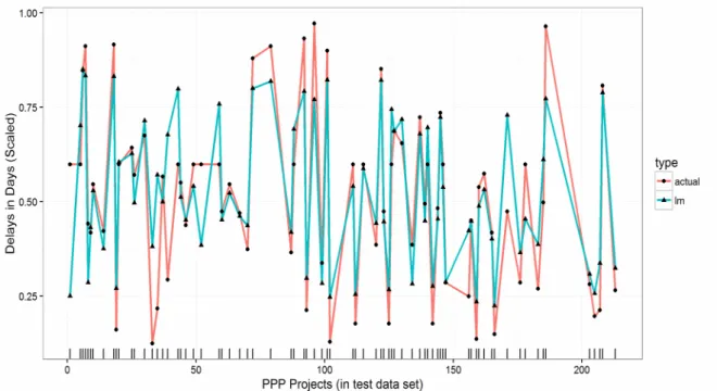
Fig. 4 shows the line plot for observed and predicted delays estimated by the linear regression where R2 is relatively good (69%). However, it is evident that the predictions are not uniformly accurate. To improve upon these, we employed regression trees to capture the non-linear behaviour of predictors on response.

Figure 4: Evaluating observed and predicted delays in the PPP projects

5.4 Regression Trees

parameters are optimised and the regression trees are grown for different

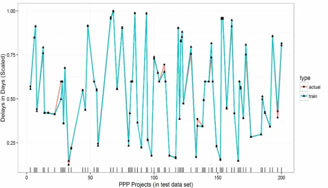
cp values. Here the true power of regression trees comes into play and its effectiveness to uncover non-trivial relationship of predictors could be noticed. Contrary to linear regression, regression tree utilised majority of predictors to develop very strong risk estimation model in the dataset. Similar to regression analysis, contract type is regarded as the most superior predictor in the model; hence taken as the root of the tree. However, the second significant predictor in regression tree is considered the sector, which is totally ignored by the multivariate regression analysis. Regression tree make decisions at various levels based on the sector. So, in this case, the most complex tree is selected by the cross-validation. Fig. 5 shows the line plot for observed and predicted delays for linear regression (with accuracy improved by 79%). It is evident that predictions improved significantly. To improve upon the regression trees, we are employing regression trees to capture the non-linear behaviour of predictors on response (see Fig.6 for regression Tree Model).

5.5 Random Forest

Although, the regression tree model developed for completion risk estimation has improved the test accuracy drastically, it is a non-robust technique and a slight change in data can yield very different regression trees. Hence, we needed to improve the stability of the model by employing random forest. Listing 6 shows the attribute importance summary generated by fitting a random forest of 500 trees on PPP projects data, where two measures of importance are populated. The former is based upon the mean decrease of accuracy in predictions on the out of bag samples when a given variable is excluded from the model. The latter is a measure of the total decrease in node impurity that results from splits over that variable, averaged over all trees. In the case of regression trees, the node impurity is measured by the training RSS, and for classification trees by the deviance.

%IncMSE IncNodePurity SECTOR 55.36064 48.883647 CONTRACT 21.08694 13.600641 NOD 12.49698 6.409105 FIMP 11.29658 5.433949 POCI 11.94632 6.791739 PODV 13.71843 6.911212 PSSL 13.60090 8.059655 IMSS 7.80614 3.806822 NUSC 13.55149 6.490616 PMDS 11.16227 3.717878 PDMD 12.70519 8.271368 NSAI 16.43001 7.282481 NDSC 12.01905 5.592730 PLAD 13.95778 7.496080 NDBW 14.17712 6.556476 NODP 12.86448 6.163925

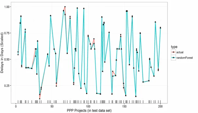
Fig. 7 shows the line plot for observed and predicted delays for linear regression (with accuracy improved by 81%). It is evident that predictions improved dramatically.

Figure 7: Evaluating observed and predicted delays in the PPP projects

5.6. Support Vector Machine (SVM)

and efficient since it used advanced optimisation algorithms to identify the best values to maximize model accuracy.

Monte-Carlo Sensitivity

PDMD 0.092

NODP 0.091

NDSC 0.087

PMDS 0.087

PLAD 0.086 FIMP 0.086 NDBW 0.085

NUSC 0.085

PSSL 0.085 IMSS 0.072 NSAI 0.066 POCI 0.053

NOD 0.010

CONTRACT 0.005

PODV 0.003

SECTOR 0.003

Listing 7: Summary of the Attributes Importance by SVM in Risk Modelling

Figure 8: Evaluating observed and predicted delays in the PPP projects

5.7 Deep Neural Network (DNN)

Figure 10: Evaluating observed and predicted delays in the

PPP projects

5.9 Comparison of Big Data Analytics Techniques

5.9.1 Comparison based on Residual Sum of Square (RSS)

modelling techniques. Further details of the results are discussed in greater detail in the next section.

Table 4: Comparison of Big Data Analytics Techniques based on RSS

Big Data Analytics

Techniques RSS

Flexibi lity

Interpreta bility

1 Random Forest 1.03 Good low

2 Decision Tree 2.17 averag

e

high

3 Linear Regression 23.20 Low high

4 Support Vector Machine 25.64 High Low

Table 5: PRAF of the Four Big Data Predictive Models and their Level of Significance (p-Value)

Sr.

#. Predictors

Ranking of Factors by Models Sum

Ran ks (∑) RA F PRA F Overa ll Ranki ng Order Linear Regression Regression Tree Random Forest Support Vector Machine Neural Network P-value Ran k Gini Ran k Impuri ty Ran k M-CSA Ran k Weig ht Ran k 1 Percentage shortage in skilled labour 0.08421 4 153.119

5

2 8.0596 6

4 0.085 9 0 0 13 0.8

1

69.1 1

1 2 Percentage Delay in Material delivery < 2e-16 1 55.2312 8 8.2713

7

3 0.092 1 0 0 19 1.1

9

54.7 5

2 3 Number of site Accidents and injuries 0.00103 2 114.301

1

5 7.2824 8

6 0.066 11 0 0 21 1.3 1

50.1 0

3 4 Percentage of design variations 0.5397 5 173.769

2

1 6.9112 1

7 0.003 15 0 0 24 1.5 0

42.9 7

4 5 Percentage of liquidated and ascertained

damages in projects

< 2e-16 1 41.3058 5

10 7.4960 8

5 0.086 5 0 0 26 1.6

3

38.2 1

5 6 Number of unforeseen site conditions 0.5938 5 132.591

4

4 6.7917 4

8 0.053 12 0 0 28 1.7 5

33.4 6

6 7 Percentage fluctuation in construction

material price index

0.00424 2 0.56240 5

16 13.600 6

2 0.005 14 0 0 29 1.8 1

31.0 8

7 8 Percent change in inflation 0.04361 3 141.694

5

3 6.4091 1

11 0.010 13 0 0 29 1.8 1

31.0 7

8 9 Average number of disputes among

parties 3.21E-06 1 62.2733 9 7 6.4906 2

10 0.085 8 0 0 30 1.8 8

28.7 1

9 10 Number of defects in a construction

project

4.48423 5 10.3091 5

15 48.883 6

1 0.003 16 0 0 30 1.8 8

28.7 0

10 11 Number of days with bad weather that

prevented site work

0.03344 3 93.3244 9

6 5.4339 5

14 0.086 6 0 0 30 1.8 8

26.3 3

11 12 Percentage of materials damaged on site < 2e-16 1 21.8976

9

14 6.5564 8

9 0.085 7 0 0 32 2.0

0

23.9 5

12 13 Number of days for site closure 0.02846 3 52.3381

7

9 6.1639 3

16 0.087 4 0 0 34 2.1 3

19.2 0

13 14 Projects were either procured via turnkey

or Design Bid Build

0.8632 5 40.0670 2

11 3.7178 8

12 0.091 2 0 0 34 2.1 3

19.1 8

14 15 Projects chosen cut across 9 sectors of the

economy

0.63428 5 36.8474 2

12 3.8068 2

15 0.072 10 0 0 37 2.3 1

12.0 7

15 16 Percentage of inferior materials supplied

to site

0.31824 5 22.0212 3

13 5.5927 3

13 0.087 3 0 0 42 2.6 3

5.9.2 Percentage Rank Factor

Going further, in order to have an overall agreement in the ranking of all predictors, the rank agreement factor (RAF) and PRAF (Elinwa and Joshua, 2001; Chan and Kumaraswamy, 2002) were applied. RAF and PRAF are mathematically computed using equation 13 and 14 respectively:

RAF=Σ(LR)(RT)(RF)(SVM)(DNN)

N 13

PRAF=RAFmax−RAFi

RAFmax

×100 %,14

Where RAFmax = maximum RAF, RAF_{i is the RAF for criteria i, N = number} of variable predictors ranked, and Σ(LR)(RT)(RF)(SVM)(DNN) = sum of the

order of rankings of Linear Regression, Regression Trees, Random Forest, Support Vector Machine and Deep Neural Network. An absolute rank difference of 2, for example, implies more agreement as to the importance of the predictor than when the absolute rank difference is 3. The rank agreement factor may be >1, with a higher factor indicating more disagreement (Elinwa and Joshua, 2001). For the 16 predictors affecting project delay, the maximum RAFmax = 2.00. A RAF of zero implies perfect agreement. The result RAF for the models is shown in the fourteenth column of Table 5. In addition, a cursory look at results of the PRAF in Table 5 shows the five most important predictors contributing to project delay to be: (1) ‘Percentage shortage in skilled labour’, (2) ‘Percentage Delay in Material delivery, (3) ‘Number of site Accidents and injuries’, (4) ‘Percentage of design variations’, and (5) ‘Percentage of liquidated and ascertained damages in projects’. These predictors are further enumerated in the discussion section.

weight (DNN). For the linear regression model, the study conducted a one-sample t-test to derive p-values for each predictor at 95% confidence level. If the mean difference is significantly different from the hypothesised value (<.05), it means that the value is statistically important in affecting project delay at the 95% confidence level (See column three and four of Table 5 for P-value of each predictor and their ranking). Going further, with regression tree, the study also evaluated the importance of some variable  when predicting   by adding up the decreases in weighted impurity for all nodes  , where  is used (averaged over all trees in the forest, but actually, we can use it on a single tree),

I(X_k)= I

M

∑

∑

N_t

N ∆ i(t) 15

Where the second sum is only on nodes   based on variable  . If   

is Gini index, then   is called Mean Decrease Gini function. In addition, in order to identify which of the predictor variables are most important for predicting project delay in PPP projects, we used random forest to derive the mean decrease impurity importance of each predictor from assemblages of randomized trees. The ranking of each predictors derived from this process are shown in column 7 and 8 of Table 5. Regarding support vector machine, sample data were smoothly segregated based on sectors and contract types. In case of DNN, hidden layers are involved with complex interactions, hence, getting a single value for attributes is not realistic. As such, zero is set as the weight and rank of these attributes in DNN to carry out the overall ranking process.

6.0 Discussion

predictive modelling of uncertainty (see also Svetnik et al., 2003). With a high error detection rate and easy identification of anomalies and outliers in data (Pal, 2017), random forest will enable automatic identification of significant predictors influencing PPP project delay (Archer and Kimes, 2008). Random forest is therefore considered a desirable technique capable of helping to make more accurate decisions toward minimizing time wastage in delivering projects.

The second phase of data analysis in this study examines the key predictors contributing towards delay in PPP projects out of the 16 predictors investigated (14 numerical and 2 categorical predictors). As evidenced in Table 5, results of PRAF calculation performed on the data relating to the 16 predictors indicate that overall, there are five most important predictors contributing towards project delay. These are: (1) ‘Percentage shortage in skilled labour’, (2) ‘Percentage Delay in Material delivery, (3) ‘Number of site Accidents and injuries’, (4) ‘Percentage of design variations’, and (5) ‘Percentage of liquidated and ascertained damages in projects’.

major impact in the industry’s completion rate , with more companies identifying insufficient skilled workers as one of the major causes of schedule overrun in projects (KPMG Global Construction Industry Report, 2015). This situation is also worsened by the insufficient number of new recruits joining the industry through apprentiship, resulting in growing skill-gap in areas such as carpenters, millwrights and electrical technicians among others (Adam et al., 2017).

(2)Percentage Delay in Material delivery – Percentage delay in material delivery was identified as the second most important predictor of project delay in this study showing a PRAF score of 54.75. Existing studies such as Van et al. (2015), Adam et al. (2017) and Ching (2014) have also highlighted the above perspective and suggested timely completion of projects is often contingent upon trouble-free supply to project site. As argued by Al-Hazim et al., (2017), the supply chain is an important stakeholder in construction project delivery and ensures the right construction material and quantities are delivered in a timely fashion at the right location. Al-Hazim et al. (2017) identified some causes of delays in material delivery as high demand for construction material, long procedure of purchasing order, poor communication between the contractor and the supplier among others ( See also Ching, 2014; Javed et al., 2013). Asides being a major cause of completion risk; delay in material delivery to site also results in significant cost overrun to the contractor in terms of wasted productive time for workers waiting for materials, penalties in liquidated and ascertained damages in the event of project’s failure to meet completion deadline etc. (Larsen et al., 2015).

emphasized construction site accidents as one of the important factors contributing to project delay. Ching (2014) suggested that unsafe behaviour is a most significant contributor to construction site accidents with a resulting impact on timely completion of projects. According to Larsen et al. (2015), in most instances of site accidents, the project manager is often obliged to either temporarily suspend site activities or in a number of fatal cases, call indefinite site closure to allow proper investigation and assessment of such accidents. This results in man-hour loss and causes disruption to schedule of projects’ activities (Van et al., 2015).

(5) Percentage of liquidated and ascertained damages in projects – The study identified percentage of liquidated and ascertained damages (LAD) as the fifth most important predictor of project delay with a PRAF value of 38.21. According to Hampton et al. (2010), liquidate and ascertained damages arises from failure of the construction contractor to successfully put the project into operations at the agreed deadline. LAD is often contractual, and the penalty for it is expressed as a financial liability to the contractor (Harty, 2005). As argued by Rebeiz (2011), except where a project contractor is a big construction firm with strong financial capabilities, a huge financial penalty in liquidated damages may cause financial distress to the contractor, which may also affect its ability to deliver the project as scheduled. As suggested by Backstrom (2013) and Javed et al. (2013) many SME contractors in the construction industry had gone bankrupt due to incurring heavy financial liabilities via liquated damages, while eventually failing to deliver such projects at their deadlines. Studies such as Adam et al. (2017), Sun and Meng (2009) argued that quick resolutions of contractual issues without recourse to lengthy court actions will mitigate the impact of LAD.

7.0 Implication for Practice:

suggesting delay as a recurring decimal within the constructi