Dynamics of magnetically driven plasma jets:
An instability of an instability, gas cloud impacts, shocks, and
other deformations
Thesis by
Auna Louise Moser
In Partial Fulfillment of the Requirements for the Degree of
Doctor of Philosophy
California Institute of Technology Pasadena, California
2012
c
2012
Acknowledgements
I would like to thank my parents Mary and Bill and my sister Alison; for their continual love and support, and for a lifetime of math and science discussions around the dinner table.
I have been fortunate enough to have many outstanding teachers. In addition to my Caltech professors, I would like to thank my high school physics teacher, George Stimson, and my undergraduate mathematics professor, Prof. Steven Agronsky. Both have legions of devoted students, and I’m pleased to count myself among them.
I would like to thank both my candidacy committee—Prof. Roy Gould, Prof. Rob Phillips, Prof. Joann Stock, and Prof. Paul Bellan—and my thesis committee—Prof. Roy Gould, Prof. Lynne Hillenbrand, Prof. Joe Shepherd, and Prof. Paul Bellan—for their insight and valuable feedback.
I have learned so much from all my groupmates, past and present: postdocs Setthivoine You and Shree-krishna Tripathi, and graduate students Steven Pracko, Gunsu Yun, Deepak Kumar, Rory Perkins, Eve Stenson, Mark Kendall, Bao Ha, Vernon Chaplin, Xiang Zhai and Zachary Tobin. I would like to give special thanks to Sett, who first taught me how to run the experiment and is always available for physics discussions and giving advice; Deepak, from whom I learned so much about the experiment and who always made me laugh; and Rory, who is both an excellent experimentalist and theorist and who entertained even my dumbest questions with patience.
Our group is also lucky to have electrical engineer Dave Felt. In addition to designing and building electronics for the lab, Dave always made time, whether it be to explain a design, to help troubleshoot a circuit, or to lend a hand in construction.
Connie Rodriguez, Eleonora Vorobieff and Christy Jenstad kept Applied Physics running smoothly; I suspect that the entire department might actually unravel without their efforts.
The assistance of Mike Gerfen in central engineering services and the accurate and quick work of Joe Haggerty and the GALCIT machine shop most certainly shortened my tenure as a graduate student, for which I am very grateful.
I would also like to thank the lunch crew: Tom, Raviv, Chris, and Matt. Lunches with them were always a highlight of my day, even if some of our ideas were better than others.
and a mostly unrelated educational background. I am so appreciative of his support, his patience, and his expertise. His constant encouragement and insight helped me to overcome my lab- and self-created obstacles. I hope that he feels that the gamble he took on me paid off.
Abstract
Contents
Acknowledgements iii
Abstract v
1 Background 1
1.1 Overview . . . 3
1.2 Magnetohydrodynamic (MHD) theory . . . 3
1.3 Force-free plasma and applications to fusion and astrophysics . . . 6
1.3.1 Woltjer–Taylor relaxation . . . 7
1.3.2 Spheromaks . . . 8
1.3.3 Jets and radio lobes as Taylor relaxed states . . . 9
1.4 Overview of experiment . . . 10
1.4.1 Apparatus . . . 10
1.4.2 Steps in plasma formation . . . 11
1.5 Laboratory astrophysics . . . 15
1.5.1 Scaling laws . . . 15
2 Instability cascade resulting in magnetic reconnection 20 2.1 Introduction to magnetic reconnection . . . 21
2.2 Exponential kink amplitude growth and Rayleigh–Taylor instability onset . . . 22
2.3 Magnetic reconnection . . . 26
2.4 Non-MHD scale . . . 32
2.5 Experiments with different plasmas . . . 35
2.6 Relevance to solar loops . . . 36
3 Collision experiments 37 3.1 Density increase and magnetic field amplification in hydrogen jets . . . 37
A.2.1 Data acquisition . . . 83
A.2.2 Fast framing camera . . . 85
A.2.3 Rogowski coil . . . 85
A.2.4 High-voltage probe . . . 85
A.2.5 R-axis magnetic probe array . . . 86
A.2.6 Spectroscopic array . . . 86
A.2.7 Interferometer . . . 86
A.2.8 Extreme ultraviolet-soft X-ray diodes . . . 86
A.2.9 Capacitively coupled probe . . . 87
A.2.10 Z-axis magnetic probe array . . . 87
A.3 Control hardware . . . 88
B Neutral gas density measurements 90 B.1 Fast ion gauge (FIG) . . . 90
B.2 Calibration process . . . 90
B.3 FIG measurements of gas distribution . . . 92
B.4 Comparison with other measurements . . . 93
B.4.1 Thermocouple vacuum gauge . . . 94
B.4.2 Paschen breakdown . . . 96
C Magnetic probe array (MPA) calibration 98
Chapter 1
Background
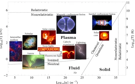
Plasma is a state of matter in which the constituent atoms are ionized: atoms are stripped of their electrons to form a fluid made up of freely moving ions and electrons. Although it is an oversimplification, we can broadly describe the states of matter according to how the atoms in each state interact. Interaction between atoms is primarily via strong chemical bonds in a solid, primarily via weak chemical bonds in a liquid, primarily via collisions in a gas, and via a combination of collisions and electromagnetic fields in a plasma. Plasmas are prevalent in nature; it is commonplace to estimate that plasma makes up about 99% of all visible matter in the universe [16, 21]. What we consider the normal states of matter—solid, liquid, and gas—are in fact quite exotic.
Because the vast majority of visible matter is in a plasma state, plasma physics underlies the dynamics of most space and astrophysical systems, from stellar dynamos to coronal mass ejections, and from super-novae to relativistic jets. In addition to distant astrophysical plasmas, familiar examples of plasmas include the auroras, lightning, and even fluorescent lights. Plasmas have applications in fusion energy, spacecraft propulsion, laboratory material processing, and the study of astrophysics.
Figure 1.1: Various plasmas and their position in density-temperature space. The dashed lines show various important transitions, calculated for hydrogen: the ionized/neutral boundary at the bottom corresponds to 1% of the hydrogen atoms being ionized (determined using the Saha equation), the classical/quantum bound-ary at the right indicates the transition to electron degeneracy (where electrons stop behaving like classical particles), the far-right relativistic/nonrelativistic boundary the transition to relativistic degeneracy, and the upper relativistic/nonrelativistic boundary corresponds tokT =mec2, but in fact electron-positron pair
temperature for a plasma, with many space plasmas being 10–100 eV and fusion plasmas being 104eV. This density-temperature information is summarized in Fig. 1.1.
1.1
Overview
Rather than a chronological arrangement, this thesis is organized to allow the reader to read about the most interesting experimental results first and to follow up on the details of the experimental hardware if desired. This introduction and background chapter provides the motivation and develops the framework and lan-guage necessary to discuss the plasma experiments. The next three chapters will present the results from three separate sets of experiments that explore different aspects of the plasma jet evolution. Chapter 2 reports a newly discovered behavior: a large-scale magnetohydrodynamic system reaching the small length scales necessary for magnetic reconnection via a series of instabilities. Chapter 3 presents results of collision experiments in which the plasma jet collides with a cloud of neutral gas, including shocks and magnetic deformation. Chapter 4 shows that straight plasma jets undergo a quasi-two-dimensional “breathing” be-havior in response to a fluctuating current amplitude. These experimental results are briefly summarized in Chapter 6.
The addition of a new power supply led to the experimental results in Chapters 2 and 4. Interested readers will find details of the new power supply design and construction in Chapter 5. (Uninterested readers may skip this chapter and proceed, unjudged, to Chapter 6.) Readers especially interested in experimental hardware may also see the appendices: Appendix A details hardware used to produce and diagnose plasmas in the Caltech experiment, Appendix B describes fast ion gauge measurements of neutral gas density, and Appendix C presents the derivation of an exact calibration matrix for the magnetic probe arrays.
1.2
Magnetohydrodynamic (MHD) theory
(a) Surfaces of constant poloidal flux (b) Contours of constant poloidal flux
Figure 1.3: Poloidal field structure in spheromaks. (a) Lines show contours of constant poloidal magnetic flux for a spheromak in a cylinder with radiusaequal to heighth. (b) Surfaces of constant poloidal flux are nested tori.
scale radio-emitting lobes.
1.3.2
Spheromaks
For a simply connected volume (that is, one topologically equivalent to a sphere, rather than a torus) with the boundary condition that no magnetic flux escapes the volume,B·ds= 0, the Taylor state is called a spheromak.
A spheromak is axisymmetric with cylindrical symmetry. Though the volume is simply connected, im-portant plasma structures within that volume are topologically equivalent to a torus. Taking advantage of the cylindrical symmetry, it is often convenient to define two directions when discussing features: toroidal, which is in theφdirection, and poloidal, which combines therandzdirections. A spheromak has a toroidal magnetic field that drops to zero at the boundary and surfaces of constant poloidal magnetic flux which are nested tori, as shown in Fig. 1.3.
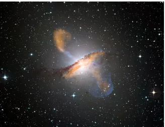
Figure 1.4: Centaurus A, an example of a galaxy with disk and associated astrophysical jets. Image is a com-posite of a visible light background overlaid with X-ray (orange) and submillimeter (blue) data. Image credit: ESO/WFI (Optical); MPIfR/ESO/APEX/A. Weiss et al. (Submillimeter); NASA/CXC/CfA/R.Kraft et al. (X-ray)
section of the jet [46, 43, 19].
K¨onigl and Choudhuri [29] proposed that these jets are an example of a free equilibrium, and force-free models continue to hold favor [42, 45]. Others have drawn comparisons between the radio lobes these jets create, jet-hollowed out cavities in the surrounding media that emit in the radio frequency, and the spheromak Taylor relaxed state [64].
1.4
Overview of experiment
The Caltech experiment produces plasmas relevant to both spheromak studies and studies of astrophysical jets. Here, magnetically driven plasma jets precede spheromak formation, and the evolution of these jet structures can give insight into the two systems.
1.4.1
Apparatus
disk and annulus electrodes (see Fig. 1.5). In addition the Caltech experiment has no flux-conserver, that is, no conducting wall bounds the volume that the plasma grows to fill. The plasma is instead bounded by closed poloidal field lines. The experiment generates a spheromak plasma that evolves in a low-background-pressure vacuum chamber, with the wall far away.
The planar electrodes and evolution into vacuum provide diagnostic access to the plasma formation region uncommon in past spheromak experiments; the electrode geometry and minimal wall-effects also make the experiment an effective platform for studying the astrophysical phenomenon described in Section 1.3.3, namely, accretion disk polar jets. As shown in Fig. 1.6, the geometry of the electrodes mimics that of an accretion disk: planar, with a radial electric field and a dipole magnetic field linking the outer disk and its center. Gas inlets in the inner and outer electrode allow the disk to act as the material source, as in accretion disk jets, and the lack of gas backfill and flux conserver means that the laboratory jet forms and propagates out into a region of lower pressure, as in the astrophysical case.
(a) (b)
Figure 1.5: Overview of the Caltech experimental apparatus. (a) Photo of the experimental apparatus, showing the stainless steel vacuum chamber in its natural habitat, with several power supplies and the Imacon fast framing camera. (b) A cut-through diagram of the experimental vacuum chamber, showing a view of the inner cathode and outer electrode mounted on one end dome. Numerous ports and windows allow diagnostic access.
1.4.2
Steps in plasma formation
A typical experiment timeline, with plasma breakdown at t = 0, is as follows: t =−10 ms, background magnetic field coil power supply fires; t = −2 ms, outer electrode fast gas valves fire; t = −1 ms, inner electrode fast gas valves fire; t ∼ −2 to t ∼ −1 µs, the main power supply applies a voltage across the electrodes;t = 0, the gas breaks down into plasma and triggers a round of diagnostics;t = 0 tot= 10–60
(a) Accretion disk geometry (b) Caltech experiment geometry
Figure 1.6: (a) Artist’s conception of magnetic field lines linking a central object and its accretion disk. Image credit: NASA/JPLCaltech/R. Hurt (SSC). (b) The Caltech experiment electrodes, image here rotated for comparison. White lines indicate the background magnetic field, gas inlets provide material. Photo credit: Dave Bullock
diagnostics to avoid problems associated with the uncertainty in time of breakdown.
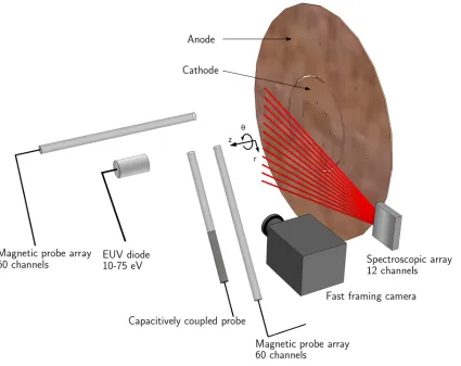
An overview of the diagnostic equipment locations and geometry is shown in Fig. 1.7. The diagnostic suite includes a fast camera; magnetic probe arrays that each measure the three-dimensional magnetic vector at twenty locations; a 12-channel spectroscopic array that can give ionization, temperature, density, and velocity data; an interferometer that gives density; extreme ultraviolet (EUV) diodes; and a capacitively coupled probe that measures electrostatic fluctuations. The z-axis magnetic probe array and capacitively coupled probe are recent additions, constructed and installed for the purposes of this thesis research. Details of diagnostic equipment are given in Appendix A.
At breakdown, the plasma forms in a radially symmetric arrangement consisting of 8 arches, one for each pair of inner and outer gas inlets, Fig. 1.8. The breakdown path is determined by the gas density according to Paschen breakdown criteria [4], and lies nearly along the imposed background magnetic field lines. The background field is locked into the plasma via flux conservation, as described in Section 1.2. The electrodes are electrically connected by these 8 current-carrying, plasma-filled flux tubes. An∼100 kA peak current flows from the outer electrode to the inner electrode; parallel currents on the inner limb of each arch compress the inner portion of the arches into a single central column as the increasing toroidal magnetic pressure between the arches and the electrodes expands the plasma loops. The result is a magnetically driven plasma with a central collimated jet structure. The magnetized plasma jet expands into the chamber at approximatelyvA=Bφ/
√
ρµ0, the poloidal magnetic field Alfv`en velocity, [34] which is∼50 km/s for a hydrogen jet.
Figure 1.7: An overview of the experiment diagnostics. (Not to scale)
(a) Detached plasma (b) Kinked plasma (c) Straight plasma
Figure 1.9: The three experimental regimes. All 3 images are from hydrogen experiments with the capacitor bank charged to 5 kV, giving a peak current ofIpeak∼90 kA. The far-left image shows a detached plasma,
Ψie = 0.54 mWb. The center image shows a kinked plasma, Ψie = 1.62 mWb. The right image shows a
straight plasma, Ψie= 2.17 mWb.
1.5
Laboratory astrophysics
By their nature, astrophysical measurements are usually remote and often static. We can rarely make direct measurements in the systems of interest and many phenomena evolve on such a long time scale that it is difficult to study their long-term dynamic evolution. By creating astrophysically relevant plasmas in a laboratory environment, we can provide an additional source of insight into astrophysical systems. This can be done both by isolating and studying physical mechanisms of general significance, and also by creating models of specific astrophysical systems in the laboratory making use of scaling laws.
1.5.1
Scaling laws
For a laboratory-scale system to model an astrophysical-scale system, there must be a congruency in the equations governing system evolution. If the dynamical systems are described by scale-independent equa-tions, equations which do not have an explicit dependence on system dimensions, then we can find scaling transformations to relate similar systems. Such scaling transformations are common in physics and engi-neering. The equations of fluid dynamics are scale-independent, which allows for the familiar examples of wind-tunnel tests of model cars and airplanes before production of full-scale vehicles. The equations of MHD are also scale-independent, allowing us to model the astrophysical systems they describe in the laboratory.
The actual ratio of magnetic field strengths isBY SO/BCIT = 3×10⁻⁶, close to the required
√
c3= 10−6, and the actual velocity ratio is vY SO/vCIT = 6, which is about an order of magnitude higher than the
requiredpc3/c2 = 0.7. Even so, considering the scale discrepancies in the two systems and the fact that many of the YSO values chosen actually come from a range of several orders of magnitude, these scaling laws are fairly well satisfied. According to the final scaling relationship,tY SO/tCIT =c1
p
Chapter 2
Instability cascade resulting in
magnetic reconnection
Magnetic reconnection is a process whereby magnetic field lines break and then reconnect to form a new topology. This process requires diffusion of field across plasma; a continuing mystery [65] is why observed reconnection rates in both space and laboratory plasmas are typically orders of magnitude faster than can be accounted for using the most obvious diffusion-enabling mechanism: classical electrical resistivity. Current thinking [13, 65] holds that the field diffusion underlying observed magnetic reconnection results from some combination of wave-particle kinetic interactions and Hall term physics that are beyond the scope of ideal MHD. These non-MHD processes become important on the ion skin depthc/ωpi or the ion Larmor radius
rLi scales, which are “microscopic” compared to the ideal MHD scale.
Shibata and Tanuma proposed that a macroscopic two-dimensional MHD system could access microscale physics via a sequence of repetitive tearing and thinning of a current sheet into two-dimensional magnetized plasma structures [60]. Relatedly, recent numerical simulations of magnetic reconnection have indicated that magnetic reconnection could involve development of fine structure over a range of scales [15]. One laboratory experiment [18] showed a transition from slow to fast magnetic reconnection when the current channels reached a microscopic scale. If these microscale non-MHD processes are indeed the enabling mechanisms for observed reconnection, the question arises: how can a macroscopic MHD system couple to the required non-MHD microscopic scales?
This chapter describes a cascade of instabilities from a distinct, macroscopic-scale MHD instability to a distinct, microscopic-scale (c/ωpi) instability associated with magnetic reconnection. The observations
2.1
Introduction to magnetic reconnection
In ideal MHD, the magnetic field is frozen-in to the plasma, which means that, as described in Section 1.2, the magnetic field lines do not diffuse across the plasma. It is a fact of nature that plasma structures and their associated magnetic fields must be able to change topology; this topology change requires that magnetic field lines break and then reconnect to form new field lines, a process called magnetic reconnection. Magnetic reconnection requires that the magnetic field lines diffuse across plasma. How can we reconcile this with the MHD model of a frozen-in field?
The microscopic details of magnetic reconnection continue to be a topic of active study. As we understand it, the plasma will continue to be well-described by the equations of ideal MHD except in a very thin layer at the location of the field reconnection. In this small region, the field must be able to diffuse across the plasma. A cartoon of the reconnection process in the case of two merging current loops is shown in Fig. 2.1.
(a) Two current loops and associated fields (b) Close-up view of region indicated by dashed line box in (a)
Figure 2.1: A cartoon of magnetic reconnection in the case of two merging current loops. (a) The current loops (red) produce magnetic field (grey lines) that must reconnect as the two loops approach each other. The reconnection happens in a very thin layer within the region indicated by the dashed line box. (b) A zoomed-in view of the reconnection region shows the thin layer in which reconnection takes place. This region is called the x-point.
The simplest diffusion-enabling mechanism is electrical resistivity, as the assumption of zero resistivity leads to frozen-in flux. In most laboratory and astrophysical plasmas, however, using the actual plasma resistivity predicts a reconnection rate orders of magnitude lower than the rates observed in these systems. Take the case of a coronal mass ejection (CME), in which material disconnects from the surface of the sun and is hurled into space. Here the resistivity is about 10−6 Ω m, which would lead to predictions of a reconnection time on the order of weeks to months for the 106 m scale. However, in observations, the reconnection in CMEs only takes seconds to minutes.
Figure 2.2: An argon plasma jet showing the three-dimensional helical structure of the kink instability. The helix is right-handed, that is, the portion of the filament on the left-hand side of the image is in the foreground, and the portion of the filament connected to the electrode on the right-hand side of the image is in the background. In this case the plasma filament shows the beginning of fine structure associated with the Rayleigh–Taylor instability. Shot #11037; image intensity is logarithmically scaled and false colored.
This method involves using a higher resistivity value than that of the actual resistivity of the plasma, which produces the desired reconnection rates but does not address the question of the small-scale processes responsible for diffusion.
Most modern theories credit a combination of small-scale processes for producing the necessary diffusion. The main processes are wave-particle kinetic interactions (plasma waves coupling to and accelerating particles to high energies) and Hall term physics or two-fluid effects (the decoupling of motion of the electrons and ions rather than electrons and ions behaving as a single conducting fluid as in MHD). Both of these processes are beyond the scope of ideal MHD and become important on the ion skin depthc/ωpi or the ion Larmor
radiusrLi scales.
2.2
Exponential kink amplitude growth and Rayleigh–Taylor
in-stability onset
(a) (b)
Figure 2.3: Kink amplitude growth rate. (a) Comparison of exponential kink growth rate and linear kink growth rate as measured from fast camera images. Circles indicate kink amplitudeξwith exponential growth
∼exp(γkinkt) withγkink= 8.3×10⁵s−1, shot #10934. Crosses indicate kink amplitude with linear growth
∼t, shot #10930. Lines show best fit to data. (b) Example of measurement of amplitudeξin shot #10934
Fig. 2.3.)
In the exponential growth case (see Fig. 2.4), a segment of the kinked jet quickly transitions to a thin filament, which then becomes very bright while developing a sharp, distinctive periodic fine structure that appears preferentially on the trailing side of the radially outward-accelerating filament. A few microseconds after this thin filament forms, it breaks up.
The growth rate, location, and spatial periodicity of this fine structure are consistent with the Rayleigh– Taylor instability in a magnetized plasma [14]. The Rayleigh–Taylor instability is a well-known pressure-driven instability that develops in a gravitational field at the interface where a heavy fluid with density ρ2 rests atop a lighter fluid with density ρ1. In the simplest, non-magnetized case, a disturbance develops at the fluid interface and as the heavy top fluid moves downward, it is replaced with upward-moving lighter fluid (Fig. 2.5). This exchange releases potential energy, as the potential energy of the light fluid due to the gravitational field is less than that of the heavy fluid it replaces. The Rayleigh–Taylor instability is an incompressible instability: the fluids are interchanged without compressing or expanding. The initially small ripple at the interface will grow exponentially in time, forming large “fingers” of interspersed material. The Rayleigh–Taylor instability is common in astrophysical situations, underlying the elongated finger-like structures visible in supernova remnants [26], as seen in Fig. 2.6.
Figure 2.4: Fast camera images of an argon plasma jet undergoing exponentially growing kink instability, developing a Rayleigh–Taylor instability and reconnecting. All images from shot #11225; image intensity is logarithmically scaled and false colored.
Figure 2.6: The Crab Nebula shows finger-like structures from Rayleigh–Taylor instabilities as the material expands outwards [26]. This is a composite image from the Hubble Space Telescope. Image credit: NASA, ESA, J. Hester and A. Loll (Arizona State University)
interface, the Rayleigh–Taylor instability will simply interchange the magnetic field lines of the two fluids if the disturbance is perpendicular to the field (k·B= 0, as described below) and will undergo an undulatory instability. Ifk·B6= 0, the disturbance is at an angle with respect to the magnetic field and the tension of the magnetic field lines stabilizes the Rayleigh–Taylor instability.
In our experiment, the acceleration of the exponentially growing kink segment constitutes the effective gravitational acceleration gef f; to an observer in the frame of the accelerating filament at the location of
the periodic structure (on the inward side of the outward accelerating filament, i.e., the trailing side), the filament would appear to be a heavy fluid sitting on top of the trailing low-density plasma immediately exterior to the filament. This is also the case for the supernova remnant; the acceleration of the exploding material provides an effective gravity that drives the Rayleigh–Taylor instabilities seen in Fig. 2.6.
The exponential growth rate of a Rayleigh–Taylor instability in a magnetized plasma is [14]
γ2=gk ρ2−ρ1 ρ2+ρ1
− 2 (k·B)
2
µ0(ρ2+ρ1)gk !
. (2.1)
The fastest growing mode of the Rayleigh–Taylor instability has k·B = 0 (where k is the instability wavevector and B is the magnetic field vector). We can see this mathematically in Eq. (2.1), where the
Figure 2.7: An argon plasma jet reconnecting after the kink instability and Rayleigh–Taylor instability. The filament in the center of the frame accelerates upward and continues to move in that direction after the filament snaps; the portion of the filament still connected to the electrode on the right-hand side of the image accelerates downward. The Rayleigh–Taylor instability is on the trailing side of both the upward and downward accelerating portions. Shot #11131; image intensity is logarithmically scaled and false colored.
the filament breakup. High-energy radiation has been shown to be associated with magnetic reconnection in the past, with solar flares producing up to GeV particles and strong X-rays [38].
A capacitively coupled probe placed in the plasma jet between the electrodes and the filament measures an order-of-magnitude increase in emissions coincident with the filament breakup (see Fig. 2.9a). We can demonstrate that the excitations are in the frequency range of whistler waves, which have been shown to be associated with magnetic reconnection [20].
Plasmas support a huge number of different types of waves, broadly broken down into two types: hot and cold plasma waves. Contrary to their names, this division is based not on the temperature of the plasma, but on whether the wave behavior is sensitive to the temperature or is independent of the temperature, respectively. We will mostly concern ourselves with waves in which the wave behavior is independent of tem-perature. For these so-called “cold” plasma waves, the plasma temperature can be set to zero in calculations without affecting the outcome.
Figure 2.8: Photodiode data show a burst of EUV radiation at the time of reconnection. The red trace, shot #11042, is from an exponentially growing kink that undergoes a Rayleigh–Taylor instability and reconnects. The red trace shows a peak in emission centered at about 30µs, the corresponding fast camera image shows fine structure at 30µs and that the plasma has reconnected by 32µs. The blue trace, shot #11044, is from a linearly growing kink, for comparison.
(a) Capactively coupled probe data (b) Fast Fourier transform of data
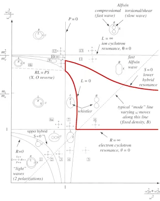
Figure 2.10: The CMA diagram is a visual representation of the wave modes sustained in a cold magnetized plasma. Boundaries between regions correspond to wave cutoff and resonances. A small Freidricks diagrams in each region shows wave front topology for the wave type in that region and the sign ofL,R,S, andP are indicated as “+” or “−” for each region. The excitations measured can be placed in the appropriate region by using known values to calculate L, R, S, P. When performed for shot #11214 this method indicates
(a) Magnetic vectors in ther−zplane, with reconnection
(b) Magnetic flux contours, with recon-nection
(c) Magnetic vectors in ther−zplane, no reconnection
(d) Magnetic flux contours, no reconnec-tion
(a) Argon plasma (b) Nitrogen plasma (c) Hydrogen plasma
Figure 2.12: Examples of Rayleigh–Taylor fine structure on top of kink-unstable plasma jets. In the case of (a) argon and (b) nitrogen plasma jets, the Rayleigh–Taylor erodes the filament to the ion skin depth or below it. The ion skin depth is 1 cm in the argon plasma and 0.5 cm in nitrogen plasma. In the case of (c) hydrogen, the diameter of the filament does not reach the ion skin depth, 0.2 cm, and we do not observe magnetic reconnection.
magnetic reconnection to occur.
2.6
Relevance to solar loops
The essential components of this mechanism have been separately observed in nature. For example, in the solar corona current-carrying magnetic flux tubes confining plasma with density higher than ambient are common, kinking of such flux tubes is also common [63, 67], and Rayleigh–Taylor instabilities have been observed [7].
Chapter 3
Collision experiments
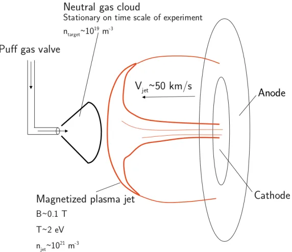
In astrophysical systems over a wide range of scales, collimated plasma jets travel at high velocity and collide with the surrounding medium. To better understand this interaction, we designed a laboratory experiment that places a localized cloud of neutral gas directly in the path of a plasma jet (Fig. 3.1) and studied the evolution of the jet-cloud system. Upon collision with the neutral cloud, the magnetized jet slows and deforms and the initially neutral cloud is ionized. The interaction is studied with several diagnostics: the fast framing camera (with and without optical filters), both ther-axis andz-axis magnetic probe arrays, and the 12-channel spectrometer. Collision experiments were performed with various combinations of hydrogen, argon, and nitrogen. The nature of the interaction depends on the plasma jet species and the neutral cloud species. There are two qualitatively different types of interaction presented in this chapter: Section 3.1 describes the evolution of a hydrogen plasma jet colliding with an argon or nitrogen neutral cloud, and Section 3.2 describes the evolution of a nitrogen or argon jet colliding with a hydrogen neutral cloud.
3.1
Density increase and magnetic field amplification in hydrogen
jets
Figure 3.1: Simplified schematic of collision experiment geometry
3.1.1
Visible interaction
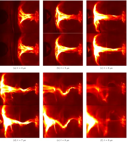
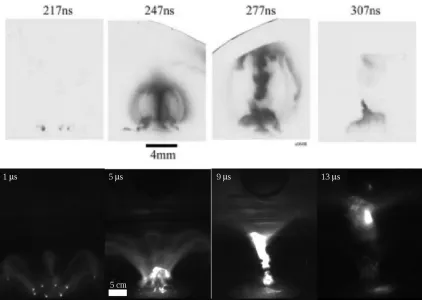
The interaction between the hydrogen plasma and the argon neutral cloud is clear in fast camera images of the collision (Fig. 3.2). The images indicate that the interaction between the plasma jet and neutral cloud starts at about 6µs after plasma breakdown, when the plasma jet has reached a length of 25 cm. The jet slows significantly, losing about 75% of its velocity. The jet front visibly thickens as the plasma collides with the neutral cloud. As shown in Fig. 3.2, the plasma appears to pile up as it collides with the neutral gas cloud.
3.1.2
Spectroscopic measurements
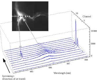
The 12-channel spectroscopic array can be used to study the interaction region in detail. The spectroscopic lines of sight are aligned along thez-axis so that they spanz= 19 cm toz= 41 cm, with the primary collision region from z = 25 cm to z = 35 cm. The spectroscopic measurement window is centered on the Balmer series H-β line at 486.13 nm and includes two argon ion (Ar II) lines at 484.78 and 487.99 nm (Fig. 3.3).
The H-βline is significantly wider due to a process known as Stark broadening. Stark broadening indicates electron density; the greater the broadening, the higher the density [66]. In Fig. 3.3, the Stark broadening indicates an electron density ne= 7.5×10²¹. The full linear array of spectroscopic measurements is shown
(a)t= 4µs (b)t= 5µs (c)t= 6µs
(d)t= 7µs (e)t= 8µs (f)t= 9µs
Figure 3.3: Spectroscopic data show Stark broadening of H-β lines and ionization of argon. Data are taken from a single channel of the 12-channel array, whose position is indicated by a red dot in the right-hand image. Measurement is centered on the H-β line at 486.13 nm. The window includes two Ar II lines at 484.78 and 487.99 nm.
the appearance of the thick front in the images and dropping off in the neutral gas region. A plot of the electron density as a function of z is shown in Fig. 3.5. These data are consistent with a picture of the plasma jet striking the initially neutral argon cloud, ionizing the argon, then slowing and piling up in the interaction region. Because the hydrogen plasma piles up when it hits the argon neutral gas, the hydrogen plasma maximum density is at lowerz than the argon neutral gas. Just past the peaking of the jet density as measured by Stark broadening is the maximum intensity of the Ar II lines.
3.1.3
Magnetic measurements
Ideal MHD theory predicts that flux is frozen-in to the plasma; a magnetized plasma will act to keep magnetic flux invariant in the frame of the moving plasma (see discussion in Section 1.2). Ideal MHD describes a plasma with a negligibly small resistivity, that is, a plasma with a large magnetic Reynolds numberRM =µ0Lv/η, where Lis the plasma length, v the velocity, andη the plasma resistivity. The thermal velocity forT = 2 eV andn∼1021 m−3 gives an ion-electron collision frequency for the hydrogen plasma jet of 7×10⁹ s−1 and an electron mean free path of lmf p ∼ 10−2 cm. The plasma resistivity is η ∼ 3×10⁻⁴ Ωm; with a
characteristic length of 25 cm and velocity of 50 km/s,, this gives a magnetic Reynolds number RM ∼50.
Because RM 1, the hydrogen jet can be treated as an ideal MHD plasma. Thus, we would expect an
increase in magnetic field to accompany an increase in plasma density. Magnetic measurements confirm that the magnetic field increases in the region of increased plasma density, consistent with this prediction.
Figure 3.4: Spectroscopic data show Stark broadening of H-βlines and ionization of argon. Traces shown are from 12-channel array, timet= 8µs with a 3µs window. Inset fast camera image is from same experiment, timet= 8µs. Stark broadening of H-β increases from low to high z; Ar II lines are brightest at highz.
(a) (b)
(c) MPA at 31 cm, in neutral gas cloud (d) MPA at 25 cm, in pile-up
(a)z= 31 cm, pile-up region. (b)z= 33 cm (c)z= 35 cm, neutral cloud region.
Figure 3.7: Magnetic data comparing an experiment with a neutral argon target (blue, shot #10551) and an experiment with no neutral target (red, shot #10533). The three plots show the total magnetic field strength on the central axis at three differentzlocations; from left to right,z= 31, 33, and 35 cm. The left-most plot corresponds to the pile-up region, the right-most to the neutral cloud region. In these experimentsVgun= 5
kV, Ψgun= 1.08 mWb.
3.1.4
Momentum analysis
We can estimate the momentum change of the jet two ways, and also measure the total jet momentum directly using a ballistic pendulum. The two estimates yield similar values and are of the same order as the independent measurement.
We can use the fast camera image of the collision experiment to estimate that at timet= 8.75µs (which we will consider the end of the collision interaction for these calculations) the lowestzvalue affected by the collision is z= 24.5 cm. This means that the jet material at lower z has not participated in the collision, and so its momentum does not need to be taken into account for this calculation. Fast camera images show that the jet has an initial velocity of∼50 km/s and that the velocity att= 8.75µs is∼17 km/s.
The first momentum calculation estimates jet volume affected by comparing a collision experiment and a non-collision experiment with the same settings. Because we know that only the jet pastz= 24.5 cm has been affected, we can estimate the volume of the jet affected by the collision by measuring the dimensions of the non-collision experiment jet at this same time. The volume estimate can then be combined with the approximate density of the unaffected jet to determine momentum change.
The non-collision jet att= 10.75µs has a length of about 38 cm, with the front about 4 cm thick and 29 cm in diameter. The jet column is approximately 7.5 cm in diameter. We are only interested in the volume of the jet pastz= 24.5 cm, which gives us a volume of
V =π(.0375)2(.38−.245−.04) +π(.145)2(.04) = 3×10⁻³ m3.
Spectroscopic measurements give a plasma density ofn∼3×10²¹m−3. Assuming that this entire volume slows to 17 km/s, this gives us a momentum change of
∆pjet=M∆v= (3×10⁻³)(3×10²¹)(1.7×10⁻²⁷)(50×103−17×103) = 5×10⁻⁴ kg m/s. (3.1)
The second momentum calculation estimates jet volume directly from the collision experiment and uses the spectroscopic measurements of density to calculate mass. We assume that all material in that volume has changed by the same velocity to calculate momentum change.
Again, only the jet material past z = 24.5 cm has been affected by the collision, and we measure the jet front to have reached z = 29.5 byt = 8.75 µs. The jet front is ∼4 cm thick and we will approximate it as a disk despite its deformation. The small length of affected column has a diameter of ∼ 7.5 cm. Stark broadening measurements (see Fig. 3.4) indicate that the density in the first 2 cm of the jet front is
(a)t= 6µs (b)t= 8µs (c)t= 10µs
(d)t= 12µs (e)t= 14µs (f)t= 16µs
Figure 3.9: Visible light images from the fast camera show the argon plasma jet front slowing only minimally as it interacts with the hydrogen neutral cloud. Top image in each set is with no neutral cloud, bottom image in each set is with a hydrogen neutral cloud. The first images show the jet fully formed but before interaction with the neutral cloud,t= 6µs. In the middle image the jet front has just encountered the neutral cloud,
t= 10µs. Bottom row images show the jet front slowed but with little to no visible thickening, final image
(a)t= 8µs (b)t= 10µs (c)t= 12µs
Figure 3.10: Visible light images overlaid with filtered light images, both from the fast camera. The overlaid images are from two different experiments with the same settings; the blue image is unfiltered visible light and the red image is light filtered with an H-αoptical filter, centered at 656.3 nm with a 1.2 nm bandwidth. These images show that the bright region ahead of the jet front is excited neutral hydrogen. Images are false-colored and intensity is scaled logarithmically for display clarity. Shot #9816 and 9818, Ψ = 1.08 mWb.
Figure 3.12: A plot showing the parameter range and results of impact experiments studying CIV effects. Red boxes show collision experiments performed at Caltech. Original figure taken from Brenning, 1992 [12]
Nevertheless, the theory has proven fairly robust, with the effect identified in experiments over a wide range of magnetic field strengths and particle densities [12, 36]. More recent refinements to the theory attempt to address the energy transfer mechanism. Forerunners include the lower hybrid instabilities [36], specifically the modified two-stream instability [52, 59]. The requirements for the modified two-stream instability as a mechanism predict an effective range for the CIV interaction [11] shown in Fig. 3.13. As the critical ionization effect continues to be important in space applications, as well as in any laboratory experiment in which neutrals and plasmas interact, a greater understanding of the effect is desirable. Past experiments yielded mixed results, with laboratory experiments often seeing a CIV effect and space experiments rarely seeing a CIV effect [12, 36].
The interaction of the plasma jet and neutral cloud can be cast as a CIV interaction. As is required for a CIV effect, there is a magnetic field component perpendicular to the relative velocity of the neutral and plasma at the jet front, in this case Br. The magnetic field moves with the plasma; hence, in the plasma
frame, the neutral gas is moving into the stationary magnetized plasma at the jet velocity. In hydrogen jet/argon neutral cloud experiments the jet velocity of∼50 km/s is much faster than the critical velocity of argon, vc = 8.7 km/s. In argon jet/hydrogen neutral cloud experiments the jet velocity of∼20 km/s is
slower than the critical velocity of hydrogen,vc = 50.9 km/s. The jet interaction with the neutral cloud is
Figure 3.13: A proposed mechanism for CIV produces bounds on when the effect should be present. (a) Blue-shaded area represents the velocity range in which the CIV effect should be seen, as a function of magnetic field strength. The lower limit is the critical ionization velocity and the upper limit is v =vA
√
1 +β, the velocity at which electromagnetic modes are excited [11]. Tan-shaded region is the velocity range in the Caltech experiment. Values are determined for an argon neutral gas and a hydrogen plasma with density
ne= 1021m−3and temperaturet= 2 eV. (b) Blue-shaded area represents the plasma density range in which
the CIV effect should be seen, as a function of magnetic field strength. The plotted range is determined by p
me/mn< ωpe/ωce< c/v
p
(1 +β)me/mi. The upper velocity limit from (a) gives the upper limit for the
density and the lower limit is set by the requirement that growth rate of the instability be much greater thanωci[11]. Tan-shaded region is the density range in the Caltech experiment.
3.4
Relevance to astrophysical jets
Chapter 4
Breathing mode and two-dimensional
behavior
This chapter describes a behavior seen in the jet experiment after the addition of the pulse forming network (PFN) power supply described in Chapter 5. Using the short duration power supply for plasma breakdown and the PFN for sustainment generates a current trace that fluctuates several times over the course of the experiment (see Fig. 4.1, and see Section 5.5 for more about the PFN current). This current fluctuation means a fluctuation in the toroidal magnetic field, which relates to the jet radius. By studying the nature of the changes in the jet we see that the jet behaves quasi-two-dimensionally.
4.1
Observations of jet and current channel radius
The magnetically driven plasma jet generated by the Caltech experiment can be unstable to the current-driven kink instability described in Section 1.4.2. The factor that determines jet stability isα=µ0I/Ψ; the jet is kink-unstable whenα >4π/`. We can see from the form ofαthat a larger magnetic flux Ψ will make the jet more stable. The magnetic flux Ψ is the integral of the applied background magnetic field over the area of the inner electrode; hence, a large applied field makes the jet more stable against kinking.
The longer duration of the PFN current pulse produces physically longer jets than the short-duration power supply. Because the plasma jet stability also depends on the jet length`, approaching instability as
`increases, the background magnetic field must be fairly strong to keep the longer jet in the stable regime. The stronger background magnetic field helps keep the jet stable both by keeping Ψ large and by keeping`
smaller: to expand inz the jet must fight against the tension of the magnetic field lines, and so it travels at a slightly lower velocity than lower background magnetic field plasma jets.
Figure 4.1: The current fluctuates over the course of a high bias magnetic field experiment with the PFN and capacitor bank. Shot #11200; corresponds to fast camera image in Fig. 4.2 below.
This effect is visible in both fast camera images and in current measurements.
Fast camera images show that, in early times, straight argon plasma jets resemble those generated using the short-time-duration power supply. Once fully formed, the radius of the column viewed in fast camera images expands, contracts, and expands again in a “breathing” manner, as seen in Fig. 4.2.
The plasma jet is a current-carrying plasma-filled flux tube, but the visible jet does not necessarily coincide exactly with the region through which the electrical current flows, called the current channel. For example, we know from previous experiments that the current channel in hydrogen plasmas has a larger diameter than the visible plasma jet, extending out to a ∼ 10 cm radius for a plasma jet, with a visible radius of∼3 cm as measured from fast camera images [35].
We can measure the current channel as a function of time to verify the apparent “breathing” behavior. The current channel radius is calculated using data from ther-axis magnetic probe array (MPA). For a jet with cylindrical symmetry (i.e., not kinked), we measureBθand calculate the current enclosed at that radius
using Ampere’s law
I
C
B·dl=µ0Ienclosed
Z 2π 0
Bθr dθ=µ0Ienclosed
Ienclosed(r) =
µ0 2πrBθ
.
We plot the current enclosed at each radial measurement location at a specified time, and then determine the current channel radius as the r position at which the current has reached a certain fraction for the peak current value measured in the channel 0.65Ipeak (see Fig. 4.3). It is worth noting that in these argon
Figure 4.2: Fast camera images showing the plasma “breathing” with the fluctuating current. Images shown range fromt= 16µs tot= 37µs. Shot #11200
(a) Camera image showing jet diameter (b) Enclosed current atz= 14 cm,t= 30µs
Figure 4.3: Fast camera image of plasma jet indicating diameter and current channel measurement. (a) An argon jet at 30 µs after plasma breakdown. The arrows indicate the diameter at the z location of the r
axis MPA, which measures the current channel. Radius estimated from the camera image isr∼6 cm. (b) Plot of the current enclosed within the jet as a function of radius, calculated fromBθ as described in the
text. The enclosed current increases as a function ofr in the jet and then levels off at the peak value once outside the jet (the return current is outside the measured radius). The radius of the current channel is
r= 0.65Ipeak∼7 cm. Note that the peak enclosed current measured is∼62 kA, while the current measured
channel calculated from magnetic data, unlike hydrogen jets for which the current channel is significantly larger.
The time-changing current channel radius was measured at several zlocations along the jet length, and the results are shown in Fig. 4.4. Current values are plotted for each time at which current channel radius was measured, allowing us to compare the fluctuations of the current in time with fluctuations in the current channel radius with time. Close to the electrodes, at a low z value, the radius of the current channel is inversely proportional to the current amplitude (Fig. 4.4a). The current starts high and the current channel radius low; then as the current drops the radius increases, reaching a peak radius at approximately the same time that the current amplitude reaches a minimum. The current channel radius then drops to a minimum at approximately the same time that the current amplitude reaches its second and final peak.
Measurements of current channel radius taken farther from the electrodes, at higher z, show a similar fluctuating form, but offset in time, so that the peak current channel radius occurs later than the minimum current amplitude (Fig. 4.4b). Taken together, the measurements of current channel radius at various z
positions show the column expansion and contraction, as well as propagation of the disturbance up the jet, from electrode (lowz) to jet front (highz). Comparing the time of the peak value in the three measurement curves, we estimate that the disturbance propagates at approximately 19 km/s. By noting that the jet front reaches the magnetic probe array position at z = 28.5 cm in about t = 19 µs, we measure an average jet velocity of approximately 15 km/s.
Rather than the radius of the entire jet fluctuating together in response to the changing current (and hence magnetic field), the disturbance propagates up the column at approximately the jet velocity, the toroidal field Alfv´en velocity. The jet response to the current change does not happen simultaneously as might be expected; rather the jet responds closer to the electrodes and then the information propagates in
z with the jet.
This behavior may be of interest for laboratory plasma experiments in which collimated flows are impor-tant [61, 37]. If the flows are magnetically driven, our observations suggest that any changes in the magnetic field driving the flow would take time to propagate up the flow, rather than taking effect throughout the flow immediately.
4.2
Balancing pressure: The Bennett relation
Figure 4.5: The current radius at z= 14 cm as a function of current. The data are shown with aγ= 2 fit (2D, solid line), aγ= 5/3 fit (3D, dotted line), andγ= 2.4 fit (best fit to data, dashed line).
If the plasma is compressible and volume compresses only in the radial direction, then the number of particles per length (and hence the`of ourNparticles under consideration) remains constant. For a constant
`, Eq. (4.2) simplifies to
I2∼r2(1−γ)`−γ
∼r2(1−γ)
=⇒ r∼I1/(1−γ). (4.3)
We would usually useγ= 5/3 for a monatomic ideal gas; however in this case, we have to be careful when determining the value ofγ. We know thatγ= (m+ 2)/m, wheremis the degrees of freedom of the system. We have a monatomic gas, so there are no contributions from either rotation or vibration, and the degrees of freedom are simply the dimensionality of the system. Because we are assuming that the compression happens only radially and not along the length, compression is two-dimensional. This requires thatγ= (2 + 2)/2 = 2 to be consistent with our assumption of constant length. So in this case,ras a function ofI is:
r∼I1/(1−γ)=I−1. (4.4)
We can plot the current channel radius as a function of current at the positionz= 14 cm (see Fig. 4.5). Figure 4.5 shows the fit to the data for Eq. (4.4) withγ= 2 for the two-dimensional compression case. The plot includes the fit using γ = 5/3, as well as the best fit, r∼I−0.7, which corresponds to γ = 2.4. The
two-dimensional process.
4.3
Relevance to astrophysical jets
Chapter 5
Pulse forming network power supply
A pulse forming network (PFN) is a capacitor bank power supply that uses inductors and capacitors in parallel to produce a square voltage pulse. Experiments with the older short-duration power supply produce a plasma jet that exhibits a range of behaviors determined by current-driven instabilities, but the length of the current pulse limits the time duration of the experiment, as the current drops rapidly post-instability-onset. The PFN was designed to provide a current ∼5 times longer than that previously provided to the plasma experiment, allowing us to study the plasma column post-instability-onset.
5.1
Theory of operation
The pulse forming network design is based on transmission line theory. A transmission line can be modeled as an arrangement of discrete capacitors and inductors. A PFN uses this model to take advantage of transmission line properties (compare Fig. 5.1 and Fig. 5.2); inductors and capacitors produce a square voltage pulse with a height of half the charging voltage and a duration of twice the individual segmentLC
rise time multiplied by the number of segments.
5.1.1
Review of transmission lines
We begin with a review of transmission line theory, using a coaxial transmission line as an example. A coaxial transmission line, with in inner conductor of radius a and an outer conductor at radiusb, can be thought of as a long cylindrical capacitor with inductance. The transmission line has capacitance per length
C0 and inductance per lengthL0 given by:
C0= 2π0
ln ab, L 0= µ0
2πln
b
a
Figure 5.2: Circuit diagram of a pulse forming network with N capacitor, inductors, and resistors. In this diagram, theNth inductor and resister correspond to the plasma, and so are labeled with a subscriptp.
forj= 1 toj=N−1. This can be rewritten
Qj
Cj
−Qj+1
Cj+1
=IjRj+Lj
dIj
dt . (5.14)
For the last section,j =N, which includes the plasma modeled here as a resistor (RP) and inductor (LP)
in series, the corresponding equation is
QN
CN
=IPRP+LP
dIP
dt . (5.15)
The current through the first resistor, I1 satisfies
dQ1
dt =I1 (5.16)
and the current through thejth resistor (forj = 2 toj=N−1) satisfies
dQj
dt =Ij−1−Ij. (5.17)
The current through the plasma,Ip, satisfies
dQN
dt =IN−1−Ip. (5.18)
Figure 5.3: The numerical solution of Eqs. (5.14)–(5.18) for a 10 section PFN. PFN values used areC= 120
µF,L= 0.3µH,R= 0.3 mΩ, with a charging voltage of 4 kV. Load resistance is matched to PFN impedance,
R=pL/C = 42 mΩ. Note that the voltage pulse is approximately half the charging voltage and that the length is approximately 2×10×τ= 120 µs, whereτ=√LC = 6µs.
5.2
Design and construction
Known plasma parameters, a desired output voltage of 2–2.5 kV, and the availability of voltage, high-current capacitors dictated PFN design details. Our plasma jets draw a high-current ofI∼100 kA for a voltage of V = 2–2.5 kV. The capacitors used are Maxwell Laboratories, Inc., castor oil capacitors with C = 120
µF, an effective series inductanceL= 0.03µH, a 10 kV maximum charging voltage, and 100 kA maximum current. To keep the current output safely under the capacitor current limit, the final PFN design uses 2 identical 5-capacitor segments arranged in parallel (Fig. 5.5).
Design parameters were based on two criteria, each discussed in detail below: impedance matching between the PFN and the plasma load, and a desired rise time of∼5 µs. For optimal power delivery and an output voltage of half the charging voltage, the PFN should be impedance-matched to the plasma load. The nominal plasma impedance is∼25 mΩ; experiments have shown that while the plasma has a resistance of ∼ 2.5 mΩ, the entire circuit, including cables and ignitron, has an impedance of ∼ 60 mΩ [35]. The PFN was designed to drive a load of approximately 25 mΩ; because it is composed of two parallel segments, this means a segment impedance of 50 mΩ. Transmission line theory gives a characteristic impedance of
Z=pL/C, so the 50 mΩ requirement and 120µF capacitors indicate a section inductance of
Figure 5.4: Diagram of the inductor geometry. The sketch shows a top-down view of two capacitors connected by a single inductor. The inductor is made of three independent pieces of silver-coated copper busbar. The two vertical bars in the sketch are bolted to the center pin of their respective capacitors. The cross bar can be bolted in place across the two vertical bars in 4 possible positions, each giving a slightly different inductance.
capacitors haveC= 120µF, so a desired τ∼5µs requires a section inductance of
L=τ 2
C =
(5µs)2
120µF= 0.21µH. (5.20)
These two criteria, impedance matching (Eq. (5.19)) and rise time (Eq. (5.20)), indicate a section inductance of L= 0.2–0.3 µH. This is a small inductance; a length of wire generally has an inductance of
∼µH. Metal straps are commonly used in applications requiring low inductances. The inductor choice was based on the need to ensure that the straps used to construct the inductors have a resistance that is small compared to the PFN impedance, Z =pL/C/2 = 20–25 mΩ. Resistance depends on skin depth, so our material choice requires analysis of skin depth at the two relevant timescales: the section rise time and the PFN pulse length. The skin depth is δ = 2pηt/µ0 for a time t and material electrical resistivity η. For copper, which has an electrical resistivity ofη = 1.7×10⁻⁸ Ω m, the skin depths areδ= 5.2×10⁻⁴m for a timescale of 5µs and δ= 1.6×10⁻³ m for a timescale of 50µs. The strap thickness will be of the same order as the skin depth. A width of 1 inch is standard for straps, and we know that the capacitors have a width of 8 inches. With turns, the inductor straps will be approximately a factor of two larger than this 8 inch width. This will give an approximate resistance of
R= ηl
wδ ∼
(1.7×10⁻⁸)(0.4)
(.025)(1.6×10⁻³) = 0.2 mΩ
Figure 5.7: Sketch of one section of the dummy load. Top image is a top-down view of one section of the dummy load (approximately to scale), bottom image is side view (not to scale). Three additional sections would be attached in parallel to this one along the copper ribbon at right.
gaps with RTV 102 cement. Breakdowns were not eliminated entirely, because we could not fill the gaps between electrode and Kapton in the region where bolts connect the copper to steel. This kept us from testing the PFN on the dummy load at charging voltages over 4.25 kV. Nonetheless, the dummy load tests proved sufficient.
A voltage trace of PFN discharge through the dummy load is shown in Fig. 5.8. For a charging voltage of 4 kV, the voltage is slightly less than 2 kV: half the charging voltage, as expected. The slight drops in voltage at about 20µs and 30µs indicate dielectric barrier discharge activity. There were visible reflections of the pulse due to imperfect impedance matching between the PFN and dummy load, giving the falling side of the voltage trace a step-like appearance.
5.4
PFN-only experiments
The PFN was incorporated into the experiment in stages. First we attached the PFN cables across the electrodes and looked for interactions when generating a plasma using only the old power supply. When the connection produced no visible effect, we tried using the PFN only to break down the plasma, starting at low charging voltages. We gradually increased the charging voltage until we were making plasmas with the PFN at a charging voltage ofV = 4 kV. The current trace is smoother than that expected from theory, using a constantLandR, Fig. 5.9.
(a) The dummy load (b) Voltage trace for the PFN across the dummy load
Figure 5.8: A dummy load was designed to mimic the plasma for PFN tests. Photograph on the left is of the dummy load, attached to the PFN using the cables and clamps with which the PFN would later be attached to the experiment electrodes. Trace on the right shows the voltage across the dummy load for a PFN charging voltage of 4 kV. The voltage is slightly less than the expected 2 kV, and a reflection is visible after the primary voltage pulse. The drops in voltage seen at 20µs, 28 µs, and 38µs are dielectric barrier discharge activity.
Figure 5.9: A comparison of the experimental current trace and the numerical solution. The experimental current trace (red trace) is for a charging voltage of 4 kV. The numerical solution (blue trace) uses two parallel segments of 5 capacitors each, as described in the next section. PFN valuesC = 120 µF,L= 0.3
µH, R = 0.3 mΩ, and a charging voltage of 4 kV, for plasma parameters Lp = 265 nH and Rp = 62.5
(a) Hydrogen plasma jet produced with short-duration power supply
(b) Hydrogen plasma jet produced with PFN only
Figure 5.10: Comparison between hydrogen jet made with short-duration power supply (top) and with PFN only (bottom)
more detailed discussion of how a fluctuating current amplitude can affect the column width, see discussion in Chapter 4.
5.5
Experiments with both power supplies
(a) Line-integrated density (b) Current
(a) Short-duration power supply (b) Pulse-forming network
(c) Both power supplies together
Figure 5.12: Current traces of various power supply configurations. Each plot shows a single configuration current trace in red, and with the other two configurations shown in light gray for comparison. (a) Short-duration capacitor bank power supply current trace (shot #8908), (b) long-Short-duration PFN power supply current trace (shot #10085), and (c) both power supplies used together (shot #10801). All current traces are from hydrogen experiments with power supply charging voltagesVCB = 5 kV andVP F N = 4 kV, and a
bias field setting ofVbias= 200 V.
supply current has dropped to zero. We therefore get the fast rise time of the short-duration power supply, and the longer time duration of the PFN. The combined power supply current pulse has a FWHM of∼60
µs, about 6 times the length of the current pulse from the short-duration power supply.
The extended current duration allowed us to see several new plasma behaviors. Most significantly, it allowed us to identify the instability cascade leading to magnetic reconnection described in Chapter 2. In addition we observed the behavior of the straight jet radius in response to a fluctuating current amplitude, the “breathing” behavior described in Chapter 4. Also observed for the first time after addition of the PFN was a kink-unstable plasma jet with two twists, as described in the next section.
5.6
Kink instability with two twists
short-(a) Hydrogen, PFN only (b) Argon, both power supplies
Figure 5.13: Fast camera images showing double-twist kink plasma jets. (a) A hydrogen jet formed using the PFN only. Two twists appear simultaneously. (b) Argon jets formed using both power supplies. One twist forms and moves with the jet away from the electrodes; a second smaller radius twist forms later, closer to the electrodes. Argon jets with two twists develop Rayleigh–Taylor instabilities later in time (the beginnings of Rayleigh–Taylor fine structure is visible in both cases argon jets shown here).
duration capacitor bank (see Fig. 5.13a). In argon plasma the two twists were seen with the short-duration capacitor bank for breakdown and the PFN for sustainment (see Fig. 5.13b). It should be noted that no experiments using only the PFN have been performed with argon, and relatively few have been performed using both power supplies with hydrogen. No double twists have been observed in nitrogen thus far, but many fewer nitrogen experiments have been performed than hydrogen or argon experiments.
In the hydrogen case, the plasma column becomes kink-unstable and the two twists appear simultaneously. In contrast, in most cases the argon plasma column appears to become kink-unstable and develop one twist. A second twist appears near the electrode at low zat a later time as the first twist translates in z. In only one argon double-twist example do the two twists appear to onset simultaneously, as in the hydrogen case. All double twists observed in argon experiments precede Rayleigh–Taylor instability formation (see Chapter 2 for more details on Rayleigh–Taylor instabilities).
Chapter 6
Summary
This thesis reported the results of three sets of plasma experiments performed with the Caltech sphero-mak experimental apparatus. The three distinct topics are united as variations on a similar theme: the deformation of magnetically driven collimated plasma jets.
The magnetic reconnection experiments discussed in Chapter 2 demonstrate a new and unexpected behavior: the ideal MHD plasma undergoes a current-driven kink instability which then drives a finer-scale Rayleigh–Taylor instability. When growth of the Rayleigh–Taylor instability thins the plasma column to the necessary “microscopic” length scale, the plasma undergoes magnetic reconnection. Fast camera images clearly show the large-scale helical plasma jet developing the periodic fine-scale structure of the Rayleigh– Taylor instability, and show the plasma column breaking after Rayleigh–Taylor growth. The topology change of the magnetized structure indicates magnetic reconnection, and is accompanied by additional signatures of reconnection. This three-dimensional cascade of instabilities links the large scale of an MHD plasma system and the comparatively microscopic scale of the magnetic reconnection process, allowing the ideal MHD system to undergo reconnection. Magnetic reconnection underlies the dynamical evolution of plasma systems from tokamak fusion experiments to solar coronal loops, and the way in which large-scale MHD plasmas bridge the gap in length scales to access the microscale physics has been a topic of study for years. These results demonstrate one possible process by which this can be accomplished.
wave is produced. An argon jet colliding with a hydrogen neutral gas cloud will also slow, but not enough to produce an observable pile-up. Instead, the argon jet acts like a piston, launching a shock wave into the hydrogen neutral cloud.
Use of a short-duration power supply for plasma breakdown together with a long-duration power supply for plasma sustainment supplies the experiment with a current whose amplitude fluctuates in time. Chapter 4 shows that this fluctuating amplitude causes a “breathing” mode in a straight plasma jet: the plasma column expands and contracts radially, and this disturbance travels along the jet. The radius is found to scale with current amplitude asr∼I−1, consistent with an assumption of two-dimensional compression.
Appendix A
Caltech experimental apparatus
A brief overview of the experimental apparatus and diagnostic tools was given in Section 1.4. This appendix gives a more detailed description of plasma generation and diagnostic hardware that is helpful, but not strictly necessary, for understanding the work presented in this thesis. This includes equipment newly constructed and installed as part of this thesis research: the pulse forming network (PFN) power supply, the z-axis magnetic probe array, and the capacitively coupled probe.
A.1
Plasma generation hardware
The Caltech spheromak formation experiment uses a novel, coplanar, concentric electrode arrangement that enables direct observations of the early steps in the spheromak formation process, and matches accretion disk boundary conditions. The electrodes are 1/4-inch-thick copper, the cathode a 20.3-cm-diameter disk, and the anode a 50.8-cm-diameter annulus (see Fig. A.1). The anode is at chamber ground, and a ceramic break at the cathode mounting point isolates the cathode from ground. The two electrodes are separated by a 6.35 mm gap, but no electric breakdown occurs in this gap, as there is not enough gas density to satisfy the Paschen breakdown criteria [4]. The electrodes are mounted on one end of a 1.48-m-diameter, 1.58-m-long, cylindrical stainless steel vacuum chamber, as shown in Fig. A.1. The dimensions of the chamber are such that the∼25 cm plasma evolves with minimal wall interactions.

![Figure 2.6: The Crab Nebula shows finger-like structures from Rayleigh–Taylor instabilities as the materialexpands outwards [26]](https://thumb-us.123doks.com/thumbv2/123dok_us/1056159.1131915/33.612.203.492.76.290/figure-nebula-nger-structures-rayleigh-instabilities-materialexpands-outwards.webp)