Japanese Sentiment Classification with Stacked Denoising Auto-Encoder
using Distributed Word Representation
Peinan Zhang
Graduate School of System Design Tokyo Metropolitan University [email protected]
Mamoru Komachi
Graduate School of System Design Tokyo Metropolitan University
Abstract
Traditional sentiment classification methods often require polarity dictionaries or crafted features to utilize machine learning. How-ever, those approaches incur high costs in the making of dictionaries and/or features, which hinder generalization of tasks. Ex-amples of these approaches include an ap-proach that uses a polarity dictionary that can-not handle unknown or newly invented words and another approach that uses a complex model with 13 types of feature templates. We propose a novel high performance sentiment classification method with stacked denoising auto-encoders that uses distributed word rep-resentation instead of building dictionaries or utilizing engineering features. The results of experiments conducted indicate that our model achieves state-of-the-art performance in Japanese sentiment classification tasks.
1 Introduction
As the popularity of social media continues to rise, serious attention is being given to review informa-tion nowadays. Reviews with positive/negative rat-ings, in particular, help (potential) customers with product comparisons and to make purchasing deci-sions. Consequently, automatic classification of the polarities (such as positive and negative) of reviews is extremely important.
Traditional approaches to sentiment analysis uti-lize polarity dictionaries or classification rules. Al-though these approaches are fairly accurate, they depend on languages that may require significant amounts of manual labor. Further, dictionary-based methods have difficulty dealing with new or un-known words.
Machine learning-based methods are widely adopted in sentiment classification in order to miti-gate the problems associated with the making of dic-tionaries and/or rules. One of the most basic features used in machine learning-based sentiment classifi-cation is the bag-of-words feature (Wang and Man-ning, 2012; Pang et al., 2002). In machine learning-based frameworks, the weights of words are auto-matically learned from a training corpus instead of being manually assigned.
However, the bag-of-words feature cannot take syntactic structures into account. This leads to mis-takes such as “a great design but inconvenient” and “inconvenient but a great design” being deemed to have the same meaning, even though their nu-ances are different; the former is somewhat nega-tive whereas the latter is slightly posinega-tive. To solve this syntactic problem, Nakagawa et al. (2010) pro-posed a sentiment analysis model that used depen-dency trees with polarities assigned to their subtrees. However, their proposed model requires specialized knowledge to design complicated feature templates. In this study, we propose an approach that uses distributed word representation to overcome the first problem and deep neural networks to alleviate the second problem. The former is an unsupervised method capable of representing a word s meaning without using hand-tagged resources such as a po-larity dictionary. In addition, it is robust to the data sparseness problem. The latter is a highly expressive model that does not utilize complex engineering fea-tures or models.
• We show that distributed word representation learned from a large-scale corpus and multi-ple layers (more than three layers) contributes significantly to classification accuracy in senti-ment classification tasks.
• We achieve state-of-the-art performance in Japanese sentiment classification tasks without designing complex features and models.
2 Related Works
In this section, we discuss related works from two areas: sentiment classification and deep learn-ing (distributed word representation and multi-layer neural networks).
2.1 Sentiment classification
Sentiment classification has been researched ex-tensively in the past decade. Most of the previ-ous approaches in this area rely on either time-consuming hand-tagged dictionaries or knowledge-intensive complex models.
Ikeda et al. (2008) proposed a method that clas-sifies polarities by learning them within a window around a word. Their proposed method works well with words registered in a dictionary. However, building a polarity dictionary is expensive and their approach is not able to cope with unknown words. In contrast, our proposed approach does not use a po-larity dictionary and works robustly even when there are infrequent words in the test data.
In a similar manner, Choi et al. (2008) proposed a method in which rules are manually built up and po-larities are classified considering dependency struc-tures. However, the rules are based on English, which cannot be applied directly to other languages. This is unlike our method, which does not employ any language-specific rules.
Nakagawa et al. (2010) proposed a supervised model that uses a dependency tree with polarity as-signed to each subtree as hidden variables. The pro-posed approach further classifies sentiment polari-ties in English and Japanese sentences with Condi-tional Random Field (CRF), considering the interac-tions between the hidden variables. The dependency information enables them to take syntactic structures into account in order to model polarity flip. How-ever, their proposed method is so complex that it has
to create multiple feature templates. In contrast, our model is quite simple and does not require the engi-neering of such features.
2.2 Deep learning
One of the great advantages of deep learning is that it reduces the need to hand-design features. In-stead, it automatically extracts hierarchical features and enhances the end-to-end classification perfor-mance learned through backpropagation. As a con-sequence, it avoids the engineering of task-specific ad-hoc features using copious amounts of prior knowledge. Further, it sometimes surpasses human-level performance (He et al., 2015). Two of the most actively studied areas in deep learning for NLP ap-plications are representation learning and deep neu-ral networks.
Representation learning Several studies have at-tempted to model natural language texts using deep architectures. Distributed word representations, or word embeddings, represent words as vectors. Dis-tributed representations of word vectors are not sparse but dense vectors that can express the mean-ing of words. Sentiment classification tasks are sig-nificantly influenced by the data sparseness prob-lem. As a result, distributed word representation is more suitable than traditional 1-of-K representation, which only treats words as symbols.
In our proposed method, to learn the word embed-dings, we employ a state-of-the-art word embedding technique called word2vec (Mikolov et al., 2013b; Mikolov et al., 2013a), which we discuss in Sec-tion 3.1. Although several word embedding tech-niques currently exist (Collobert and Weston, 2008; Pennington et al., 2014), word2vec is one of the most computationally efficient and is considered to be state-of-the-art. Collobert et al. (2008) presented a model that learns word embedding by jointly per-forming multi-task learning using a deep convolu-tional architecture. Their method is considered to be state-of-the-art as well, but it is not readily applica-ble to Japanese.
adds high generalization ability to auto-encoders. This method is used in speech recognition (Dahl et al., 2011), image processing (Xie et al., 2012) and domain adaptation (Chen et al., 2012); further, it ex-hibits high representation ability.
Glorot et al. (2011) used SdAs to perform domain adaptation in sentiment analysis. After learning sen-timent classification in four domains of the reviews of products on Amazon, they tested each model with different domains. Although the task and method are similar to those of our proposed approach, they only use the most frequent verbs as input.
Dos Santos et al. (2014) and Tang et al. (2014) researched sentiment classification of microblogs such as Twitter using the distributed representation learned by the methods of Collobert et al. (2008) and Mikolov et al. (2013b; 2013a). Those two tasks are the same task as ours, but the former generats sentence vectors using string-based convolution net-works while the latter utilizes a model that treats the distributed word representation itself as polari-ties. Our proposed approach makes sentence vectors by simply averaging the distributed word represen-tation, yet achieves state-of-the-art performance in Japanese sentiment classification tasks.
Kim (2014) classified the polarities of sentences using convolutional neural networks. He built a sim-ple CNN with one layer of convolution, whereas our model uses multiple hidden layers.
Socher et al. (2011; 2013) placed common auto-encoders recursively (recursive neural networks) and concatenated input vectors to take syntactic in-formation such as the order of words into account. In addition, they arranged auto-encoders (AEs) to syn-tactic trees to represent the polarities of each phrase. Recursive neural networks construct sentence vec-tors differently from our approach. Compared to their model, our distributed sentence representation is quite simple yet effective for Japanese sentiment classification.
3 Sentiment Classification with Stacked Denoising Auto-Encoder using
Distributed Word Representation
In this study, we treated the task of classifying the polarity of a sentence as a binary classification.
Our proposed approach makes a sentence vector from the input sentence, and then inputs the
sen-tence vector to a classifier. The sensen-tence vector is computed from the average of word vectors in the sentence, based on distributed word representation.
In Section 3.1 we introduce distributed represen-tation of words and sentences, and in Section 3.2 we explain multi-layer neural networks.
3.1 Distributed representation
1-of-K representation is a traditional word vector representation for making bag-of-words. The di-mension of a word vector in 1-of-K is the same as the size of the vocabulary, and the elements of a dimension correspond to words. 1-of-K treats dif-ferent words as discrete symbols. However, 1-of-K representation fails to model the shared meanings of words. For example, the word vectors “dog” and “cat” should share “animal” or “pet” meanings to a certain degree, but 1-of-K representation is not able to capture this similarity. Consequently, we propose distributed word representation.
The task of learning distributed representation is called representation learning and has been of sig-nificant interest in the NLP literature in the last few years. Distributed word representation learns a low-dimension dense vector for a word from a large-scale text corpus to capture the word’s features from its context.
3.1.1 Distributed word representation
Let the number of vocabularies be|V|, the dimen-sion of a vector representing words bed, 1-of-K vec-tor beb ∈ R|V| and the matrix of all word vectors be L ∈ Rd×|V|. Thekth target word vectorwk is consequently represented as in Equation 1.
wk=Lbk (1)
Continuous Bag-of-Words (CBOW) and Skip-gram models in word2vec (Mikolov et al., 2013b; Mikolov et al., 2013a) have attracted tremendous attention as a result of their effectiveness and effi-ciency. The former is a model that predicts the tar-get word using contexts around the word, whereas the latter is a model that predicts the surround-ing context from the target word. According to Mikolov’s work, skip-gram shows higher accuracy than CBOW1. Therefore, we used skip-gram in our experiments.
1
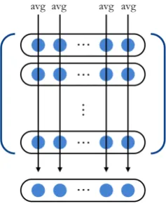
outper-Figure 1: The sentence vector construction method.
3.1.2 Distributed sentence representation
In our approach, we construct a sentence matrix S ∈ R|M|×d from the corpus containing |M| sen-tences.
First, we describe how to create a sentence vector from word vectors. The ith (1 ≤ i ≤ M) input sentence composed of|N(i)|words is used to make a sentence vectorS(i)∈Rdwith the word vectors.
The jth (1 ≤ j ≤ d) element of sentence vec-tor S(i) is calculated by averaging the correspond-ing element of the word vectors in the sentence as expressed in Equation 2 (Figure 1).
Sj(i)= 1
N(i) N(i)
∑
n=1
w(ni) (2)
Finally, the sentence matrixSis defined by Equa-tion 3.
S =
S(1)T S(2)T
.. . S(M)T
(3)
3.2 Auto-Encoder
An auto-encoder is an unsupervised learning method devised by Hinton and Salakhutdinov (2006) that uses neural networks. It learns shared features of the input at the hidden layer. By restricting the dimen-sion of the hidden layer to be smaller than that of an input layer, it reduces the dimension of the input layer. The encode function that calculates a hidden layer from an input is shown in Equation 4, and the
formed it. Therefore, we present only the experiments con-ducted using skip-gram in this paper.
Figure 2: The learning process of a four layer stacked denoising auto-encoder.
decode function that calculates an output layer from the hidden layer is shown in Equation 5 below.
y=s(W x+b) (4)
z =s(W′y+b′) (5)
s(∗)represents nonlinear functions such astanhor sigmoid,W,W′ are weight matrices andb,b′ are bias terms, respectively.
The parameters of auto-encoders are learned by minimizing the following loss functions. The loss function measures the difference between input vec-tor x and output vector z using the cross entropy (Equation 6). We use Stochastic Gradient Descent (SGD) to minimize the loss function.
LH(x,z) =− d ∑
k=1
[xklogzk+(1−xk) log(1−zk)]
(6)
3.2.1 Denoising Auto-Encoder
Regularization is usually used in the loss func-tion in tradifunc-tional multi-layer perceptrons. Denois-ing techniques play the same role as regularization in auto-encoders.
et al., 2012) achieves similar regularization objec-tives by ignoring the hidden nodes, not input, with a uniform probability.
3.2.2 Stacked Denoising Auto-Encoder
A stacked denoising auto-encoder piles dAs into multiple layers and improves representation ability. The deeper the layers go, the more abstract features will be extracted (Vincent et al., 2010). The train-ing procedure used for SdAs comprises two steps. Initially, dAs are used to pre-train each layer via unsupervised learning, after which the entire neu-ral network is fine-tuned via supervised learning. In the pre-training phase, feature extraction is carried out by the dAs from input Ai, and the extracted hidden representation is treated as the input to the next hidden layer. After the final pre-training pro-cess, the last hidden layer is classified with softmax and the resulting vector is passed to the output layer. The fine-tuning phase backpropagates supervision to each layer to update weight matrices (Figure 2).
In Figure 2, the input vector is obtained from Equation 2 and dA1 is applied with the weight ma-trix of the first layer W1 to calculate the first hid-den layer. Note that the numbers of hidhid-den layers and hidden nodes are hyperparameters. We define nito be the number of hidden nodes of theith layer. Therefore, using Equation 4 the dimension of weight matrixW1will ben1×d. Similarly, the weight ma-trices up to thel−1th layer will beWi∈Rni×ni−1 (i >2). At the finallth layer, we need to convert the dimension of the hidden layer intodlabel, the dimen-sion of the label, so the dimendimen-sion of weight matrix Wlshould becomedlabel×nl−1.
4 Experiments
4.1 Methods
To demonstrate the effectiveness of a nonlinear SdA, we compared it with a linear classifier (logistic re-gression, LogRes-w2v).2 In addition, to investigate
the usefulness of distributed word representation, we compared methods using bag-of-features (LogRes-BoF, SdA-BoF). We constructed sentence vectors S ∈ R|V| with 1-of-K representation in the same manner as Equation 2, and performed dimension
2
Both SdA and logistic regression were implemented using Theano version 0.6.0.
reduction to d = 200 using Principal Component Analysis (PCA).3
We introduce a weak baseline (most frequent sense) and a strong baseline (state-of-the-art). The latter is a method by Nakagawa et al. (2010), which uses the same corpus.
MFS. The most frequent sense baseline. It always selects the most frequent choice (in this case, negative).
Tree-CRF. The state-of-the-art baseline with hidden variables learned by tree-structured CRF (Nakagawa et al., 2010).
LogRes-BoF. Performs sentiment classification us-ing bag-of-features with a linear classifier (lo-gistic regression).
SdA-BoF. Classifies polarity with the same input vectors as LogRes-BoF.
LogRes-w2v. Classifies polarity with a linear clas-sifier (logistic regression) using the sentence vector computed by distributed word represen-tation.
SdA-w2v. Our proposed method that classifies po-larity with a SdA using the same input as LogRes-w2v.
SdA-w2v-neg. Similar to Nakagawa et al. (2010), we pre-processed negation before creating dis-tributed word representation as in SdA-w2v.
We adjusted the noise rate, the numbers of hidden layers and hidden nodes, as follows.
To demonstrate the denoising efficiency, we var-ied the noise rate (0%, 10%, 20%, 30%, 40% and 50%) for SdAs. We then performed denoising by zeroing a vector with binomial distribution at a spec-ified rate.
To show the effect of stacking, we increased the number of hidden layers (from 1 to 6).
To examine the representation ability of the net-work, we varied the number of hidden nodes (100, 300, 500, and 700).
3
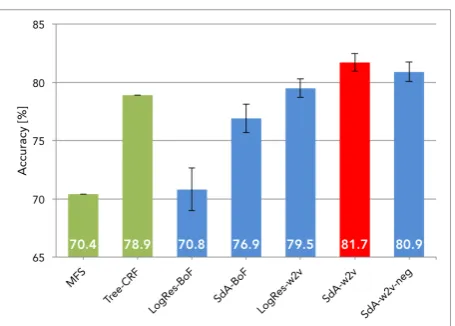
Figure 3: Accuracy of each method with standard error.
4.2 Corpus and tools
We obtained distributed word representations us-ing word2vec4 with Skip-gram (Mikolov et al., 2013b; Mikolov et al., 2013a). We used Japanese Wikipedia’s dump data (2014.11) to learn the 200 dimension distributed representation with word2vec after word-segmentation with MeCab5. The vocab-ulary of the models contains 426,782 words (without processing negation) and 431,782 words (with pro-cessing negation).
The corpus used in the experiment was the Japanese section of NTCIR-6 OPINION (Seki et al., 2007). The data used in our research were the sen-tences from The Mainichi Newspaper and The Japan News articles with polarities annotated by three an-notators. For each sentence, we took the union of the annotations of the three annotators. When the anno-tations were split to both positive and negative, we always used the annotation of the specific annotator. The resulting corpus contained 2,599 sentences. The positive instances comprised 765 sentences whereas the negative instances comprised 1,830 sentences. Although a neutral polarity existed, we ignored it because our task is binary classification.
We performed 10-fold cross validation with 10 threads of parallel processing and evaluated the per-formance of binary classification with accuracy.
4.3 Results
First, Figure 3 shows the accuracy and standard er-rors of each method for the NTCIR-6 corpus.
It can be clearly seen that our method is superior
4
https://code.google.com/p/word2vec/
5
MeCab version-0.996 IPADic version-2.7.0
Table 1: Accuracies of SdA models with different hyper-parameters.
Parameters Accuracy
Noise rate
0% 81.1% 10% 81.5% 20% 81.4% 30% 80.9% 40% 81.1%
50% 81.6%
Number of hidden layers
1 80.6% 2 80.4% 3 81.1%
4 81.6%
5 81.4% 6 81.1%
Number of hidden nodes
100 81.1% 300 81.2%
500 81.3%
700 81.2%
to all baselines, including the state-of-the-art Nak-agawa et al. (2010)’s method by up to 11.3 points. This result shows that the distributed word repretation is sufficiently effective on the Japanese sen-timent classification task, even though only a sim-ple word embedding model, not a comsim-plex tuned representation learning model such as dos Santos et al. (2014)’s, is used.
Note that the parameters of the SdAs above are the best combination of noise rate, number of hid-den layers, and number of hidhid-den nodes (noise rate: 10%, four layers, and 500 dimensions).6
Table 1 contrasts the various hyperparameters. We changed one parameter at a time, while leaving all other parameters fixed. The upper row compares the accuracy of the system with changing noise rate. The best result was obtained when the noise rate was set to 50%. Compared with the standard stacked auto-encoder (noise rate: 0%, accuracy: 81.1%), an SdA with a noise rate of 50% exhibits better accu-racy (81.6%). In the middle of the table, we changed the number of hidden layers. It turned out that, the classifier worked best with four layers. As can be seen, the stacked auto-encoder is superior to the un-stacked one by 1.0 accuracy point. At the bottom of the table, we changed the dimension of hidden nodes. We changed hidden nodes in intervals of 200 dimensions, but the accuracy only fluctuated by
±0.1point. The accuracy was highest when the di-mension was 500.
6
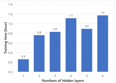
Figure 4: Learning time with varying numbers of hid-den layers.
Figure 5: Learning time with varying dimensions of hidden nodes.
5 Discussion
In this section, we discuss the results of the models (Figure 3), parameter tuning (Table 1), and examples (Table 2).
5.1 Methods
BoF vs. Distributed word representation. When the model was fixed to a linear classifier (lo-gistic regression), the accuracies with Bag-of-Features and distributed word representa-tion were 70.8% and 79.5%, respectively. In contrast, using an SdA, the result for Bag-of-Features was 76.9% and that of distributed word representation was 81.7%. Considering these outcomes, it can be seen that a 4.8 to 8.7 point increase in accuracy occurred when dis-tributed word representation was used. Hence, the contribution of distributed word representa-tion is the largest among the different experi-mental settings.
Linear classifier vs. SdA. The accuracies of lo-gistic regression and SdAs with the same
word vectors made from Bag-of-Features were 70.8% and 76.9%, respectively. With dis-tributed word representation, the accuracy of the linear classifier was 79.6% and that of SdA was 81.7%. Thus, a 2.2 to 6.1 point improve-ment was obtained using SdAs over a tradi-tional linear classifier.
Negation handling. As can be seen in Figure 3, the accuracy of SdA-w2v-neg decreased by 0.8 point compared with SdA-w2v. This differs from Nakagawa et al. (2010)’s report. The reason for this phenomenon may be the data sparseness problem caused by the negation pro-cess. We checked the number of negations in the corpus and found that the numbers of types and tokens are 326 (3.8%) and 1,239 (1.0%), respectively. Thus, the negation process may have little influence on the accuracy.
5.2 Parameters
Figures 4 and 5 show the total training time obtained with 10 parallel processes by changing the numbers of hidden layers and hidden nodes.
Figure 4 shows that the training time grew grad-ually as the number of hidden layers increased. In contrast, Figure 5 shows that the training time dou-bled when the number of hidden nodes was in-creased by 200. These results originate from the structure of SdAs. The nodes of the two adjacent hidden layers are fully connected. Hence, if the network hasl layers and ndimensional nodes, the number of connections will be l ×n×n = ln2. That indicates the relationship between the number of layers and connections is linear, but the number of connections grows exponentially with the num-ber of nodes. Consequently, a small increase in the number of nodes results in a long training time. In contrast, as can be seen from Table 1, the number of nodes has little or no effect on accuracy, whereas changing the number of layers helps to improve the performance.
5.3 Examples
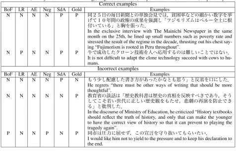
Several examples are presented in Table 2. The val-ues P and N represent the prediction of positive and negative, respectively.
Table 2: Correct and incorrect examples. BoF, LR, AE, Neg, SdA and Gold represent Bag-of-Features, LogRes, Auto-Encoder (one layer SdA without stacking), Negation Processed, Proposal and the Gold answer, respectively.
Correct examples
BoF LR AE Neg SdA Gold Examples
N N N N P P
In the exclusive interview with The Mainichi Newspaper in the same month on the 25th, he lined up small numbers such as poverty rate and stressed the result of the regime in the decade, thrusting out his chest say-ing “Fujimorism is rooted in Peru throughout”.
N P N N P P
It is not difficult to adapt the clone technology succeed with cows to hu-mans.
Incorrect examples
BoF LR AE Neg SdA Gold Examples
N N N N P N
He regrets “there must be other ways of writing that should be more thoughtful”.
N N N N N P
In the discourse of Ministry of Education, he criticized “History textbooks should reflect the truth of history, and only that can make the younger to have the correct view of history so that it can prevent to playing the tragedy again”.
P N N P N P
I would like him not to yield to the pressure and to keep his declaration to the end.
against the data sparseness problem, such as with the coined word “ (Fujimorism)” with which the BoF model is weak. Further, linear clas-sifiers and the unstacked AE fail to handle double negative sentences such as at the bottom. Regard-less of the difficulties, our model copes well with the situation.
Moving on to the wrong answers, it can be seen that our proposed model made human-like mistakes. For example, it mistook the top one containing the word “ (thinking over, reflection, regret),” but it is an ambiguous sentence that might be labeled as positive. Similarly, it failed to classify the middle sentence containing the phrase “
(prevent to replay the tragedy),” which ends with “ (criticize).” The annotations of the above two examples were divided into both positive and negative7. At the bottom, the proposed method did not successfully identify the polarity flipping with the phrase “ (not yield to the pres-sure).” Because the model with negation handling
7
As explained in Section 4.2, we arbitrarily determined the polarity of a sentence when the annotations were split.
answered it correctly, there remains much room for improvement on how to deal with interactions be-tween syntax and semantics (Tai et al., 2015; Socher et al., 2013).
6 Conclusion
In this study, we presented a high performance Japanese sentiment classification method that uses distributed word representation learned from a large-scale corpus with word2vec and a stacked denois-ing auto-encoder. The proposed method requires no dictionaries, complex models, or the engineering of numerous features. Consequently, it can easily be adapted to other tasks and domains without the need for advanced knowledge from experts. In addition, due to the nature of learning with vectors, our sys-tem does not depend on languages.
tree-structured long short-term memory networks. In
Proceedings of the 53rd Annual Meeting of the Associ-ation for ComputAssoci-ational Linguistics and the 7th Inter-national Joint Conference on Natural Language Pro-cessing, pages 1556–1566.
Duyu Tang, Furu Wei, Nan Yang, Ming Zhou, Ting Liu, and Bing Qin. 2014. Learning sentiment-specific word embedding for twitter sentiment classification. In Proceedings of the 52nd Annual Meeting of the Association for Computational Linguistics, volume 1, pages 1555–1565.
Pascal Vincent, Hugo Larochelle, Yoshua Bengio, and Pierre-Antoine Manzagol. 2008. Extracting and com-posing robust features with denoising autoencoders. In
Proceedings of the 25th International Conference on Machine Learning, pages 1096–1103.
Pascal Vincent, Hugo Larochelle, Isabelle Lajoie, Yoshua Bengio, and Pierre-Antoine Manzagol. 2010. Stacked denoising autoencoders: Learning useful representa-tions in a deep network with a local denoising cri-terion. The Journal of Machine Learning Research, 11:3371–3408.
Sida Wang and Christopher D. Manning. 2012. Base-lines and bigrams: Simple, good sentiment and topic classification. In Proceedings of the 50th Annual Meeting of the Association for Computational Linguis-tics, pages 90–94.