ABSTRACT
RIQUELME WON, JUAN ANDRES. Three Essays in Econometric Methods. (Under the direction of Mehmet Caner.)
In this document I present three essays that comprise my doctoral dissertation. These essays
are positioned in the area of inference with instrumental variables setups and model and moment
selection. In the first essay the problem of empirical inference in instrumental variables (iv)
setups where the instruments do that do not perfectly satisfy the exclusion restriction is studied.
The fractionally resampled Anderson–Rubin Berkowitz et al (2012) [Journal of Econometrics,
Vol. 166, pp. 255–266 (2012)] is applied under different scenarios of correlation between the
instruments and the structural variables and used to find empirical bounds to the subsampling
blocks that allows to perform valid inference over the structural parameters. In the second paper
the relative performance of several moment selection criteria currently used in the literature
is compared in terms of (1) how accurate is the moment selection and (2) how good is the
post–estimation performance in term of bias and root mean square errors. The analysis is
performed under different correlation structures in the presence of fixed and diverging number
of moments. In the third paper an alternative estimator to the one in Lee et al (2014) [Journal
of the Royal Statistical Society: Series B, forthcoming] is proposed. This estimator can find the
variables that switch the regimes consistently in a linear setup. The paper starts by showing
that the `∞ bound can be represented as a multiple of the lasso tuning parameter and then this bound is used in a thresholded lasso-type estimator. This estimator achieves a better
Three Essays in Econometric Methods
by
Juan Andres Riquelme Won
A dissertation submitted to the Graduate Faculty of North Carolina State University
in partial fulfillment of the requirements for the Degree of
Doctor of Philosophy
Economics
Raleigh, North Carolina
2015
APPROVED BY:
Barry Goodwin Robert Hammond
Roger von Haefen Mehmet Caner
DEDICATION
BIOGRAPHY
Juan Andres Riquelme Wonwas born in Chile in 1979. He studied at the University of Concepci´on, where he earned a Bachelor Degree in Commercial Engineering with specialization
in Economics, and a Master of Science in Natural Resources and Environmental Economics.
After working for four years as teacher and researcher he started his doctoral studies at North
Carolina State University, USA, and earned his Ph.D in Economics in 2015, specializing in
ACKNOWLEDGEMENTS
I am deeply grateful to my advisor Dr. Mehmet Caner for his constant support, guidance
and encouragement. I also acknowledge the financial support provided by conicyt(Chilean
TABLE OF CONTENTS
LIST OF TABLES . . . vii
LIST OF FIGURES . . . ix
CHAPTER 1 VALID TEST WHEN INSTRUMENTAL VARIABLES DO NOT PER-FECTLY SATISFY THE EXCLUSION RESTRICTION . . . 1
1.1 Preliminaries . . . 1
1.2 Introduction . . . 4
1.3 Inferences When Instruments are not Perfectly Exogenous . . . 5
1.4 The Fractionally Resampled artest . . . 8
1.5 The farcommand . . . 10
1.5.1 Syntax . . . 10
1.5.2 Description . . . 10
1.5.3 Options . . . 10
1.5.4 Saved Results . . . 11
1.5.5 Example . . . 11
1.6 Simulations . . . 21
1.7 Conclusion . . . 24
1.8 References . . . 28
CHAPTER 2 MOMENT AND IV SELECTION APPROACHES: A COMPARATIVE SIMULATION STUDY . . . 35
2.1 Preliminaries . . . 35
2.2 Introduction . . . 36
2.3 Theoretical Framework . . . 39
2.3.1 Moment Selection Methods . . . 39
2.3.2 Parameter Estimation . . . 43
2.4 Monte Carlo Simulations . . . 44
2.5 Results . . . 46
2.5.1 Model Selection . . . 50
2.5.2 Post Selection Performance . . . 51
2.6 Conclusion . . . 54
2.7 Additional Table . . . 59
2.8 References . . . 60
CHAPTER 3 THRESHOLDED LASSO: VARIABLE SELECTION IN HIGH DIMEN-SIONS . . . 62
3.1 Introduction . . . 62
3.2 Weighted Lasso for Threshold Regression . . . 63
3.3 Performance Bounds . . . 65
3.4 Thresholded Weighted Lasso . . . 70
3.4.1 Assumptions in Theorem 3 of Lee et al. (2014) . . . 71
3.5 Monte Carlo Simulations . . . 73
3.6 Conclusion . . . 78
APPENDICES . . . 85
Appendix A A Note on the Use of lars andglmnet . . . 86
A.1 Introduction . . . 86
A.2 The lasso problem . . . 86
A.3 Customizing the λgrid for speed improvement . . . 95
A.4 Conclusion . . . 103
A.5 References . . . 104
Appendix B Compact Storage for High–dimensional Models . . . 105
B.1 Introduction . . . 105
B.2 The key–lock method . . . 105
B.3 Conclusion . . . 111
B.4 References . . . 113
LIST OF TABLES
Table 1.1: Results Saved by thefarcommand . . . 12
Table 1.2: Fractionally resampled Anderson and Rubin test. Default Options. . . 13
Table 1.3: fartest after using the reps()and kappa()options. . . 14
Table 1.4: fartest. Use of the theta() option. . . 14
Table 1.5: fartest. Use of the ci andgrid()options. . . 16
Table 1.6: Ther(ci) matrix. . . 17
Table 1.7: fartest. Use of the kappa() andreps()options. . . 18
Table 1.8: fartest. Use of the ci andgrid()options. . . 18
Table 1.9: Ther(ci) matrix. . . 19
Table 1.10: Size of thefar test at θ0= 0. . . 23
Table 1.11: Power of thefartest at θ0= 0, covariance setup 1. . . 25
Table 1.12: Power of thefartest at θ0= 0, covariance setup 2. . . 26
Table 1.13: Power of thefartest at θ0= 0, covariance setup 3. . . 27
Table 2.1: Summary of the Performance of the Moment Selection Techniques . . . 48
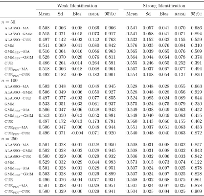
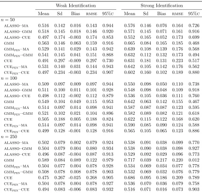
Table 2.2: Summary of the Performance of the Post Selection Techniques . . . 49
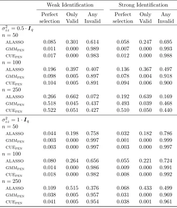
Table 2.3: Probabilities: Moment Selection Criteria. Setup 1 . . . 52
Table 2.4: Probabilities: Moment Selection Criteria. Setup 2 . . . 53
Table 2.5: Monte Carlo results for ˆθ. Setup 1,σzz2 = 0.5·Iq. . . 55
Table 2.6: Monte Carlo results for ˆθ. Setup 1,σzz2 = 1·Iq. . . 56
Table 2.7: Monte Carlo results for ˆθ. Setup 2,σ2zz = 0.5·Iq. . . 57
Table 2.8: Monte Carlo results for ˆθ. Setup 2,σzz2 = 1·Iq. . . 58
Table 2.9: R2 of the First Stage Estimation for Each Method . . . 59
Table 3.1: Simulation Results forM = 50, ρ= 0,n= 200 . . . 80
Table 3.2: Lasso and Thresholded Lasso,ρ= 0, Increasing Number of Observations . 81 Table 3.3: Lasso and Thresholded Lasso,ρ= 0, Increasing Number of Variables . . . 82
Table 3.4: Lasso and Thresholded Lasso,ρ= 0,D =Ip . . . 83
Table 3.5: Lasso and Thresholded Lasso,ρ= 0,q =X(1). . . 84
Table A.1: Parameters estimates. . . 89
Table A.2: Results forλ= 10. . . 90
Table A.3: Results after scaling. . . 92
Table A.4: Results after scaling using theexactoption. . . 93
Table A.5: Results for fixed lambda. . . 94
Table A.6: Scaling factors forλfor some common lasso problems . . . 95
Table A.7: Results with the modified grid. . . 97
Table A.8: Results from using the custom grid. . . 99
Table A.9: Comparison of the three proposed approaches. . . 101
Table B.1: Output from thebincomb() function. . . 107
Table C.1: Simulation Results forM = 50, ρ= 0.3,n= 200 . . . 115
Table C.2: Lasso and Thresholded Lasso,ρ= 0.3, Increasing Number of Observations 116 Table C.3: Lasso and Thresholded Lasso,ρ= 0.3, Increasing Number of Variables . . 117
LIST OF FIGURES
Figure 1.1: Code line using thefarcommand syntax. . . 13
Figure 1.2: Code to use thereps()and kappa() options. . . 14
Figure 1.3: Code to use thetheta() option. . . 14
Figure 1.4: Code to use theci() option. . . 15
Figure 1.5: Code to use thegrid()option. . . 15
Figure 1.6: Code to call ther(ci)matrix. . . 16
Figure 1.7: Code to modify theκ value. . . 17
Figure 1.8: Code to call ther(ci)matrix. . . 18
Figure 1.9: Code to call ther(ci)matrix. . . 19
Figure 1.10: Code to get the upper limit of the 95% confidence interval. . . 20
Figure 1.11: Source code of thefarcommand . . . 30
Figure A.1: Loading of thelars and glmnetpackages. . . 87
Figure A.2: Parameter setup. . . 88
Figure A.3: Data generation. . . 88
Figure A.4: Creation of thelarsand glmnetobjects. . . 88
Figure A.5: Code to get the lasso parameters. . . 89
Figure A.6: Suppression of the Standardization. . . 90
Figure A.7: Code to scale theglmnetestimator. . . 91
Figure A.8: Use of theexactoption. . . 93
Figure A.9: Scaling with fixed lambda. . . 94
Figure A.10:The default grid. . . 96
Figure A.11:Modified grid. . . 96
Figure A.12:Estimation with the modified grid. . . 96
Figure A.13:Modification of theglmnetdefault grid. . . 98
Figure A.14:Custom grid estimation . . . 98
Figure A.15:Themethod1() function. . . 99
Figure A.16:Themethod2() function. . . 100
Figure A.17:Themethod3() function. . . 100
Figure A.18:Code to compare the three proposed approaches. . . 101
Figure A.19:Execution times for each method, 1000 repetitions . . . 102
Figure B.1: Thebincomb() function. . . 106
Figure B.2: Call to thebincomb() fuunction. . . 106
Figure B.3: Size of the combination matrix. . . 107
Figure B.4: Thegencomb() function. . . 108
Figure B.5: List after using thegencomb function. . . 109
Figure B.6: Size of the combinations list. . . 109
Figure B.7: Theindexes function. . . 110
Figure B.8: Output of theindexes function. . . 110
Figure B.9: Another output of theindexes function. . . 110
Figure B.10: Therev.indexesfunction. . . 111
C h a p t e r 1 : Va l i d t e s t s w h e n i n s t r u m e n ta l va r i a b l e s d o n o t
p e r f e c t ly s at i s f y t h e e x c l u s i o n r e s t r i c t i o n
1.1
Preliminaries
This chapter is intended for the applied researcher that is not sure about the validity of their
instruments in an instrumental variables estimation setup. In particular, we consider situations
in which the instruments do not perfectly satisfy the exclusion restriction, but come close to it.
This situation is common in the applied literature when the instrumental variables approach is
used. For example Acemoglu et al. (2001) use early settler mortality data from as far back as
the fifteenth and sixteenth centuries as an instrument for contemporary institutions, Angrist
(1990) use draft lotteries as instrument for the veteran status to study lifetime earnings, and
Card (1995) uses a variable measuring whether a man grew up in the vicinity of a four–year
college as instrument for estimating the returns to schooling. In each case, however, there are
good reasons to believe that the exclusion restriction is not necessarily perfect (for technical
details see Wooldridge (2002), pp. 89–90.)
In this chapter we give a non–technical description of a modification of the Anderson–Rubin
(1949) test proposed by Berkowitz, Caner and Fang (2012) that accounts for violations of the
this test is that in small sample sizes, the resampling blocks can be modified to obtain valid
critical values. We work under the following ivsetup:
y =W B+Y θ0+u
Y =WΓ +ZΠ +V
whereyis an×1 vector of outcomes,nis the sample size,Y is an×mmatrix of endogenous
variables andZ is an×kmatrix of instruments, the magnitude of the block size modification is
data–driven and it is assumed that the violation of the exclusion restriction has a local–to–zero
form:
E[Zjuj] =
C
√
n
where C is a k×1 vector (one component for each instrument), and each element of C,
denoted by Cj (j = 1, . . . , k) is a constant. The sign of each Cj depends on the sign of the
covariance between thej-th instrument and the error term. The proof in Berkowitz, Caner and
Fang (2012) require only that Cj belong to a compact subset ofRk, but their specific values are unknown. This poses a challenge to the empirical researcher since the modification to the
resampling block sizes are depending on the value ofCj and can lead to different results when
testing the exclusion restriction.
This chapter has three main objectives:
1. To implement an estimation tool for the fartest for applied researchers.
2. To analyze the size and power properties of the far test under different covariance
structures and degrees of violation of the exclusion restriction.
3. Make use of these results to find numerical bounds for the vector C.
Using this command, extensive simulations are performed to achieve the objective number two.
These simulations provide the empirical bounds for Cj and the resampling block sizes. Our
results for small samples exhibit good size and power combinations when we select approximately
the 20–25% of the total sample for the resampling block sizes. The use of this percentages is
proposed as a rule of thumb.
The source code is provided in the last section of the chapter and can be installed directly
1.2
Introduction
Instrumental variables methods are used in economics to study major questions including the
impact of institutions on economic performance and the returns to schooling. Valid instruments
must be relevant and exogenous. In the case of relevance, there has been substantial progress
made in understanding the asymptotic properties of weak instruments. Stock and Wright (2000)
show how the Anderson and Rubin (1949) test (for herein, denoted theartest) can be used to
draw valid inferences when the instruments are weak.
In the case of exogeneity, however, there is a growing concern among researchers about the
difficulty of picking instruments that perfectly satisfy the exclusion restriction. For example, in
an influential study of the impact of institutions on long run growth, Acemoglu et al. (2001)
use early settler mortality data from as far back as the fifteenth and sixteenth centuries as an
instrument for contemporary institutions∗. Glaeser, La Porta, Lopez-de-Silanes and Shleifer (2004) argue that the early settlers brought their attitudes about education to their colonies,
affecting the long run growth through their influence on the human capital accumulation process.
In a similar manner, draft lotteries (Angrist, 1990) and whether a man grew up in the vicinity
of a four-year college (Card, 1995) are influential instruments for estimating the returns to
schooling. In each case, however, there are good reasons to believe that the exclusion restriction
is not necessarily perfect (See Wooldridge (2002), pp. 89-90).
This chapter contains a non-technical summary of the new test statistic derived in Berkowitz,
Caner and Fang (2012) for instruments that come “close” to satisfying the exclusion restriction
but do not satisfy it perfectly. In our analysis, we use the ar test because it is robust to
weak identification. However, because the ar test uses the overly strong assumption that
an instrument is perfectly exogenous it can have bad small sample properties (Caner, 2010;
∗
Guggenberger, 2012). The fractionally resampled ar(far) test modifies the artest based on
results from Wu (1990, section 2) accounting for the extent to which an instrument violates the
orthogonality condition and it is not oversized in large samples.
The rest of the chapter is as follows: In Section 1.3 we describe the artest in a setup that
allows for instruments that do not perfectly satisfy the orthogonality condition. Section 1.4
summarizes the far test and shows how the block size for the far test can be adjusted to
improve the test size and power. Section 1.5 describes the syntax and output of our user-written
stataprogram and discusses the different available options using an example from Acemoglu et al. (2001, 2011). Section 1.6 presents the results of size and power simulations under different
levels of violation of the orthogonality condition. Section 1.7 concludes.
1.3
Inferences When Instruments are not Perfectly Exogenous
Consider the following setup:
y=W B+Y θ0+u (1.1)
Y =WΓ +ZΠ +V (1.2)
In this system of equations, y is an×1 vector of outcomes, n is the sample size, Y is a
n×m matrix of endogenous variables andZ is an×k matrix of instruments. For example,y
can be long rungnp per capita, ndenotes the number of countries that are former colonies and
Y is a set of contemporary institutions. In Acemoglu and Johnson (2005)m= 2, and includes
property rights and contract enforcement. For simplicity, and without loss of generality, we
consider the case where Y is a n×1 vector of property rights institutions.
There are a host of exogenous covariates in W, which is a n×l matrix. For example, if
l = 3, then W could include gnp, human capital and temperature in 1960. The coefficients
W from the system. By using the projection matrixP =W(W0W)−1W0 we define:
yW =y−P y
ZW =Z−P Z
YW =Y −P Y
And the system of equations in (1.1) and (1.2) can be written as:
yW =YWθ0+uW (1.3)
YW =ZWΠ +VW (1.4)
thus, the vector W of covariates can be ignored.
In Acemoglu et al. (2001), the parameter of interest θ0 in equation (1.3) is the impact of
institutions on long run growth. Because long rungnpper capita also influences institutions and
there are potentially omitted variables in the residual uW that influence both institutions and gdpper capita, the variable Y is endogenous. Technically this means thatcov(YW, uW)6= 0. In
order to correct for the endogeneity of institutions, an instrument or a set of instruments,ZW is
used as an exogenous source of variation for institutions. The instruments satisfy the condition:
E[ZW iVW i0 ] = 0, i= 1, . . . , n (1.5)
Acemoglu et al. (2001) use early settler mortality data from hundreds of years ago as an
instrument for contemporary institutions.
There is large literature for drawing inferences when instruments are weak but still sufficiently
relevant (Stock and Wright, 2000) and there are now commands for implementing valid tests in
stata(see Moreira and Poi, 2003). Here we consider tests for instruments that are not perfectly exogenous, in which case the standard t-statistic and thear test for testingH0 :θ=θ0 have
as in equation (1.5). More realistically, a set of instruments may exhibit near exogeneity as
follows:
E[ZW iuW i] =
C
√
n (1.6)
Equation (1.6) allows for a slight covariance between the instruments and the error term.
C is a k×1 vector (one component for each instrument), and each element ofC, denoted by
Cj (j = 1, . . . , k) is a constant. The sign of each Cj depends on the sign of the covariance
between thej-th instrument and the error term. For example, when k= 2, then we can have
C= (−1,2)0. For simplicity and without loss of generality we assume that the upper and lower bound of the set containing theCj values are the same for all the instruments. Further technical
details are described in the section 2 of Berkowitz, Caner and Fang (2012).
In order test the null hypothesis H0 :θ =θ0, the ar-test is preferred for several reasons.
First, it can be used when the instruments are weak. Moreover, Guggenberger (2012) shows
that the ar-test is the best choice for limiting size distortion when the exclusion restriction
is slightly violated. Caner (2010) also shows that the ar-test is slightly oversized in a many
instruments framework.
Let then×1 vector of residuals of the structural equation under the null be denoteduW(θ0):
uW(θ0) =yW −YWθ0 (1.7)
Then, the ar test for testingH0:θ=θ0, assumes thatC= 0 (i.e., the instruments perfectly
satisfy the exclusion restriction). The test statistic is given by:
AR(θ0) =n×S¯n0(θ0) ˆΩ−1S¯n(θ0) (1.8)
where ˆΩ = 1nPn
i=1ZW iZ
0
W i(uW(θ0))2 and ¯Sn(θ0) =
hZ0
WuW(θ0) n
i
k×1 vector of estimated covariances between the instruments and the residuals in the structural
equation under the null hypothesisH0 :θ=θ0.
The limiting distribution of the ar test is central chi square with k degrees of freedom.
Berkowitz, Caner and Fang (2008, 2012) show that the ar–test over–rejects the null when the
orthogonality condition is not perfectly satisfied. Moreover, in small samples the test can be
oversized even when the correlation between the instruments and structural error is close to zero.
This size distortion gets worse as the correlation between an instrument and the structural error
terms gets stronger. This problem arises because thear–test assumes that C= 0 in equation
(1.6). In the next section we explain how the fartest accounts forC 6= 0 and, thus, allow the
researcher to draw valid, but conservative inferences.
1.4
The Fractionally Resampled
ar
test
The far test uses Wu’s (1990) jackknife histogram estimator to recover the limits of the
population mean of θ by taking a subset of sizeb from then observations in the full sample.
There are nb
blocks of size b with equal probability of being selected, which are drawn via
simple random sampling without replacement. To test the null hypothesisH0:θ=θ0, we need
to estimateZW0 uW(θ0). Following Berkowitz, Caner and Fang (2012) we use the subscript (*) to label the resampled estimates. Using this notation thefar test can be written as:
F AR(θ0) =
bS¯b0(θ0) ˆΩ−1S¯b(θ0)
(1−f) (1.9)
where ¯Sb(θ0) = Pb
i=1Ziui
b andf is the fraction of the sample that generates the block of size
b.∗ Note that ˆΩ is obtained from the full sample and replaced by (1−f) ˆΩ in each iteration. From Theorem 1 in Berkowitz, Caner and Fang (2012), pp. 258, under suitable assumptions the
statistic Jb(t) =P∗(F AR(θ0)≤t), whereP∗ stands for the resampled probability, converges to ∗
φmf(t), the cumulative distribution of
1 +
√
f
√
1−f
2
χ2k,nc (1.10)
where χ2k,nc is the non-central χ2 with k degrees of freedom and noncentrality parameter nc = 1+2√1
f√1−f CΩ−1C
2 . If half of the sample is resampled, f = 1/2 and the limit in (1.10) becomes:
4χ2k+ 4C0Ω−1L+C0Ω−1C (1.11)
where L≡N(0,1) whereas the artest limit is
χ2k+ 2C0Ω−1L+C0Ω−1C
Equation (1.11) is used for testing H0 : θ = θ0 when C 6= 0 and corrects for the size
distortions obtained in the standard artest. This version of thefar test is very conservative,
especially in small samples. To correct for this, Theorem 1 in Berkowitz, Caner and Fang (2012),
pp. 258, shows that the resampled fractionf can be modified:
fn= 1/2−κn (1.12)
Whereκn>0 is a data driven deterministic sequence converging to 0. In practice,κn=κ/ √
n
is used. For example if n= 100 andκ= 2.5 thenκn= 2.5/ √
100 = 0.25 andfn= 0.25, so each
resampling consists of 25 observations. κn= 2.5/ √
nprovides good power in our simulations,
and κn = 3/ √
n is recommended when the researcher is confident that that the instrument
comes close to perfectly satisfying the exclusion restriction.
Our user-written farcommand takes advantage of the flexibility and fast execution of the
The command is introduced in the next section.
1.5
The
far
command
1.5.1 Syntax
far depvar
varlist 1
(varlist2 = varlist iv)if
in
, reps(#) kappa(#) theta(numlist1) ci
grid(numlist2) level(#)
1.5.2 Description
The farcommand performs the Fractionally Resampled Anderson Rubin test
(Berkowitz, Caner and Fang, 2012) for the joint significance of the endogenous regressors in an
instrumental variables regression ofdepvar using the optional controls invarlist1, the endogenous
regressors invarlist2 and the instrumental variables invarlist iv.
1.5.3 Options
The following options are provided:
reps(#)specifies the number of repetitions of the resampling procedure. A large number of repetitions is necessary for the results in the section 1.4 to be valid. The default value is
reps(10000) and it gives fast and reliable estimates in small samples (n < 100). If the number of repetitions is not large enough, the fartest p-values may vary.
kappa(#)specifies the value of the κ constant. Note thatκn=κ/ √
nin equation (1.12). Any
positive real number can be used. The default value is kappa(3)(see the simulations section for the justification of the selected default value).
is not specified the farcommand will perform a significance test (all the values in numlist1 will be set as zero). By implementing this option the far test can be inverted to find
confidence intervals for θ0.
cienables the user to test for a grid of different values ofθ0 and search for the (1−α)% confidence interval for the true scalarθ. The significance level and the grid can be customized by using
the options level(#)andgrid(numlist2). This option is available when there is only one endogenous variable.
level(#)is the significance level for the test in the grid search. The default value islevel(95).
grid(numlist2)specifies the grid for the values ofθ0 to be tested. numlist2 consists of three elements: the minimum level, the maximum level and the increments of the grid. The default
values aregrid(-30, 30, 0.01).
1.5.4 Saved Results
As an r-class command, farstores the results in the Table 1.1: We use an example to illustrate the use of the farcommand.
1.5.5 Example
Acemoglu, Johnson and Robinson (2001) use two stage least squares methods to estimate
the effect of institutions on long run economic growth. Their baseline data set consists of 64
countries that are former European colonies. They use the log of per-capita gdp using ppp
(purchasing power corrected) prices (logpgp95) as the measure of long run growth, an index of
protection against expropriation during 1985-95 (avexpr) as the measure of institutions and
the log early settler mortality of colonizers (logem4) as the instrument for institutions. The
fundamental identifying assumption then is that early settler mortality influences long term
growth exclusively through the quality of contemporary institutions (see equation (1.5)).
Table 1.1: Results Saved by the farcommand
Scalars
r(ar) Full samplearStatistic r(arp) Full samplep-value
r(farp) arp-value r(reps) Resampling repetitions
r(kappa) The constantκ r(k) Number of instruments
r(l) Number of controls r(m) Number of endogenous
r(n) Number of observations variables
Macros
r(title) Title in the output r(cmdline) Executed command line
r(depvar) Dependent variable r(exogenous) List of controls
r(endogenous) List of endogenous r(instruments) List of instruments
variables r(grid) Grid values
Matrices
r(theta) Endogenous parameters tested
r(ci) Fractionally resampled p-values for the parame-ters in the grid
robustness checks is the incidence of malaria in 1994 (malfal94). There are two missing
values for this variable, which reduces the sample size to 62. This control is critical for their
exclusion restriction because it offsets the potential impact of early settler mortality through
the contemporary disease environment. However, even after controlling for the contemporary
disease environment, there are still reasons to argue that the exclusion restriction that Acemoglu,
Johnson and Robinson (2001) employ is not perfect (see, for example, Glaeser et al. 2004). Thus,
we relax the strict exclusion restriction in equation (1.5) and allow for the early settler mortality
instrument to exhibit near exogeneity as in equation (1.6). We compare the arandfartest to
examine how the potential correlation between the instrument and structural error will affect
inference∗. In the next 2 command lines we load the local data filefardata.dtaand call the ∗
Acemoglu et al. (2011) point out that the inclusion of the variablemalfal94 is “highly problematic” because the current prevalence of malaria is endogenous. In our example we includemalfal94 to show how ourfar
farcommand for the specified iv regression∗:
. use fardata, clear
. far logpgp95 malfal94 (avexp = logem4)
Figure 1.1: Code line using thefarcommand syntax.
Table 1.2: Fractionally resampled Anderson and Rubin test. Default Options.
Full sample Full sample FAR
statistic p-value p-value reps N
AR-Test 5.5421 0.0186 0.1462 10000 62
The output in the Table 1.2 displays the full sample ar statistic, the full sample and
the fractionally resampled p-values, the number of resampling repetitions and the number of
observations. In this case under the full samplear test, the hypothesis H0 :θ0= 0 is rejected
at 5% (with ap-value of 1.86%), but thefar test does not reject it. This is consistent with the
result in equation 1.11 that shows that thefar is a more conservative test.
To show other available options of thefar command we perform the same hypothesis test, but this time we increased the number of repetitions to 100,000 and set κ= 2. Note that the
null is not rejected at the 15% under thefar test after decreasing κ (see Table 1.3):
∗
. far logpgp95 malfal94 (avexp = logem4), reps(100000) kappa(2)
Figure 1.2: Code to use the reps()andkappa() options.
Table 1.3: far test after using the reps()andkappa() options.
Full sample Full sample FAR
statistic p-value p-value reps N
AR-Test 5.5421 0.0186 0.1505 100000 62
To test if the θ0 parameter is equal to (say) 3, use:
. far logpgp95 malfal94 (avexp = logem4), theta(3)
Figure 1.3: Code to use the theta() option.
Table 1.4: fartest. Use of the theta()option.
Full sample Full sample FAR
statistic p-value p-value reps N
Note that the p-value of the far test increases when testingH0 :θ0= 3. We have rejected
that θ0 is equal to 0 and 3 already. To look for theθ0 values for which the null hypothesis is not
rejected at some fixed α significance level we can perform a grid search. The implementation of
the grid search is done by using theci option. To test the null under the default grid∗ simply use
. far logpgp malfal94 (avexp = logem4), ci
(output omitted)
Figure 1.4: Code to use the ci() option.
We are not presenting the default grid here due to its extension.† The user can list the grid stored in ther(ci)matrix to inspect it. It is enough to say that all thefarp-values are greater than 0.05, thus the 95% confidence interval forθ0 obtained from this search is [−∞,+∞]. A
portion of the default grid can be displayed using the lines in the Figures 1.5 and 1.6.
. far logpgp95 malfal94 (avexp = logem4), ci grid(-1,1,0.1)
Figure 1.5: Code to use thegrid()option.
∗
This is equivalent to execute:
. far logpgp malfal94 (avexp = logem4), ci grid(-30, 30, 0.01) level(95) †
Table 1.5: far test. Use of the ciand grid()options.
Full sample Full sample FAR
statistic p-value p-value reps N
AR-Test 5.5421 0.0186 0.1495 10000 62
. matrix list r(ci)
Figure 1.6: Code to call ther(ci) matrix.
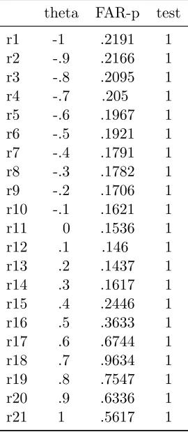
The first column of the r(ci)matrix in the Table 1.6 contains the grid ofθ0 values defined by the grid(numlist2)option. The second column corresponds to thefartest p-values at each differentθ0 values. The third column contains a dummy variable that takes the value of 1 if the
corresponding θ0 is included in the confidence interval defined by theleveloption (this occurs if thep-value in the column 2 is greater than the critical α level).
The default confidence level corresponds to anα level of 5%, therefore the elements in the
third column will be one if the corresponding far p-value is greater than 0.05. In the next
example we derive a bounded confidence interval. In the light of the debate between Albouy
(2008) and Acemoglu, Johnson and Robinson (2001), Acemoglu, Johnson and Robinson (2011)
recommend capping the settler mortality at 250 per 1,000 per annum. We can generate a
transformed variable, estimate thearandfartest and perform the grid search in two command
lines. We increased the number of resampling repetitions to 100,000 to improve the precision of
the estimated interval and setκ= 3.1 to show the full usage of the grid search:
Table 1.6: Ther(ci) matrix.
theta FAR-p test
r1 -1 .2191 1
r2 -.9 .2166 1
r3 -.8 .2095 1
r4 -.7 .205 1
r5 -.6 .1967 1
r6 -.5 .1921 1
r7 -.4 .1791 1
r8 -.3 .1782 1
r9 -.2 .1706 1
r10 -.1 .1621 1
r11 0 .1536 1
r12 .1 .146 1
r13 .2 .1437 1
r14 .3 .1617 1
r15 .4 .2446 1
r16 .5 .3633 1
r17 .6 .6744 1
r18 .7 .9634 1
r19 .8 .7547 1
r20 .9 .6336 1
r21 1 .5617 1
. gen malaria250 = min(malfal94, 0.250) if malfal != . (2 missing values generated)
. far logpgp95 malaria250 (avexp = logem4), kappa(3.1) reps(100000)
Table 1.7: far test. Use of thekappa() and reps()options.
Full sample Full sample FAR
statistic p-value p-value reps N
AR-Test 9.2185 0.0024 0.0180 100000 62
search gives a 95% confidence interval forθ0 of [0.34; 4.39]. Acemoglu et al. (2011) obtained the
confidence interval [0.27; 0.95] using the ar test and including other covariates. Ours is more
conservative, but it does not suffer the small sample problems discussed in Section 1.3.
The lower limit of the confidence interval can be obtained using the following command line:
. far logpgp95 malaria250 (avexp = logem4), kappa(3.1) reps(10000) ci > grid(.3,.5,.01)
Figure 1.8: Code to call ther(ci) matrix.
Table 1.8: far test. Use of the ciand grid()options.
Full sample Full sample FAR
statistic p-value p-value reps N
. matrix list r(ci)
Figure 1.9: Code to call ther(ci) matrix.
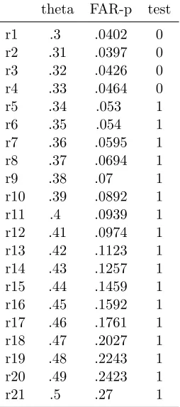
Table 1.9: Ther(ci) matrix.
theta FAR-p test
r1 .3 .0402 0 r2 .31 .0397 0 r3 .32 .0426 0 r4 .33 .0464 0 r5 .34 .053 1 r6 .35 .054 1 r7 .36 .0595 1 r8 .37 .0694 1 r9 .38 .07 1 r10 .39 .0892 1 r11 .4 .0939 1 r12 .41 .0974 1 r13 .42 .1123 1 r14 .43 .1257 1 r15 .44 .1459 1 r16 .45 .1592 1 r17 .46 .1761 1 r18 .47 .2027 1 r19 .48 .2243 1 r20 .49 .2423 1 r21 .5 .27 1
By inspecting the grid in the Table 1.9, it is easy to see that the lower limit of the interval is
To make the dummy in the third column take the value 1 based on the two decimal places
roundedfarp-values, the user must set the confidence level to 95.5. In this example the rounded
lower limit is 0.33.
In a similar manner, the upper limit can be obtained by using:
. far logpgp malaria250 (avexp=logem4), reps(100000) ci kappa(3.1) > grid(4.3,4.5,0.01)
Figure 1.10: Code to get the upper limit of the 95% confidence interval.
This last result is for illustrative purposes and it needs to be carefully considered. With
a sample of 62 observations, selecting κ = 3.1 corresponds to a resampled fraction f = 0.11,
which implies a block size of size b= 7. This fraction is too small. As the block size diminishes,
the resampling technique turns into a subsampling procedure and Berkowitz, Caner and Fang
(2012) (section 4) show that as f → 0 the ar test is always oversized. We choose κ = 3.1
only because it generates a bounded interval although in our simulations we find that the best
combinations of size and power are obtained by selecting sub-sample sizes between 20–25%
of the total observations. κ values that generates f <0.2 generates unreliable and unstable
results but there should be further examination of this topic. In our example the best choice is
κ <2. The statistical implications of the estimates obtained by this smallerκ values and the
best choice of the block size are beyond the scope of this chapter.
In order to empirically obtain valid confidence intervals we suggest exploring the default
grid under κ values that corresponds to f above 0.2 to check the overall sequence of the test
trials to find the presented bounded interval for this data set. In general the confidence set can
be bounded, disjoint or even infinite if the model is misspecified, which implies that the grid
search might become excessively time consuming. We believe that the option of user-defined
grids gives the researcher enough flexibility for finding a solution that is not too time consuming
and not too computationally intensive.
1.6
Simulations
To choose the default value of the constantκ in the farcommand we simulated the system of equations in (1.3) and (1.4) under different scenarios in which the exclusion condition is violated
and explore the far test size and power properties. We choose scenarios similar to those in
Berkowitz, Caner and Fang (2012), but with smaller correlations between the structural error
and the instruments. For empirical purposes we assume that the researcher chooses imperfect
instruments that come close to satisfying the exclusion restriction, so the covariance between
the instruments and the residuals in the structural equation is very small, but nonzero. The
data forzi, ui, vi is generated from a joint normal distribution N(0,Σ) where:
Σ =
1 σzu 0
σzu 1 0.9
0 0.9 1
(1.13)
were σzu=cov(ZW iuW i).
In equation (1.13) we setup σz2 = σ2u = σv2 = 1, σzv = 0 and σuv = 0.9. Note that the
upper-left 2×2 submatrix corresponds to our simulated version of the Ω matrix in equation
In the first setup we have σzu local to zero as in equation (1.6):
σzu =
h
√
n
and we choose h equal to 0.5 and 1 for the simulations. The largerh becomes, the worse is
the selected instrument.
The second setup corresponds toσzu constant:
σzu=D
and we chose Dequal to 0.1 and 0.25 for the simulations.
In the third setup we have σzu consistent with the bounds of the compact set containing C:
σzu=
an1/3 n1/2
and ais equal to 0.25 and 0.5 in the simulations.
To explore the size properties of the fartest we simulate one endogenous variable (m= 1),
one instrument (k = 1) and two controls (l= 2), one of them being a constant: B = (1,2)0. To model strong identification we set Π = 2 in equation (1.4). We get the similar results (not
reported) for the weak identification case. The sample size nis equal to 100 and 200 and κ is
equal to 1.5, 2, 2.5 and 3, so κn is equal to 1.5/ √
n, 2/√n, 2.5/√nand 3/√n in the equation
(1.12). We give the data a heteroskedastic structure by using the following error form:
u∗W i= abs(ZW i)uW i
Each scenario was simulated 1,000 times using 1,000 resampling iterations. The results for
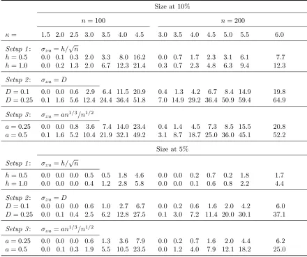
patterns than those found by Berkowitz, Caner and Fang (2012). Given that our correlations
are smaller, the test is undersized whenκn is equal 1.5/ √
nand 2/√n, but but the undersize is
corrected when κn is equal 2.5/ √
n and 3/√n, especially in setups 2 and 3 when the sample
size is 100. Note that when n = 200 the far test is undersized in all the setups due to its
conservative nature.
Table 1.10: Size of thefar test at θ0= 0.
Size at 10%
n= 100 n= 200
κ= 1.5 2.0 2.5 3.0 3.5 4.0 4.5 3.0 3.5 4.0 4.5 5.0 5.5 6.0
Setup 1: σzu=h/
√
n
h= 0.5 0.0 0.1 0.3 2.0 3.3 8.0 16.2 0.0 0.7 1.7 2.3 3.1 6.1 7.7
h= 1.0 0.0 0.2 1.3 2.0 6.7 12.3 21.4 0.3 0.7 2.3 4.8 6.3 9.4 12.3
Setup 2: σzu=D
D= 0.1 0.0 0.0 0.6 2.9 6.4 11.5 20.9 0.4 1.3 4.2 6.7 8.4 14.9 19.8
D= 0.25 0.1 1.6 5.6 12.4 24.4 36.4 51.8 7.0 14.9 29.2 36.4 50.9 59.4 64.9
Setup 3: σzu=an1/3/n1/2
a= 0.25 0.0 0.0 0.8 3.6 7.4 14.0 23.4 0.4 1.4 4.5 7.3 8.5 15.5 20.8
a= 0.5 0.1 1.6 5.2 10.4 21.9 32.1 49.2 3.1 8.7 18.7 25.0 36.0 45.1 52.2
Size at 5%
Setup 1: σzu=h/
√
n
h= 0.5 0.0 0.0 0.0 0.5 0.5 1.8 4.6 0.0 0.0 0.2 0.7 0.2 1.8 1.7
h= 1.0 0.0 0.0 0.0 0.4 1.2 2.8 5.8 0.0 0.0 0.1 0.6 0.8 2.2 4.4
Setup 2: σzu=D
D= 0.1 0.0 0.0 0.0 0.6 1.0 2.7 6.7 0.0 0.2 0.6 1.6 2.0 4.2 6.0
D= 0.25 0.0 0.1 0.4 2.5 6.2 12.8 27.5 0.1 3.0 7.2 11.4 20.0 30.1 37.1
Setup 3: σzu=an1/3/n1/2
a= 0.25 0.0 0.0 0.0 0.6 1.3 3.6 7.9 0.0 0.2 0.7 1.6 2.0 4.4 6.2
a= 0.5 0.0 0.1 0.3 1.9 5.5 10.5 23.5 0.0 1.2 4.0 7.9 12.1 18.2 25.0
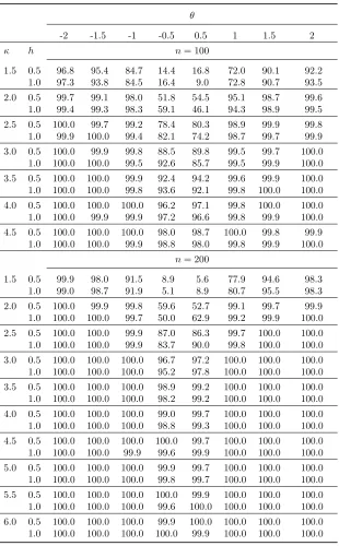
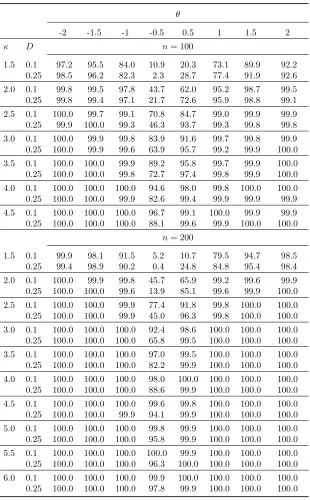
To explore the power properties of the fartest, we simulate scenarios with θ0 equal to −2,
−1.5,−1,−0.5, 0.5, 1, 1.5 and 2 and tested for θ0 = 0. The results are presented in the Tables
1.11, 1.12 and 1.13. We focus on power and not in size-adjusted power because the fartest uses
only one critical value in its application. The simulation exercise shows the test has low power
when θ0 is equal to -0.5 and 0.5 and κn is equal to 1.5/ √
nand 2/√n. The power improves
whenκnis equal to 2.5/ √
nand 3/√n. Considering these results we decided to setκ= 3 as the
default value in the farcommand. Thisκ value is the one that gave us the best size and power combinations and corresponds to a resampling fractionf = 0.2 whenn= 100. The researcher
can easily adjust κ to obtain resampling fractions above the 20% of the total sample. Lowerf
values generates unreliable and unstable results as discussed in section 1.5. Further discussion
and other setups for the covariance matrix can be found in Berkowitz, Caner and Fang (2012).
1.7
Conclusion
We have shown how the fartest can be used to draw valid inferences when the instruments
do not perfectly satisfy the exclusion condition. Our simulations for n = 100 exhibit good
size and power combinations when we select approximately the 20–25% of the total sample
for the resampling block sizes. This corresponds to κn = 3/ √
n in equation (1.6). κ values
that generate smaller block sizes are not recommended. By taking advantage of the speed of
Table 1.11: Power of thefar test at θ0= 0, covariance setup 1.
θ
-2 -1.5 -1 -0.5 0.5 1 1.5 2
κ h n= 100
1.5 0.5 96.8 95.4 84.7 14.4 16.8 72.0 90.1 92.2
1.0 97.3 93.8 84.5 16.4 9.0 72.8 90.7 93.5
2.0 0.5 99.7 99.1 98.0 51.8 54.5 95.1 98.7 99.6
1.0 99.4 99.3 98.3 59.1 46.1 94.3 98.9 99.5
2.5 0.5 100.0 99.7 99.2 78.4 80.3 98.9 99.9 99.8
1.0 99.9 100.0 99.4 82.1 74.2 98.7 99.7 99.9
3.0 0.5 100.0 99.9 99.8 88.5 89.8 99.5 99.7 100.0
1.0 100.0 100.0 99.5 92.6 85.7 99.5 99.9 100.0
3.5 0.5 100.0 100.0 99.9 92.4 94.2 99.6 99.9 100.0
1.0 100.0 100.0 99.8 93.6 92.1 99.8 100.0 100.0
4.0 0.5 100.0 100.0 100.0 96.2 97.1 99.8 100.0 100.0
1.0 100.0 99.9 99.9 97.2 96.6 99.8 99.9 100.0
4.5 0.5 100.0 100.0 100.0 98.0 98.7 100.0 99.8 99.9
1.0 100.0 100.0 99.9 98.8 98.0 99.8 99.9 100.0
n= 200
1.5 0.5 99.9 98.0 91.5 8.9 5.6 77.9 94.6 98.3
1.0 99.0 98.7 91.9 5.1 8.9 80.7 95.5 98.3
2.0 0.5 100.0 99.9 99.8 59.6 52.7 99.1 99.7 99.9
1.0 100.0 100.0 99.7 50.0 62.9 99.2 99.9 100.0
2.5 0.5 100.0 100.0 99.9 87.0 86.3 99.7 100.0 100.0
1.0 100.0 100.0 99.9 83.7 90.0 99.8 100.0 100.0
3.0 0.5 100.0 100.0 100.0 96.7 97.2 100.0 100.0 100.0
1.0 100.0 100.0 100.0 95.2 97.8 100.0 100.0 100.0
3.5 0.5 100.0 100.0 100.0 98.9 99.2 100.0 100.0 100.0
1.0 100.0 100.0 100.0 98.2 99.2 100.0 100.0 100.0
4.0 0.5 100.0 100.0 100.0 99.0 99.7 100.0 100.0 100.0
1.0 100.0 100.0 100.0 98.8 99.3 100.0 100.0 100.0
4.5 0.5 100.0 100.0 100.0 100.0 99.7 100.0 100.0 100.0
1.0 100.0 100.0 99.9 99.6 99.9 100.0 100.0 100.0
5.0 0.5 100.0 100.0 100.0 99.9 99.7 100.0 100.0 100.0
1.0 100.0 100.0 100.0 99.8 99.7 100.0 100.0 100.0
5.5 0.5 100.0 100.0 100.0 100.0 99.9 100.0 100.0 100.0
1.0 100.0 100.0 100.0 99.6 100.0 100.0 100.0 100.0
6.0 0.5 100.0 100.0 100.0 99.9 100.0 100.0 100.0 100.0
1.0 100.0 100.0 100.0 100.0 99.9 100.0 100.0 100.0
Setup 1 corresponds tocov[ZW iuW i] =h/
√
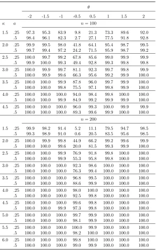
Table 1.12: Power of thefar test at θ0= 0, covariance setup 2.
θ
-2 -1.5 -1 -0.5 0.5 1 1.5 2
κ D n= 100
1.5 0.1 97.2 95.5 84.0 10.9 20.3 73.1 89.9 92.2
0.25 98.5 96.2 82.3 2.3 28.7 77.4 91.9 92.6
2.0 0.1 99.8 99.5 97.8 43.7 62.0 95.2 98.7 99.5
0.25 99.8 99.4 97.1 21.7 72.6 95.9 98.8 99.1
2.5 0.1 100.0 99.7 99.1 70.8 84.7 99.0 99.9 99.9
0.25 99.9 100.0 99.3 46.3 93.7 99.3 99.8 99.8
3.0 0.1 100.0 99.9 99.8 83.9 91.6 99.7 99.8 99.9
0.25 100.0 99.9 99.6 63.9 95.7 99.2 99.9 100.0
3.5 0.1 100.0 100.0 99.9 89.2 95.8 99.7 99.9 100.0
0.25 100.0 100.0 99.8 72.7 97.4 99.8 99.9 100.0
4.0 0.1 100.0 100.0 100.0 94.6 98.0 99.8 100.0 100.0
0.25 100.0 100.0 99.9 82.6 99.4 99.9 99.9 99.9
4.5 0.1 100.0 100.0 100.0 96.7 99.1 100.0 99.9 99.9
0.25 100.0 100.0 100.0 88.1 99.6 99.9 100.0 100.0
n= 200
1.5 0.1 99.9 98.1 91.5 5.2 10.7 79.5 94.7 98.5
0.25 99.4 98.9 90.2 0.4 24.8 84.8 95.4 98.4
2.0 0.1 100.0 99.9 99.8 45.7 65.9 99.2 99.6 99.9
0.25 100.0 100.0 99.6 13.9 85.1 99.6 99.9 100.0
2.5 0.1 100.0 100.0 99.9 77.4 91.8 99.8 100.0 100.0
0.25 100.0 100.0 99.9 45.0 96.3 99.8 100.0 100.0
3.0 0.1 100.0 100.0 100.0 92.4 98.6 100.0 100.0 100.0
0.25 100.0 100.0 100.0 65.8 99.5 100.0 100.0 100.0
3.5 0.1 100.0 100.0 100.0 97.0 99.5 100.0 100.0 100.0
0.25 100.0 100.0 100.0 82.2 99.9 100.0 100.0 100.0
4.0 0.1 100.0 100.0 100.0 98.0 100.0 100.0 100.0 100.0
0.25 100.0 100.0 100.0 88.6 99.9 100.0 100.0 100.0
4.5 0.1 100.0 100.0 100.0 99.6 99.8 100.0 100.0 100.0
0.25 100.0 100.0 99.9 94.1 99.9 100.0 100.0 100.0
5.0 0.1 100.0 100.0 100.0 99.8 99.9 100.0 100.0 100.0
0.25 100.0 100.0 100.0 95.8 99.9 100.0 100.0 100.0
5.5 0.1 100.0 100.0 100.0 100.0 99.9 100.0 100.0 100.0
0.25 100.0 100.0 100.0 96.3 100.0 100.0 100.0 100.0
6.0 0.1 100.0 100.0 100.0 99.9 100.0 100.0 100.0 100.0
0.25 100.0 100.0 100.0 97.8 99.9 100.0 100.0 100.0
Setup 2 corresponds tocov[ZW iuW i] =D. The corresponding correction factor for
Table 1.13: Power of thefar test at θ0= 0, covariance setup 3.
θ
-2 -1.5 -1 -0.5 0.5 1 1.5 2
κ a n= 100
1.5 .25 97.3 95.3 83.9 9.8 21.3 73.3 89.6 92.0
.5 98.4 96.1 82.3 2.7 27.1 77.5 91.8 92.8
2.0 .25 99.9 99.5 98.0 41.8 64.1 95.4 98.7 99.5
.5 99.7 99.4 97.2 24.2 71.5 95.9 98.7 99.2
2.5 .25 100.0 99.7 99.2 67.8 85.6 99.0 99.9 99.9
.5 99.9 100.0 99.3 49.4 92.8 99.3 99.8 99.8
3.0 .25 100.0 99.9 99.7 81.1 92.3 99.7 99.8 99.9
.5 100.0 99.9 99.6 66.3 95.6 99.2 99.9 100.0
3.5 .25 100.0 100.0 99.9 87.8 96.0 99.7 99.9 100.0
.5 100.0 100.0 99.8 75.5 97.1 99.8 99.9 100.0
4.0 .25 100.0 100.0 100.0 94.0 98.4 99.8 100.0 100.0
.5 100.0 100.0 99.9 84.9 99.2 99.9 99.9 100.0
4.5 .25 100.0 100.0 100.0 96.0 99.3 100.0 99.9 99.9
.5 100.0 100.0 100.0 89.3 99.6 99.9 100.0 100.0
n= 200
1.5 .25 99.9 98.2 91.4 5.2 11.1 79.5 94.7 98.5
.5 99.3 98.9 91.0 0.6 20.5 83.5 95.6 98.5
2.0 .25 100.0 99.9 99.8 44.9 66.2 99.2 99.6 99.9
.5 100.0 100.0 99.6 20.0 81.5 99.3 99.9 100.0
2.5 .25 100.0 100.0 99.9 76.9 91.8 99.8 100.0 100.0
.5 100.0 100.0 99.9 55.3 95.8 99.8 100.0 100.0
3.0 .25 100.0 100.0 100.0 92.3 98.6 100.0 100.0 100.0
.5 100.0 100.0 100.0 76.3 99.4 100.0 100.0 100.0
3.5 .25 100.0 100.0 100.0 96.8 99.5 100.0 100.0 100.0
.5 100.0 100.0 100.0 88.6 99.9 100.0 100.0 100.0
4.0 .25 100.0 100.0 100.0 98.0 100.0 100.0 100.0 100.0
.5 100.0 100.0 100.0 92.5 99.8 100.0 100.0 100.0
4.5 .25 100.0 100.0 100.0 99.6 99.8 100.0 100.0 100.0
.5 100.0 100.0 99.9 97.3 99.8 100.0 100.0 100.0
5.0 .25 100.0 100.0 100.0 99.7 99.9 100.0 100.0 100.0
.5 100.0 100.0 100.0 98.1 99.9 100.0 100.0 100.0
5.5 .25 100.0 100.0 100.0 100.0 99.9 100.0 100.0 100.0
.5 100.0 100.0 100.0 98.2 100.0 100.0 100.0 100.0
6.0 .25 100.0 100.0 100.0 99.8 100.0 100.0 100.0 100.0
.5 100.0 100.0 100.0 99.0 99.9 100.0 100.0 100.0
Setup 3 corresponds tocov[ZW iuW i] =an1/3/n1/2. The corresponding correction
1.8
References
Acemoglu, D., S. Johnson, and James A. Robinson (2001) “The Colonial Origins of Comparative Development: An Empirical Investigation,”American Economic Review, Vol. 91, pp. 1369–1401.
(2008) “Reply to the Revised (2008) version of David Albouy’s “The Colonial Origins of Comparative Development: An Investigation of the Settler Mortality Data,”.”
Acemoglu, Daron and Simon Johnson (2005) “Unbundling Institutions,” Journal of Political
Economy, Vol. 113, pp. 949–995.
Acemoglu, Daron, Simon Johnson, and James A. Robinson (2011) “Hither Thou Shalt Come, But No Further: Reply to “The Colonial Origins of Comparative Development: An Empirical Investigation: Comment”,” Working Paper 16966, National Bureau of Economic Research.
Albouy, David Y. (2008) “The Colonial Origins of Comparative Development: An Investigation of the Settler Mortality Data,” Working Papers series 14130, National Bureau of Economic Research, Inc.
Anderson, T. W. and H. Rubin (1949) “Estimation of the Parameters of a Single Equation in a Complete System of Stochastic Equations,” The Annals of Mathematical Statistics, Vol. 20, pp. 46–63.
Angrist, Joshua D (1990) “Lifetime Earnings and the Vietnam Era Draft Lottery: Evidence from Social Security Administrative Records,” American Economic Review, Vol. 80, pp. 313–336.
Berkowitz, Daniel, Mehmet Caner, and Ying Fang (2008) “Are “Nearly Exogenous Instruments” reliable?” Economics Letters, Vol. 101, pp. 20–23.
(2012) “The Validity of Instruments Revisited,” Journal of Econometrics, Vol. 166, pp. 255–266.
Caner, M. (2010) “Near Exogeneity and Weak Identification in Generalized Empirical Likelihood Estimators: Many Moment Asymptotics,” Working Paper, Department of Economics, North
Carolina State University.
Card, D. (1995) “Using Geographic Variation in College Proximity to Estimate the Returns to Schooling.,” In L.N. Christofides et al editors, Aspects of Labour Market Behaviour: Essays in
honor of John Vanderkamp. University of Toronto Press:, pp. 201–221.
Glaeser, Edward L., Rafael La Porta, Florencio Lopez de Silanes, and Andrei Shleifer (2004) “Do Institutions Cause Growth?” Journal of Economic Growth, Vol. 9, pp. 271–303.
Moreira, M. J. and B. P. Poi (2003) “Implementing Tests With Correct Size in the Simultaneous Equations Model,” Stata Journal, Vol. 3, pp. 57–70.
Riquelme, A., Berkowitz, D, and Caner, M. (2000) “Valid tests when instrumental variables do not perfectly satisfy the exclusion restriction,” Stata Journal, Vol. 13, pp. 528–546.
Stock, James H and Jonathan H Wright (2000) “GMM with weak identification,”Econometrica, Vol. 68, pp. 1055–1096.
Wooldridge, Jeffrey M. (2002) Econometric Analysis of Cross Section and Panel Data, Cam-bridge, MA: MIT Press.
*! V e r s i o n 1.0 J . A n d r e s R i q u e l m e 13 m a y 2 0 1 2
/* T h i s p r o g r a m p e r f o r m s t h e F r a c t i o n a l l y R e s a m p l e d A n d e r s o n R u b i n t e s t
( B e r k o w i t z , D . , Caner , M . a n d Y . Fang , 2 0 1 2 : T h e v a l i d i t y of i n s t r u m e n t s r e v i s i t e d . J o u r n a l of E c o n o m e t r i c s 166 , pp . 2 5 5 - 2 6 6 .
P r o g r a m m e d by : J . A n d r e s R i q u e l m e . P l e a s e s e n d a n y c o m m e n t to : j a r i q u e l @ n c s u . e d u */
c a p t u r e p r o g r a m d r o p far p r o g r a m d e f i n e far , r c l a s s
v e r s i o n 1 0 . 0
s y n t a x a n y t h i n g [ if ] [ in ] [ , r e p s ( i n t e g e r 1 0 0 0 0 ) k a p p a ( r e a l 3) t h e t a ( n u m l i s t ) ci l e v e l ( r e a l 95) G R i d ( n u m l i s t ) ]
l o c a l 0 ‘ a n y t h i n g ’
g e t t o k e n e x o g 0 : 0 , p a r s e ( " ( " ) g e t t o k e n d e p v a r e x o g : e x o g g e t t o k e n tmp 0 : 0 , p a r s e ( " ( " ) g e t t o k e n e n d o g 0 : 0 , p a r s e ( " = " ) g e t t o k e n tmp 0 : 0 , p a r s e ( " = " ) g e t t o k e n i n s t r 0 : 0 , p a r s e ( " ) " ) // B e g i n i n p u t c h e c k i n g < -// C h e c k if t h e r e a r e a n y c o n t r o l s
if ( w o r d c o u n t ( " ‘ exog ’ " ) == 0) l o c a l e x o g " " // i m m e d i a t e l y d e l e t e a n y b l a n k c h a r s // C h e c k f o r b e t a i n p u t ( no i n p u t m e a n s s i g n i f i c a n c e t e s t )
c a p t u r e m a t r i x d r o p _ _ t h e t a t e m p v a r _ t h e t a
l o c a l mm = w o r d c o u n t ( " ‘ endog ’ " )
m a t r i x _ _ t h e t a = J ( ‘ mm ’ , 1 , 0) // d e f a u l t if ( " ‘ theta ’ " != " " ) {
l o c a l bb = w o r d c o u n t ( " ‘ theta ’ " ) if ( ‘ mm ’ != ‘ bb ’) {
n o i s i l y : d i s p l a y " { e r r o r :{ bf : E R R O R -} { it : t h e t a () }: N u m b e r of g i v e n p a r a m e t e r s m u s t be e q u a l to the n u m b e r of e n d o g e n o u s v a r i a b l e s .} "
e r r o r ( 4 9 9 ) // c o d e 4 9 9 : g e n e r i c e r r o r }
f o r v a l u e s j = 1/ ‘ bb ’ {
l o c a l _a : w o r d ‘j ’ of ‘ theta ’ m a t r i x _ _ t h e t a [ ‘ j ’ , 1] = ‘ _a ’ }
}
// C h e c k C o n f i d e n c e i n t e r v a l i n p u t : if ( ‘ level ’ < 0 | ‘ level ’ > 1 0 0 ) {
n o i s i l y : d i s p l a y " { e r r o r :{ bf : E R R O R -} { it : l e v e l () }: C o n f i d e n c e l e v e l m u s t be b e t w e e n 0 and 1 0 0 . } "
e r r o r ( 4 9 9 ) // c o d e 4 9 9 : g e n e r i c e r r o r }
// C h e c k t h e " g r i d " // d e f a u l t g r i d : l o c a l g r _ l o w -30 l o c a l g r _ u p p 30 l o c a l g r _ i n c r = .01 if ( " ‘ grid ’ " != " " ) {
if ( w o r d c o u n t ( " ‘ grid ’ " ) != 3) {
n o i s i l y : d i s p l a y " { e r r o r :{ bf : E R R O R -} { it : g r i d () }: G r i d o p t i o n r e q u i r e s 3 i n p u t s .} "
e r r o r ( 4 9 9 ) // c o d e 4 9 9 : g e n e r i c e r r o r }
l o c a l g r _ l o w : w o r d 1 of ‘ grid ’ l o c a l g r _ u p p : w o r d 2 of ‘ grid ’ l o c a l g r _ i n c r : w o r d 3 of ‘ grid ’ if ( ‘ gr_low ’ >= ‘ gr_upp ’ ) {
n o i s i l y : d i s p l a y " { e r r o r :{ bf : E R R O R -} { it : g r i d () }: L o w e r l i m i t m u s t be l o w e r t h a n u p p e r l i m i t .} "
e r r o r ( 4 9 9 ) // c o d e 4 9 9 : g e n e r i c e r r o r }
n o i s i l y : d i s p l a y " { e r r o r :{ bf : E R R O R -} { it : g r i d () }: I n c r e m e n t m u s t be a p o s i t i v e i n t e g e r .} "
e r r o r ( 4 9 9 ) // c o d e 4 9 9 : g e n e r i c e r r o r }
}
if ( " ‘ ci ’ " != " " & w o r d c o u n t ( " ‘ theta ’ " ) > 1) {
n o i s i l y : d i s p l a y " { e r r o r :{ bf : E R R O R -} { it : ci }: C o n f i d e n c e I n t e r v a l o p t i o n v a l i d o n l y w i t h one (1) e n d o g e n o u s v a r i a b l e .} "
e r r o r ( 4 9 9 ) // c o d e 4 9 9 : g e n e r i c e r r o r }
// C h e c k t h e n u m b e r of r e p e t i t i o n s : if ‘ reps ’ <= 0 {
n o i s i l y : d i s p l a y " { e r r o r :{ bf : E R R O R -} { it : r e p s () } m u s t be a p o s i t i v e i n t e g e r .} " e r r o r ( 4 9 9 ) // c o d e 4 9 9 : g e n e r i c e r r o r
}
// C h e c k t h e k a p p a v a l u e : if ( ‘ kappa ’ < 0 ) {
n o i s i l y : d i s p l a y " { e r r o r :{ bf : E R R O R -} { it : k a p p a } out of range , it has to be a p o s i t i v e n u m b e r .} "
e r r o r ( 4 9 9 ) // c o d e 4 9 9 : g e n e r i c e r r o r }
// - - - > E n d I n p u t C h e c k i n g m a r k s a m p l e t o u s e
m a t a : f a r _ 1 ( " ‘ depvar ’ " , " ‘ exog ’ " , " ‘ endog ’ " , " ‘ instr ’ " , " ‘ touse ’ " , ‘ reps ’ , ‘ kappa ’ , // /
" ‘ ci ’ " , ‘ level ’ , ‘ gr_low ’ , ‘ gr_upp ’ , ‘ gr_incr ’ ) // s e n d v a r s to m a t a
// O u t p u t p r e p a r a t i o n a n d d i s p l a y .
l o c a l t i t l e " F r a c t i o n a l l y r e s a m p l e d A n d e r s o n and R u b i n t e s t " l o c a l n_ : d i s p l a y % 7 . 0 f ‘ r ( N ) ’
l o c a l f a r p _ : d i s p l a y % 9 . 4 f ‘ r ( F A R p ) ’ l o c a l a r p _ : d i s p l a y % 9 . 4 f ‘ r ( ARp ) ’ l o c a l ar_ : d i s p l a y % 9 . 4 f ‘ r ( AR ) ’ l o c a l r e p s _ : d i s p l a y % 9 . 0 f ‘ r ( R E P S ) ’ d i s p l a y " "
d i s p l a y " { i n p u t : ‘ title ’.} "
d i s p l a y " { h l i n e 1 5 } { c TT }{ h l i n e 60} "
d i s p l a y " { i n p u t : { c |} F u l l s a m p l e F u l l s a m p l e FAR } "
d i s p l a y " { i n p u t : { c |} s t a t i s t i c p - v a l u e p - v a l u e r e p s N } "
d i s p l a y " { h l i n e 1 5 } { c +}{ h l i n e 60} "
d i s p l a y " { i n p u t : AR - t e s t { c |}} { r e s u l t : ‘ ar_ ’} { r e s u l t : ‘ arp_ ’} { r e s u l t : ‘ farp_ ’} { r e s u l t : ‘ reps_ ’} { r e s u l t : ‘ n_ ’} "
d i s p l a y " { h l i n e 1 5 } { c BT }{ h l i n e 60} " r e t u r n s c a l a r l e v e l = ‘ level ’
r e t u r n s c a l a r n = r ( N ) r e t u r n s c a l a r m = r ( M ) r e t u r n s c a l a r l = r ( L ) r e t u r n s c a l a r k = r ( K )
r e t u r n s c a l a r k a p p a = r ( k a p p a ) r e t u r n s c a l a r r e p s = r ( R E P S ) r e t u r n s c a l a r f a r p = r ( F A R p ) r e t u r n s c a l a r arp = r ( ARp ) r e t u r n s c a l a r ar = r ( AR )
if ( ‘ reps ’ != 1 0 0 0 | ‘ kappa ’ != 3 | " ‘ theta ’ " != " " | ‘ level ’ != 95 | " ‘ ci ’ " != " " | " ‘ grid ’ " != " " ) l o c a l o p t c " , "
if ( ‘ reps ’ != 1 0 0 0 ) l o c a l o p t r " r e p s ( ‘ reps ’) " if ( ‘ kappa ’ != 3) l o c a l o p t k " c ( ‘ kappa ’) " if ( " ‘ theta ’ " != " " ) l o c a l o p t b " t h e t a ( ‘ theta ’) " if ( ‘ level ’ != 95 ) l o c a l o p t l " l e v e l ( ‘ level ’) "
if ( " ‘ grid ’ " != " " ) l o c a l o p t g " g r i d ( ‘ gr_low ’ , ‘ gr_upp ’ , ‘ gr_incr ’) " r e t u r n l o c a l g r i d ‘ grid ’
r e t u r n l o c a l c m d l i n e " far ‘ a n y t h i n g ’ ‘ if ’ ‘ in ’ ‘ optc ’ ‘ optr ’ ‘ optk ’ ‘ optb ’ ‘ ci ’ ‘ optl ’ ‘ optg ’ "
r e t u r n l o c a l t i t l e ‘ title ’ r e t u r n m a t r i x t h e t a _ _ t h e t a
m a t r i x c o l n a m e s rci = t h e t a FAR - p t e s t r e t u r n m a t r i x ci rci
end
c a p t u r e m a t a m a t a d r o p f a r _ 1 () m a t a
v o i d f a r _ 1 ( s t r i n g s c a l a r depvar , s t r i n g s c a l a r exog , s t r i n g s c a l a r endog , // / s t r i n g s c a l a r instr , s t r i n g s c a l a r touse , // /
r e a l nb , r e a l kappa , s t r i n g s c a l a r ci , r e a l level , r e a l gr_low , r e a l gr_upp , r e a l g r _ i n c r )
{
r e a l m a t r i x M , Y , Z , W r e a l c o l v e c t o r y
r e a l s c a l a r n , m , ar , far M = Y = Z = W = y =.
t h e t a = s t _ m a t r i x ( " _ _ t h e t a " )
s t _ v i e w ( y , . , t o k e n s ( d e p v a r ) , t o u s e ) if ( e x o g != " " ) {
s t _ v i e w ( W , . , t o k e n s ( e x o g ) , t o u s e ) }
e l s e {
W = J ( r o w s ( y ) ,1 ,1) // d u m m y s i n g l e c o l u m n to c h e c k f o r m i s s i n g s }
s t _ v i e w ( Y , . , t o k e n s ( e n d o g ) , t o u s e ) s t _ v i e w ( Z , . , t o k e n s ( i n s t r ) , t o u s e ) // E l i m i n a t e m i s s i n g v a l u e s f r o m t h e s a m p l e
M = y , W , Y , Z t f i l t e r = 1:: r o w s ( M )
for ( i =1; i <= r o w s ( M ) ; i ++) { for ( j =1; j <= c o l s ( M ) ; j ++) {
if (!( M [ i , j ] <.) ) t f i l t e r [ i ] = . }
}
f i l t e r = min ( t f i l t e r )
for ( k = min ( f i l t e r ) +1; k <= r o w s ( t f i l t e r ) ; k ++) {
if ( t f i l t e r [ k ,1] != .) f i l t e r = f i l t e r \ t f i l t e r [ k ,1] }
f i l t e r = filter ’ n = l e n g t h ( f i l t e r )
M = M [( f i l t e r ) , 1.. c o l s ( M ) ] y = y [( f i l t e r ) , 1.. c o l s ( y ) ] // G e t t h e E n d o g e n o u s
Y = Y [( f i l t e r ) , 1.. c o l s ( Y ) ]
m = c o l s ( Y ) // m : n u m b e r of e n d o g e n o u s // C h e c k c o l l i n e a r i t y : e n d o g e n o u s
if ( r a n k ( Y ) < m ) {
e r r p r i n t f ( " E r r o r : C o l l i n e a r e n d o g e n o u s v a r i a b l e s \ n " ) e x i t ( 4 9 9 )
}
// G e t t h e C o n t r o l s
if ( e x o g == " " ) W = J ( n ,1 ,1) // no c o n t r o l s
if ( e x o g != " " ) W = J ( n ,1 ,1) , W [( f i l t e r ) , 1.. c o l s ( W ) ] // c o n t r o l s l = c o l s ( W ) // l : n u m b e r of c o n t r o l s
// C h e c k f o r c o l l i n e a r i t y : c o n t r o l s if ( e x o g != " " & r a n k ( W ) < l ) {
e r r p r i n t f ( " E r r o r : C o l l i n e a r c o n t r o l s \ n " ) e x i t ( 4 9 9 )
}
// G e t t h e I n s t r u m e n t s
Z = Z [( f i l t e r ) , 1.. c o l s ( Z ) ]
k = c o l s ( Z ) // k : n u m b e r of i n s t r u m e n t s // C h e c k f o r c o l l i n e a r i t y : i n s t r u m e n t s
if ( r a n k ( Z ) < k ) {
e x i t ( 4 9 9 ) }
// P r o j e c t o u t c o n t r o l s
P = W * i n v s y m ( W ’* W ) * W ’ // P r o j e c t i o n m a t r i x Yw = Y - P * Y
yw = y - P * y Zw = Z - P * Z
// E s t i m a t e s w i t h o u t c o n f i d e n c e i n t e r v a l
r e s u l t s = f a r _ 2 ( yw , Yw , Zw , n , m , kappa , nb , t h e t a ) ar = r e s u l t s [1]
arp = r e s u l t s [2] f a r p = r e s u l t s [3]
// E x p o r t r e s u l t s to m a i n r o u t i n e s t _ r c l e a r ()
s t _ n u m s c a l a r ( " r ( N ) " , n ) s t _ n u m s c a l a r ( " r ( L ) " , l ) s t _ n u m s c a l a r ( " r ( M ) " , m ) s t _ n u m s c a l a r ( " r ( K ) " , k ) s t _ n u m s c a l a r ( " r ( AR ) " , ar ) s t _ n u m s c a l a r ( " r ( F A R p ) " , f a r p ) s t _ n u m s c a l a r ( " r ( ARp ) " , arp ) s t _ n u m s c a l a r ( " r ( R E P S ) " , nb ) s t _ n u m s c a l a r ( " r ( k a p p a ) " , k a p p a ) // C o n f i d e n c e i n t e r v a l
g r i d = ( t h e t a [1 ,1] , farp , farp >= l e v e l / 1 0 0 ) if ( ci != " " ) {
g r i d = r a n g e ( gr_low , gr_upp , g r _ i n c r )
g r i d = g r i d , J ( r o w s ( g r i d ) , 2 ,0) // M a k e t h e g r i d a n d r e s u l t s for ( k =1; k <= r o w s ( g r i d ) ; k ++) {
r e s u l t s = f a r _ 2 ( yw , Yw , Zw , n , m , kappa , nb , g r i d [ k , 1 ] ) g r i d [ k ,2] = r e s u l t s [3]
g r i d [ k ,3] = g r i d [ k ,2] >= (100 - l e v e l ) / 1 0 0 } }
s t _ m a t r i x ( " rci " , g r i d ) }
end
c a p t u r e m a t a m a t a d r o p f a r _ 2 () m a t a
f u n c t i o n f a r _ 2 ( r e a l m a t r i x yw , r e a l m a t r i x Yw , r e a l m a t r i x Zw , // / r e a l n , r e a l m , r e a l kappa , r e a l nb , r e a l m a t r i x b0 )
{
// F u l l S a m p l e H e t e r o s k e d a s t i c i t y r o b u s t A n d e r s o n R u b i n T e s t err = Zw :*( yw - Yw * b0 ) // S t r u c t u r a l e r r o r
vc = ( err ’* err ) / n // E s t i m a t e d c o v a r i a n c e m a t r i x
ar = (( yw - Yw * b0 ) ’* Zw * i n v s y m ( vc ) * Zw ’*( yw - Yw * b0 ) ) / n // H e t . r o b u s t A n d e r s o n R u b i n t e s t // F A R v a l u e s
f = 1/2 - k a p p a / s q r t ( n ) // F r a c t i o n of o r i g i n a l s a m p l e to be r e s a m p l e d b = c e i l ( n * f ) // B l o c k s i z e
f = b / n
arb = J ( nb ,1 ,0) // A n d e r s o n - R u b i n t e s t m a t r i x pre - a l l o c a t i o n for ( i =1; i <= nb ; i ++) {
blq = J ( b ,1 ,0)
r1 = c e i l (( n :: n - b +1) :* u n i f o r m ( b ,1) ) + ( 0 : : b -1) // R a n d o m s a m p l e ( w i t h r e p e t i t i o n ) r2 = 1:: n
for ( h =1; h < b ; h ++) {
r2 [( h , r1 [ h ]) ] = r2 [( r1 [ h ] , h ) ] // R a n d o m r e s a m p l i n g }
blq = r2 [ ( 1 . . b ) ,1] // R a n d o m r e s a m p l e ( no r e p e t i t i o n ) e r r 2 = yw - Yw * b0
arb [ i ] = ( b /(1 - f ) ) *(( e r r 2 [ blq ] ’* Zw [ blq , . ] ) / b ) * i n v s y m ( vc ) *(( Zw [ blq ,.] ’* e r r 2 [ blq ]) / b ) }
arb = s o r t ( arb ,1)
arp = 1 - c h i 2 ( m , ar ) // A n d e r s o n - R u b i n p v a l u e e s t i m a t e
f a r p = m e a n ( ar : <= arb ) // R e s a m p l e d A n d e r s o n R u b i n p v a l u e e s t i m a t e r e t u r n ( ar , arp , f a r p )
C h a p t e r 2 : M o m e n t a n d I V S e l e c t i o n A p p r o a c h e s : A
C o m pa r at i v e S i m u l at i o n S t u d y
2.1
Preliminaries
The focus of the first chapter was the problem of the inference when the instrumental variables
do not that perfectly satisfy the exclusion restriction, but are still used because of the difficulty
of finding alternative ones. The underlying problem was that the best the researcher could do
was work with a set of imperfect instruments. In this chapter a different but related problem
is addressed: when the researcher has a large –and probably diverging– number of candidate
instruments and only some of them are valid, two concerns arise: (1) the inclusion of invalid
instruments generate bias in the estimations, and (2) it is know the fact thatgmm estimators
have poor finite sample properties in highly overidentified models. Under this circumstances,
the relevant question is how to pick up the valid instruments and discard the invalid ones? We
refer to this issue as the moment selection problem, which may be adjudicated statistically with
the J-test which indicates whether overidentified restrictions are valid. If the null hypothesis is
rejected, the researcher would need to employ a moment selection criteria (msc) that would
allow distinguishing between the valid and invalid moment conditions.
we focus on information-based methods and review three of the moment selection criteria used in
the current literature: (i) the shrinkage procedure as in Liao (2013), (ii) the information-based
criteria with gmmin Andrews (1999), and (iii) the information based criterion using generalized
empirical likelihood of Hong, Preston and Shum (2003).
The main objective of this chapter is to compare the aforementioned msc in a fairly
comprehensive manner. By using Monte Carlo simulations we compare these methods in their
performance in selecting valid moments in linear settings under several relevant scenarios: small
and large sample sizes, fixed and increasing number of moment conditions, weak and strong
identification, local-to-zero moment conditions, homoskedastic and heteroskedastic errors. We
also analyze the second stage estimation performance of each msc by considering the finite
sample properties of structural parameter estimators. To this end, we employ Okui (2011)
model averaging technique to get better Mean Squared Error, and smaller bias for the structural
parameters. We find that the Adaptive Lasso in the model selection stage, coupled with either
unpenalized gmmor moment averaging of Okui delivers generally the smallest rmse for the
second stage coefficient estimators.
2.2
Introduction
It is not uncommon to encounter a large number of instruments or moment conditions in
the applications of instrumental variables (iv) or the Generalized Method of Moments (gmm)
estimators. Some ivs or moments may be invalid, but the researcher does not know a priori
which ones. This problem may be adjudicated statistically with the J-test which indicates
whether overidentified restrictions are valid. If the null is rejected, the researcher would need
to a moment selection technique that would allow distinguishing between the valid and invalid
moment conditions. A few techniques have been proposed, each one with advantages (for