Proposed Algorithms to solve Big Data traveling
salesman problem
Mohammed Ahmed Alhanjouri
1
Computer Engineering Department, Islamic University of Gaza, Gaza, Palestine
Abstract
Big data is one of the most concerned topics in business today across information technology sectors. most research fields toward using big data tools to leverage from the huge data that available today.
The traveling salesman problem is one of problems that is growth by increasing the input as a factorial (n!). therefore it is important to find algorithm to solve big number of cities with feasible time and within available memory space.
This article introduces two proposed algorithms to solve traveling salesman problem by clustering using three methods; k-means, Gaussian Mixture Model, and Self-Organizing Map to select the best one for proposed algorithms.
The proposed algorithms depend on arranging the cities (points) in chromosomes for Genetic Algorithm after clustering the big data to reduce the problem and solving each cluster separately based on divide and conquer concept.
The two proposed algorithms tested by applying on different number of points, the nearest points algorithm solved traveling salesman problem with 2 million points.
Keywords: Big Data Clustering, traveling salesman problem, k-means, Gaussian Mixture Model, and Self-Organizing Map
1. Introduction
Big data can be described as massive amounts of public data generated on a daily basis, or it is described by some data scientists as tsunami of data. [1]. The data volume is increasing exponentially due to rapid changes. Companies such as Facebook, Google, Twitter, Yahoo, Microsoft and Amazon routinely deal with petabytes of data on a daily basis. It’s estimated that we are generating an incredible 2.5 quintillion bytes per day.
Big Data is often described as data that are too large to process or analyze on a regular computer with common tools like the popular spreadsheet application Microsoft Excel. Big data is relative to the computing power at our fingertips [2].
“Big data refers to datasets whose size is beyond the ability of typical database software tools to capture, store, manage, and analyze. This definition is intentionally subjective and incorporates a moving definition of how big a dataset needs to be in order to be considered big data—i.e., we don’t define big data in terms of being larger than a certain
number of terabytes (thousands of gigabytes). We assume that, as technology advances over time, the size of datasets that qualify as big data will also increase. Also note that the definition can vary by sector, depending on what kinds of software tools are commonly available and what sizes of datasets are common in a particular industry. With those caveats, big data in many sectors today will range from a few dozen terabytes to multiple petabytes (thousands of terabytes).” [3].
2. Traveling Salesman Problem (TSP)
The idea of the traveling salesman problem (TSP) is to find a tour of a given number of cities, visiting each city exactly once and returning to the starting city where the length of this tour is minimized.
The first instance of the traveling salesman problem was from Euler in 1759 whose problem was to move a knight to every position on a chess board exactly once [4]. The traveling salesman first gained fame in a book written by German salesman BF Voigt in 1832 on how to be a successful traveling salesman [4]. He mentions the TSP, although not by that name, by suggesting that to cover as many locations as possible without visiting any location twice is the most important aspect of the scheduling of a tour.
The origins of the TSP in mathematics are not really known all we know for certain is that it happened around 1931.
The standard or symmetric traveling salesman problem can be stated mathematically as follows:
Given a weighted graph G = (V, E) where the weight cij on the edge between nodes i and j is a non-negative value, find the tour of all nodes that has the minimum total cost or distance.
in this work we will examine some of modern optimization techniques to solve the problem within feasible time. Mathematically, A Travelling Salesman Problem (TSP) can be defined on a graph G = (V, E) where V is a vector of cities {1,2,....,n} where n is the number of cities .Then,
E = {(i,j): i,j ∈ V, i≠j } is an edge set. A cost matrix C = (cij) is defined on E. In particular, this is the case of planar
problems for which the vertices are points Pi = (Xi, Yi) and Pj = (Xj, Yj). So, cij =
is distance between these points. So, the problem could be formalized as: Minimize f(x) = , to satisfy our goal to find the minimum total distance of each chromosome was populated, where visiting each city exactly once and returning back to the starting city. That computed f(x) was presented a fitness function in used techniques [5].
Many different methods of optimization have been used to try to solve the TSP. Homaifar [6] states that “one approach which would certainly find the optimal solution of any TSP is the application of exhaustive enumeration and evaluation. The procedure consists of generating all possible tours and evaluating their corresponding tour length. The tour with the smallest length is selected as the best, which is guaranteed to be optimal. If we could identify and evaluate one tour per nanosecond (or one billion tours per second), it would require almost ten million years (number of possible tours = 3.2×10²³) to evaluate all of the tours in a 25 city TSP.”
Obviously we need to find an algorithm that will give us a solution in a shorter amount of time. As we said before, the traveling salesman problem is NP-hard so there is no known algorithm that will solve it in polynomial time. We will probably have to sacrifice optimality in order to get a good answer in a shorter time. Many algorithms have been tried for the traveling salesman problem.
Greedy Algorithms [7] are a method of finding a feasible solution to the traveling salesman problem however they are not always good.
The Nearest Neighbor [7] algorithm is similar to the greedy algorithm in its simple approach. This algorithm also does not always give good solutions.
A minimum spanning tree [8] is a set of n−1 edges (where again n is the number of cities) that connect all cities so that the sum of all the edges used is minimized.
TSP is a minimization problem; we consider f(x) as a fitness function, where f(x) calculates cost (or value) of the tour between cities (nodes).
Many optimization algorithms are used to solve TSP such as in [9] they used Ant Colony and compared it with GA. Alhanjouri [5] applied six optimization algorithms;
Genetic Algorithm (GA), Simulated Annealing (SA), Particle Swarm Optimization (PSO), Ant Colony Optimization (ACO), Bacteria Foraging Optimization (BFO), and Bee Colony Optimization (BCO) to achieve comparative study to solve TSP with different sizes up to 14051 cities which spent a lot of time to find results by three algorithms while other three are failed, to solve that we need to reduce the computation time and space.
Many techniques are improved to introduce Clustering TSP (CTSP), but few ones that concerned the big data such as in [10] that introduced adaptive resonance theory (ART) to solve a one million points TSP.
3. Clustering Methods
This work introduces proposed algorithm to solve TSP by clustering of big data. The clustering used methods in this work are k-means, Gaussian Mixture Model (GMM), and Self Organizing Map (SOM).
3.1 k-means
K-means clustering is a type of unsupervised learning, which is used when you have unlabeled data (i.e., data without defined categories or groups). The goal of this algorithm is to find groups in the data, with the number of groups represented by the variable K. The algorithm works iteratively to assign each data point to one of K groups based on the features that are provided. Data points are clustered based on feature similarity. The results of the K-means clustering algorithm are:
1. The centroids of the K clusters, which can be used to label new data
2. Labels for the training data (each data point is assigned to a single cluster)
Rather than defining groups before looking at the data, clustering allows you to find and analyze the groups that have formed organically. The "Choosing K" section below describes how the number of groups can be determined. Each centroid of a cluster is a collection of feature values which define the resulting groups. Examining the centroid feature weights can be used to qualitatively interpret what kind of group each cluster represents [11 ].
either be randomly generated or randomly selected from the data set. The algorithm then iterates between two steps:
1. Data assignment step:
Each centroid defines one of the clusters. In this step, each data point is assigned to its nearest centroid, based on the squared Euclidean distance. More formally, if ci is the collection of centroids in set C, then each data point x is assigned to a cluster based on
(1)
Where dist( · ) is the standard (L2) Euclidean distance. Let the set of data point assignments for each ith cluster centroid be Si.
2. Centroid update step:
In this step, the centroids are recomputed. This is done by taking the mean of all data points assigned to that centroid's cluster.
(2)
The algorithm iterates between steps one and two until a stopping criteria is met (i.e., no data points change clusters, the sum of the distances is minimized, or some maximum number of iterations is reached).
This algorithm is guaranteed to converge to a result. The result may be a local optimum (i.e. not necessarily the best possible outcome), meaning that assessing more than one run of the algorithm with randomized starting centroids may give a better outcome.
This algorithm finds the clusters and data set labels for a particular pre-chosen K. To find the number of clusters in the data, the user needs to run the K-means clustering algorithm for a range of K values and compare the results. In general, there is no method for determining exact value of K, but an accurate estimate can be obtained using the following techniques.
One of the metrics that is commonly used to compare results across different values of K is the mean distance between data points and their cluster centroid. Since increasing the number of clusters will always reduce the distance to data points, increasing K will always decrease this metric, to the extreme of reaching zero when K is the same as the number of data points. Thus, this metric cannot
be used as the sole target. Instead, mean distance to the centroid as a function of K is plotted and the "elbow point," where the rate of decrease sharply shifts, can be used to roughly determine K.
A number of other techniques exist for validating K, including cross-validation, information criteria, the information theoretic jump method, the silhouette method, and the G-means algorithm. In addition, monitoring the distribution of data points across groups provides insight into how the algorithm is splitting the data for each K. For CTSP we don’t care about K, because this application is not data which need to be accurate separated. Thus K can be chosen according to size of data (No. of cities) to reduce the time complexity as possible. To achieve that, we chose K as root of No. of cities ( ).
3.2 Gaussian mixture model
Let us assume that components of the mixture have Gaussian distribution with mean μ and variance σ2 and probability density function (Equation 3). The choice of the Gaussian distribution is natural and very common when we deal with a natural object or phenomenon, such as sand. But the mixture model approach can be applied to the other distributions from the exponential family.
(3)
We let o1,o2,...,oL denote our observations or data points. Then each data point is assumed to be an independent realization of the random variable O with the three-component mixture probability density function and log-likelihood function as showm in Equations (4 and 5) respectively. With the maximum likelihood approach to the estimation of our model
M = 〈ν, N (μ1, σ1),..., N(μK, σK)〉 , we need to find such values of νi, μi and σi that maximize the function (2.3). To solve the problem, the Expectation Maximization (EM) Algorithm is used.
point oi belongs to the j-th mixture component. All weights for a given data point must sum to one as in Equation (6).
(6) For each iteration, we use the current parameters of the model to calculate weights for all data point (expectation step or E-step), and then we use these updated weights to recalculate parameters of the model (maximization step or M-step). Let us see how the EM algorithm works in some details. First, we have to provide an initial approximation of model M(0) using one of the following ways:
(1) Partitioning data points arbitrarily among the mixture components and then calculating the parameters of the model.
(2) Setting up the parameters randomly or based on our knowledge about the problem.
After this, we start to iterate E- and M-steps until a stopping criterion gets true. For the E-step the expected component membership weights are calculated for each data point based on parameters of the current model [McLachlan]. This is done using the Bayes’ Rule that calculates the weight wij as the posterior probability of membership of i-th data point in j-th mixture component (Equation 7).
(7) For the M-step, the parameters of the model are recalculated using Equations (8), (9) and (10), based on our refined knowledge about membership of data points.
A good feature of the EM algorithm is that the likelihood function in Equation (5) can never decrease; hence it eventually converges to a local maximum. In practice, the algorithm stops when the difference between two consecutive values of likelihood function is less than a threshold as described in Equation (11).
(11) The mixture model approach and the EM algorithm have been generalized to accommodate multivariate data and other kind of probability distributions. Another method of generalization is to split multivariate data into several sets
or streams and create a mixture model for each stream, but have the joint likelihood function [12].
The special feature of mixture models is that they work in cases when the components are heavily intersected.
3.3 Self-Organizing Map (SOM)
SOM is a neural network model which is an unsupervised learning algorithm used to obtain a topology-preserving mapping from the (usually high dimensional) input/feature space to an output/map space of fewer dimensions (in TSP case is 2D).
SOMs have two phases; Learning phase by built map, that represents the input dimensions and output number of clusters, network organized using a competitive process applied on training set. Prediction phase, new vectors are quickly given a location on the converged map, easily classifying or categorizing the new data [13].
SOM learning phase can be summarized as: 1) Initialize each node’s weights.
2) Choose a random vector from training data and present it to the SOM.
3) Find the best matching unit by calculating the distance between the input vector (V1, V2, ... , Vn) and the weights (W1, W2, ... , Wn) of each node as 4) Each node in the best matching unit has its weights
adjusted to become more like the best matching unit. Nodes closest to the best matching unit are altered more than the nodes furthest away in the neighborhood. 5) Repeat from step 2 for enough iterations for
convergence.
4. Proposed Algorithms
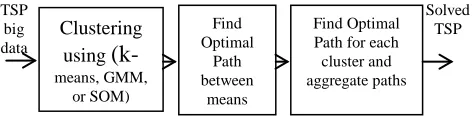
In this section, two proposed algorithm were implemented with small change but large effect. In general Figure (1) describe the whole systems that includes clustering method (k-means, Gaussian mixture model, or SOM neural network), solving TSP for produced means, then solving TSP for each cluster and aggregate them.
Clustering using
(k-means, GMM, or SOM)
Find Optimal
Path between
means
Find Optimal Path for each cluster and aggregate paths TSP
big data
Solved TSP
Figure 1. General clustering method for TSP
(8)
(9)
Both two proposed algorithms associates the two first blocks in Figure (1), but the difference will be appears in last one to solve whole combination of clusters points. In both algorithms, all huge number of points will be clustering to extract √n means. This number of cluster achieving the smallest number of points in each cluster which need to be solved by GA as a factorial complexity O(n!). For example, one million of points can be divided into 1000 clusters, in each one about 1000 point as an average. For uniform distributed points will be ideally 1000 points, but in case of non-uniform distributed points, some clusters will need more time to find the optimal path while other clusters will need less time.
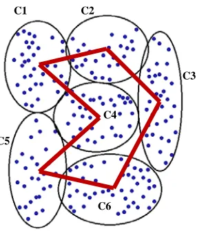
These means will be solved as TSP to find the best path between means. Figure (2) shows random 200 points to explain the proposed algorithms that will be clustered as shown in six clusters with six means extracted by k-means, GMM, or SOM clustering method, also the best path between means as illustrated.
4.1 First proposed algorithm: nearest points
After finding the best path between means, we need to find the best path between the points for each individual cluster. The first proposed algorithm to find best path is determining the start and end (terminal) points in each cluster to be connected with another cluster. Figure (3) illustrates the terminal two points in C5 which lied between C4 and C6 as in Figure (2), first point in C5 is calculated as the nearest point to the mean of C4, and the second one in C5 is calculated as the nearest point to the mean of C6 as shown in Figure (3). All terminals for all clusters are calculated to connect each pair together according to the best path between clusters in Figure (2).
To solve TSP for each cluster, we arranging the chromosomes in GA as in Figure (4), the terminal points should be always in terminals genes (first and last nodes)
The first and last genes were not changed during GA generations, while the other genes that represent cities will be changed according to crossover and mutation processes. After find the best path for each cluster, these paths will connected together according to terminal points and the best path between clusters to produce Figure (5) as the result for whole first system.
C1 C2
C3
C4
C5
C6
Fig. 2 Clustering results and the best path between clusters for 200 random TSP points
Fig. 3. Determining the nearest point to adjust cluster
1 3 2
1- First terminal point in cluster 2- Second terminal point in cluster 3- Other points in cluster
Figure 4, arrangement of chromosomes to solve TSP for each cluster
4.2 Second proposed algorithm: combinatorial
clustering
In this algorithm, all clusters points will be solved together by ordering the clusters sequentially according to best path between clusters as shown if Figure (6)
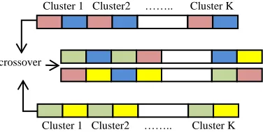
The points of cluster 1 comes firstly in chromosome then followed by the points of cluster 2 and so on to finish with the points of cluster K (last one). To achieve GA for this concatenated chromosome the processes (crossover, and mutation) are accomplished as in Figure (7) that apply GA processes for each cluster to generate the next generation, i.e. cluster by cluster. The mutation can be achieved by swapping two points in cluster.
Figure (8) illustrates an example solving 200 points TSP. the first step is clustering that produced six clusters, then solving TSP for 6-means to find the best path as appear by bold lines. The next step is constructing population size of chromosomes initialized by clustering results as in Figure (6) and apply GA as in Figure (7) to solve whole TSP.
5. Experimental Results
In this part, the results for three clustering methods which combined with our two proposed algorithms are viewed. The results obtained by using HP i7 workstation desktop with specifications:
Memory 128 GB DDR4 Windows 10 Pro 64,
Intel® Xeon® E5-1660 v4 (3.2 GHz, 20 MB cache, 8 cores, Intel® vPro™)
Graphics card NVIDIA® Quadro® M4000 (8 GB) HD 500GB SSD
The proposed algorithms are tested on random huge number of points to achieve our target to solve big data traveling salesman problem. The programs are written on Matlab without using GA toolbox which doesn't give us the abilities to state the terminals or to arrange the points according to their cluster.
Table (1) shows the comparison between clustering methods based on tour and computation time for two proposed algorithms by using 2000 random points. Population size is 150 chromosomes, number of generations is 100, crossover probability is 0.7, and mutation probability is 0.01.
Table 1: Comparison of used clustering methods Clustering
Method
Proposed Algorithm
Total tour
Computational time (S)
k-means First 4981 83 Second 4980 163
GMM First 4979 137
Second 4987 194
SOM First 4980 105
Second 4987 145 First = nearest points algorithm
Second = combinatorial clustering algorithm
From Table (1) we can extract some important notes to complete out results toward big data. Firstly the best tour achieved by GMM but with dramatically increasing in computational time versus k-means because that the computations in k-means is simple comparing with GMM and SOM, and the tour length is close to the best one. therefore k-means is more suitable to complete this work toward big data and compare between the two proposed algorithms.
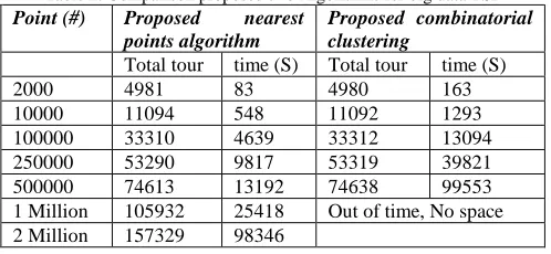
The next experimental results are to test the proposed algorithms by using k-means on big date that gradually increased to reach 1 Million points as shown in Table (2). As shown in Table (2), Proposed nearest points algorithm is better than Proposed combinatorial clustering in both total tour length and computational time for big data. For more than 500,000 points, proposed combinatorial
Cluster 1 Cluster2 …….. Cluster K
Fig. 6 ordering chromosome of all points according to best path of all clusters
Fig. 8 the resultant best path using combinatorial clustering algorithm Fig. 7 GA processes for each cluster to generate the next generation
Cluster 1 Cluster2 …….. Cluster K
crossover
clustering is stopped because it needs more time and memory space, while nearest points algorithm doesn't need it. For example if we have a one million uniform distributed points, then about 1000 clusters are classified. In nearest points algorithm, we find the solution for each cluster separately, with (1000!) possible solutions will repeated 1000 times without more space, solution of cluster will be estimated and saved before starting another cluster, and finally recall all solutions to connect the nearest points between clusters. But for the same problem, the combinatorial clustering needs to combine all clusters points in one chromosome to create (1,000,000!) possible solutions, the probability to find solution will be reduced beside to need more time to reach acceptable solution.
Table 2: Comparison proposed two Algorithms for big data TSP
Point (#) Proposed nearest
points algorithm
Proposed combinatorial clustering
Total tour time (S) Total tour time (S)
2000 4981 83 4980 163
10000 11094 548 11092 1293
100000 33310 4639 33312 13094
250000 53290 9817 53319 39821
500000 74613 13192 74638 99553 1 Million 105932 25418 Out of time, No space 2 Million 157329 98346
6. Conclusion
This work introduced proposed nearest points algorithm as a new techniques to solve TSP and its applications for big data reach to two millions nodes. The proposed algorithm compared with the
combinatorial clustering
as a second proposed algorithm that needs more space and time. Three clustering methods; k-means, GMM, and SOM are tied to select k-means as a faster one and more suitable for big data. The proposed algorithms are tested by generating huge random points because most published data either small or medium data size, or the clusters are simple and very clear. By personal computer the nearest points algorithm can be introduced Satisfactory results for big data travelling salesman problem and its applications.References
[1] J. Qadir, A. Ali, R. Raihan, Z. Andrej, S. Arjuna, C. Jon. “Crisis analytics: big data-driven crisis”, Journal of International Humanitarian Action. Springer Journal of International Humanitarian Action, (2016), doi: 10.1186/s41018-016-0013-9
[2] P. Meier, “Digital Humanitarians - How BIG DATA Is Changing the Face of Humanitarian Response”, CRC Press is an imprint of Taylor & Francis Group, an Information business. 14(4), 2015. 567-569. doi: 10.1007/s11673-017-9807-8
[3] J. Manyika, M. Chui, B. Brown, J. Bughin, R. Dobbs, C. Roxburgh, A. Hung Big data: The next frontier for innovation, competition, and productivity, McKinsey Global Institute, June 2011
[4] V. Cerny, “Thermodynamical Approach to the Traveling Salesman Problem: An Efficient Simulation Algorithm”, Journal of optimization theory and applications: vol. 45, no. l, January 1985
[5] M. Alhanjouri, "Optimization Techniques for Solving Travelling Salesman Problem", International Journal of Advanced Research in Computer Science and Software Engineering, Volume 7, Issue 3, March 2017, DOI: 10.23956/ijarcsse/V7I3/01305
[6] A. Homaifar, S. Guan, and G.E. Liepins. “Schema analysis of the traveling salesman problem using genetic algorithms”, Complex Systems, 6 (2), 1992, 183–217,.
[7] G. Reinelt. The Traveling Salesman: Computational Solutions for TSP Applications. Springer-Verlag, 1994 [8] E.L. Lawler, J.K. Lenstra, R. Kan, and D.B. Shmoys. The
Traveling Salesman. John Wiley and Sons, 1986
[9] M. Alhanjouri and B. Alfarra, “Ant colony versus genetic algorithm based on travelling salesman problem,” International Journal of Computer Technology and Applications, vol.2, no.3, June 2011, pp. 570–578.
[10] S. Mulder, D. Wunsch, "Million city traveling salesman problem solution by divide and conquer clustering with adaptive resonance neural networks", Elsevier Neural Networks, (2003 Special issue), 827–832 [11] P. Tan, M. Steinbach, A. Karpatne, V. Kumar, Introduction to data mining, 2nd edition, Pearson Education, Inc., New York, NY, 2018.
[12] G. McLachlan, and D. Peele, Finite Mixture Models. Wiley Inter-Science, 2000.
[13] Saed Sayad, Real Time Data Mining, Self-Help Publishers, January 2011.
Moahmmed Ahmed Alhanjouri received
Bachelor of Electrical and Communications Eng. (honor) (1998), Master of Electronics Eng. (excellent) (2002), and Ph.D. in 2006. He has worked at Arab Academy for Science & Technology & Maritime Transport (Alex., Egypt) from 2002 to 2006. Then he worked at University of Palestine as dean of library, then as head of Software Eng. Dept. and he worked in Islamic university of Gaza as Assistant Professor, with responsibility: director of projects and research center, and head of computer Engineering department at Islamic University of Gaza, Palestine. currently he is serving as Associate Professor with responsibilities: Dean of Quality and Development, Chairman of IT Affairs, and Director of Excellence and eLearning Center at Islamic University of Gaza.