Columbia University University College London J¨orgen W. Weibull∗
Stockholm School of Economics and Research Institute of Industrial Economics
March 1, 2002
Abstract. In the text-book model of dynamic Bertrand competition, competing firms meet the same demand function every period. This is not a satisfactory model of the demand side if consumers can make intertemporal substitution between periods. Each period then leaves some residual demand to future periods, and consumers who observe price under-cutting may cor-rectly anticipate an ensuing price war and therefore postpone their purchases. Accordingly, the interaction between thefirms no longer constitutes a repeated game, and hence falls outside the domain of the usual Folk theorems.
We analyze collusive pricing in such situations, and study cases when con-sumers have perfect and imperfect foresight and varying degrees of patience. It turns out that collusion against patient and forward-looking consumers is easier to sustain than collusion in the text-book model.
Keywords: Bertrand competition, Coase conjecture, dynamic oligopoly, stochastic games.
JEL classification: C73, D43, D91, D92, L13.
1. Introduction
The Coase conjecture, Coase (1972), stipulates that a monopolist selling a new durable good cannot credibly commit to the monopoly price, because once this price has been announced, the monopolist will have an incentive to reduce his price in order to capture residual demand from consumers who value the good below the monopoly price. This in turn, Coase claims, would be foreseen also by consumers with val-uations above the monopoly price, and therefore some of these (depending on their time preference) will chose to postpone their purchase in anticipation of a price fall. Coase’s argument is relevant not only for a monopolyfirm in a transient market for a
∗Matros and Weibull thank the Hedelius and Wallander Foundation forfinancial support. The authors thank Elena Paltseva and Witness Simbanegavi for proof-reading the manuscript.
new durable good, but also for oligopolisticfirms in a perpetually ongoing market for durable and non-durable goods. If suchfirms maintain a price above the competitive price, based on a threat of a price war or other severe punishments in case of defection, as the literature on repeated games suggests, then consumers might foresee such price wars in the wake of a defection, and hence not buy from afirm that slightly undercuts the others, but instead postpone purchase to the anticipated subsequent price war. Such dynamic aspects of the demand side runs against the spirit of the standard text-book model of dynamic competition viewed as a repeated game.1 Indeed, the
interaction is no longer a repeated game, since the market demand faced by thefirms today in general depends on history, both through consumers expectation formation and through their residual demand from earlier periods. Consequently, a model with consumers who are allowed to make intertemporal substitution between periods falls outside the domain of the standard Folk Theorems. Moreover, unlike in the case of a monopoly for a new durable product, this application of Coase’s argument leads to a very different conclusion: under many circumstances such intertemporal substitution and foresight on behalf of the consumers in a recurrent market setting facilitates, rather than undermines, monopoly pricing.2
There is a literature on the Coase conjecture, building on models of consumers who have the possibility of intertemporal substitution and are endowed with foresight, see e.g. Gul, Sonnenschein and Wilson (1986), Gul (1987) and Ausubel and Deneckere (1987). We here model consumers very much in the same vein. However, while the demand structure in those models is transient, we here develop a perpetual demand structure, more precisely an infinite sequence of overlapping cohorts of consumers entering and leaving the market. All consumers have a fixed life span which we normalize to one time unit, while each market period, during whichfirms’ prices are held constant, has length ∆ = 1/m, for some positive integer m. A new cohort of consumers enters the market in each market period, and the size of each cohort is ∆. Hence, each consumer lives during m consecutive market periods. The good in question is assumed to be sold in indivisible units, and each consumer wants to acquire at most one unit of the good in her life time. Consumers differ as to their individual valuation of the good. In each new cohort, the individual valuation is distributed according to a fixed cumulative distribution function. Following the above-mentioned analyses, we treatfirms as players in the game-theoretic sense, but model consumers as price-taking and expectation-forming economic agents with no strategic incentive or power. Their aggregate behavior will constitute a state variable
1See e.g. Tirole (1988) for repeated-games models of dynamic oligopoly, and Fudenberg and
Tirole (1991) for various versions of the folk theorem.
2However, we show that in some special cases the effect may go in the same direction as in the
in a dynamic game played by the firms. Most of our analysis is focused on the case of consumers with perfect foresight, but we also consider a case when consumers have imperfect foresight.
This paper is not a plea that analysts should always assume all economic agents to have perfect foresight. We believe that consumers and firms may more realistically be modelled as having more or less imperfect foresight. Our position is rather that the contrast in current models of dynamic oligopolistic competition between, on the one hand, the intertemporal substitution possibilities, great sophistication, and expectations coordination ascribed to firms, and, on the other hand, the complete lack of intertemporal substitution and sophistication ascribed to consumers, should be replaced by a milder contrast. Even taking a small step in this direction requires the analyst to go outside the familiar class of repeated games to the less familiar class of stochastic games (which contains repeated games as a subclass). We here outline in the simplest possible context how such a generalization can be made, and what are its most direct implications.
There are other models of dynamic Bertrand competition that depart from the repeated-games paradigm. Kirman and Sobel (1974) consider the role of inventories, and Maskin and Tirole (1988) and Wallner (1999) consider the role of alternating moves. Selten (1965) and Radner (1999) introduce consumers who switch suppliers according to observed prices, though not immediately or fully. All three strands of this literature model a dynamic oligopolistic market as a dynamic or stochastic game.3
However, to the best of our knowledge, we are the first to model the demand side in dynamic oligopoly as emanating from intertemporally substituting and forward-looking consumers.
The paper is organized as follows. The model is developed in Section 2. Section 3 considers briefly the special case ∆ = 1, when a market period is a life time for a consumer, resulting in a repeated game of the usual type. Section 4 identifies, for any length ∆= 1/m of the market period, the “text-book” model that we use as a bench-mark for comparison. Section 5 treats in some detail the case when a market period is half the life span of a consumer. Most of the action comes out already in this case. Section 6 considers shorter market periods. The special case of linear demand is analyzed in detail in Section 7, and Section 8 concludes.
2. The model
Suppose there are n firms in the market for a homogenous indivisible good. The market operates over an infinite sequence of market periodsk ∈N={0,1,2, ...}. All firms simultaneously announce theirask pricesevery period. Letxik ≥0 be the price
that firm i asks in period k, and let xk = (x1k, ..., xnk) be the vector of ask prices
in that period. All consumers are assumed to observe all ask prices in each period, and buy only from the firms with the lowest ask price. The lowest ask price in any periodk,
pk = min{x1k, ..., xnk},
will accordingly be called themarket pricein that period. If more than onefirm asks the lowest price, then we assume that sales are split equally between them.4 Each
market period is of length ∆ = 1/m, for some positive integer m. Since prices are fixed during each period, ∆ is the duration of the commitment that firms make to their ask prices. The firms face no capacity constraint, and production costs are normalized to zero. Hence, each firm’s profit in a market period is simply its sales multiplied by its ask price. They all discount future profits by the same discount factor δ ∈ (0,1) between successive market periods. We assume that the discount factor can be derived from an underlyingdiscount rater >0 over continuous time in the usual way, δ= exp (−r∆).
There is a continuum of consumers, all with a fixed life span of one time unit -which thus amounts to m market periods. A new cohort of consumers enters the market in each market period. The size of each cohort is∆= 1/m. Hence, except for the initialm−1 market periods, the size of the consumer population is constantly equal to one in each market period. Our analysis is focused on market periodsk =m, m+ 1, m+ 2, ..., that is, when each market period contains all m consumer cohorts and the total population size is 1.
Consumers differ as to their valuation of the good. In each cohort, the individual valuation v is distributed according to some cumulative distribution function F : R+ → [0,1]. Each consumer wants to acquire at most one unit of the good in her
life time. Accordingly, we defineD(p) = 1−F(p) as thestatic aggregate demandat (market) price p: this is the quantity that would be sold if the market period were one life span, ∆ = 1, and if all consumers were to face the same price p. However, when market periods are shorter, a consumer may face different market prices during his or her life. A consumer with valuation v derives utility v−p from buying one unit of the good at price p in the current market period, and utility β(v−p) from buying one unit of the good at price p one market periods later, where β ∈ [0,1] is the consumers’ subjective discount factor between successive market periods (and may hence depend on the length ∆ of each market period). We will pay special attention to (a) maximally patient consumers, with β = 1, (b) maximally impatient 4We assume that the number of consumers is very large and model the consumer population as
consumers, withβ = 0, and (c) consumers with the same time preference as thefirms,
β =δ = exp (−r∆).
Moreover, we assume that
[A1] Consumers hold identical expectations about future prices.
[A2] There is no resale.
3. When a market period is a consumer’s life span
The standard approach to dynamic oligopolistic competition applies when ∆ = 1: The firms face one and the same demand function in each market period. Hence, in this case we do have a repeated game, and the Folk Theorem does apply. With a valuation distribution F, the firms with the lowest ask price, p, face the static aggregate demandD(p) = 1−F(p).
A trigger strategy profile, in which allfirms quote the same pricep∗ in all periods until a price deviation occurs, and thereafter quote the price zero, constitutes a subgame perfect equilibrium in this infinitely repeated game if and only if
p∗D(p∗)
n(1−δ) ≥pD(p) (1)
for all p < p∗. The quantity on the left hand side is the present value of the firm’s share of the stream of collusive industry profits, and the quantity on the right hand side is the profit to afirm which under-cuts the collusive price by instead asking the price p.
For later comparisons, it is sometimes convenient to write inequality (1) in the form
1 np
∗D(p∗)≥¡1−e−r¢pD(p) , (2)
wherer is thefirms’ discount rate.
We also note that if the revenue function R(p) = pD(p) is single-peaked and continuous, then the supremum of the right-hand side of equation (1) is obtained at p = p∗, granted p∗ does not exceed the monopoly price. Hence, the deviating firm then wants to undercut the going price only slightly, so a collusive pricep∗ is subgame perfect if and only ifδ≥1−1/n, or, equivalently, if and only if
r≤ln
µ
n n−1
4. The text-book model
What is the relevant “text-book” model to use as a bench-mark for comparison when the market periods are shorter? In the standard analysis of dynamic oligopoly, the firms meet the same demand function in each period. Suppose, thus, that the life span of a consumer is not one time unit, as in our model, but instead one market period, no matter how long or short this is. Hence, if the length of each market period is ∆ = 1/m, then the demand in any period with market price p is simply D(p)/m, irrespective of the conditions in all other periods.5 We will refer to this as
the text-book model.
When the n firms face the same demand function D/m in each period, then a trigger-strategy profile, in which all firms quote the same price p∗ in all periods until a price deviation is detected, from which time on they all quote the price zero, constitutes a subgame perfect equilibrium of the text book model if and only if
p∗D(p∗) nm(1−δ) ≥
pD(p)
m (4)
for allp < p∗, whereδ =e−r/mis thefirms’ discount factor between successive market
periods of length ∆= 1/m. Equivalently,
1 np
∗D(p∗)≥¡1−e−r/m¢pD(p) . (5)
The only difference, when comparing with the special case ∆= 1 in our model, see (2), is the discount factor, due to the shorter market periods.
Moreover, just as in the case ∆ = 1 of our model: if the revenue function R is single-peaked and continuous, then any collusive pricep∗ not exceeding the monopoly price is sustainable in subgame perfect equilibrium in the text-book model if and only if
r≤ 1 ∆ln
µ
n n−1
, (6)
c.f. condition (3).
Having spelled out the text-book model, we return to our model.
5. When a market period is half a life span of a consumer
In the case ∆ = 1/2, firms face two consumer groups in every market period, each group being half the size of the consumer group in the case∆= 1. Aggregate demand in any market period (after the very first) can be decomposed into two components,
5One may equivalently assume that consumers can buy only in thefirst market period of their
one arising from all the young, and another, residual demand, arising from those old individuals who did not buy while young. The demand of the young depends not only on the current market price but also on their expectations about the market price in the next period. If a young individual with valuationv faces a current market price p and expects the market price pe in the next period, then she should buy in the
present period if and only if her consumer surplus from buying now, v−p, exceeds or equals the discounted expected surplus from buying in the next period, (v−pe)β,
where β is her discount factor between periods of length ∆ = 1/2. In particular, if
β < 1 and the expected price next period equals the current price, pe = p, then all young consumers with valuation v ≥ p will buy in their first period. By contrast, if the expected price next period is zero, then only those young consumers who have valuationv ≥ p/(1−β) will buy in the present period. All young individuals with lower valuations prefer to wait until the next period. In general, the cut-offvaluation level, when the current price isp and the price expected for the next period is pe, is
v+= p−βp
e
1−β . (7)
This cohort’s demand in the next period, when they are old, stems from those who have valuations belowv+. Their residual demand isD+
2(p) = [F(v+)−F(p)]/2
for all p ≤ v+ and D2+(p) = 0 for all p > v+. The residual demand function D2+ is
thus determined by the “residual” valuationv+, which, in turn, depends on previous
prices - directly viapand indirectly via the earlier expectationpe. Since the residual
demand function affects the profit function of thefirms in that period, the interaction no longer constitutes a repeated game. Instead, we face a stochastic game with state variable v+.6
We assume that firms have complete information about the market interaction and that they observe all past prices. In particular, all firms know the residual valuation v+ inherited from the previous period. A strategy for a firm is thus a
rule that specifies its ask price in each market period, given any history of prices (and thus also of residual valuations) up to that period. Firms’ price strategies constitute asubgame perfect equilibriumprovided each firm maximizes its discounted future stream of profits after any price history, given all other firms’ strategies and the residual valuation v+. In particular, a trigger strategy can be defined in much
the same way as in the standard repeated-games model: Allfirms ask the same price p∗ in the first period, and continue to do so as long as allfirms quoted that price in all preceding periods. In the event of any deviation from that price, all firms ask
6For a discussion of stochastic (sometimes called Markovian) games, see Fudenberg and Tirole
the price zero in all subsequent periods.7 The subsequent analysis in this study is
restricted to such trigger strategies.8
It is easily verified that if consumers have perfect foresight, that is, if they correctly anticipate the price war that follows upon any price deviation, then such a trigger-strategy profile constitutes a subgame perfect equilibrium if and only if
p∗[1−F(p∗)] 2n(1−δ) ≥
p 2
·
F(p∗)−F(p) + 1−F
µ
p 1−β
¶¸
(8)
for all p < p∗. The factor 1/2 on both sides of this inequality reflects the fact that half the population in any period is young while the other half is old. The left-hand side is the present value of the stream of future profits to each firm, from the present period onwards, when the price p∗ is asked by all firms in all periods. The expression on the right-hand side is the current profit to a firm that unilaterally deviates in the present period - in all later periods such a deviator earns zero profit. The expression in large square brackets thus represents the current demand faced by the deviatingfirm when its current ask price is p < p∗. This demand is composed of two components: the residual demand from the old who did not buy when they were young, [F(p∗)−F(p)]/2, and the demand from the young, [1−F (v+)]/2, where
v+=p/(1−β) is the residual valuation when pe = 0, see equation (7).
Rearranging terms, and substituting the firms’ discount rate r for their discount factor δ (between periods of length ∆= 1/2), inequality (8) can be re-written as
1 nR(p
∗)≥¡1−e−r/2¢p ·
D(p)−D(p∗) +D
µ
p 1−β
¶¸
. (9)
The left-hand side is identical with the left-hand side in the incentive constraint (2) in the case ∆= 1, but the right-hand sides in the two cases differ.
To analyze the conditions under which equation (9) holds we will focus on two countervailing forces at work when the market period shrinks: one working against the consumers, to be called the collusive force, and another force, working for the consumers, to be called the competitive force.
5.1. The collusive force - the young may not bite. When a young consumer, with perfect foresight, sees a price below p∗ he knows that an even lower price is coming in the next period. Provided he is patient he will wait with gleeful anticipation for the price war. That will diminish the fruits to thefirm that undercuts the going 7Recall that the marginal cost is zero, so to quote the price zero is a Nash equilibrium of the
stage game in any given period, irrespective of the inherited residual valuation.
8In particular, when we write that such and such an outcome is sustainable in subgame perfect
price. Such a reduction of deviation profits may then convince a prospective under-cutter to not drop his price in the first place - which facilitates collusion among the firms.9
To make the point most stark, consider the case of consumers who are maximally patient,β = 1.10 Expressed in terms of the discount rater, inequality (9) then boils
down to
1 nR(p
∗)≥¡1−e−r/2¢p[D(p)
−D(p∗)] (10)
for all p < p∗. Note that a deviating firm now only sells to old consumers, because every young consumer - regardless of his valuation - prefers to wait for the zero price in the next period. In comparing the incentive constraint with that in the case ∆= 1, we note that e−r/2 > e−r andD(p∗)>0, so the right-hand side of (10) is less than the right-hand side in (2), at any price p. Moreover, in comparison with the text-book model we note that the right-hand side in (10) is less than the right-hand side in (5), again becauseD(p∗)>0. In sum:
Proposition 1. Suppose that consumers have perfect foresight and are maximally patient. Any price that can be sustained in subgame perfect equilibrium when∆= 1
can also be sustained in subgame perfect equilibrium when∆= 1/2. Moreover, any price that can be sustained in subgame perfect equilibrium in the text-book model when ∆= 1/2 can be sustained in the present model when ∆= 1/2.
In other words, patient consumers with perfect foresight are more likely to face collusive prices when the market period is shorter than when it is longer, and the same holds when comparing the present model with the text-book model, at the fixed length ∆= 1/2 of the market period.
5.2. The competitive force - the old always bite. When market periods are shorter there is, however, also an advantage to price under-cutting, as compared with the case ∆ = 1, and as compared with the text-book model. This advantage arises from the presence of old consumers who have not yet bought, and who may be tempted to do so if the price falls. As long as the undercutting firm does not lose too many younger consumers - who may wait for the ensuing price war - this residual demand from the old might make price cuts more profitable than in the
9The logic is similar to the collusive implication of a policy that promises to ”match the
com-petitor’s price.” In this case afirm that undercuts the competition gets no additional sales because consumers stay with their original seller - they simply get their seller to match the undercuttin price.
case ∆ = 1 and in the text-book model. Consequently, collusion against impatient consumers may in fact be harder to sustain when market periods are shorter, and also in comparison with the text-book model for the shorter period.
Again to make the point most stark, consider the case when young consumers buy from an undercutting firm even if they expect an even lower price to follow. This is the case if consumers are maximally impatient, β = 0. Inequality (9) then boils down to
1 nR(p
∗)≥¡1−e−r/2¢p[2D(p)
−D(p∗)] , (11)
for allp < p∗. First, it is clear that the right-hand side exceeds or equals that in the text-book model, see condition (5), since D is by construction non-increasing (and henceD(p)−D(p∗)≥0 for all p < p∗). Hence, if the demand function D is strictly decreasing, then collusion is in fact harder to sustain in the present model than in the text-book model.
Moreover, in comparing inequalities (2) and (11), we note that the maximal de-viation payoff is higher when ∆= 1/2 than when ∆= 1 if and only if11
¡
1 +e−r/2¢ max
p∈[0,p∗]pD(p)<pmax∈[0,p∗]p[2D(p)−D(p
∗)] . (12)
The analysis here becomes somewhat involved, however. Instead of analyzing (12) for a general demand function D, we therefore illustrate this possibility in a special case.
Suppose valuations are concentrated at two levels,v1 andv2, where v1 < v2. Let
θ denote the population share at the high valuation, v2, and suppose without loss of
generality that v2 is the monopoly price, i.e., θv2 > v1. From inequality (11) we see
that the monopoly price, ˆp = v2, is not sustainable in subgame perfect equilibrium
when ∆= 1/2 if
θv2
n <
¡
1−e−r/2¢(2−θ)v1 (13)
By contrast, in the case∆= 1, the monopoly price issustainable in subgame perfect equilibrium if
θv2
n ≥
¡
1−e−r¢θv2 , (14)
or, equivalently, if 1−e−r ≤1/n. Hence, both conditions hold if
1−e−r≤ 1 n <
¡
1−e−r/2¢v1(2−θ)
θv2
. (15)
Proposition 2. Suppose that consumers have perfect foresight and are maximally impatient. If the valuation distribution is concentrated at two distinct values sat-isfying inequality (15), then the monopoly price is sustainable in subgame perfect equilibrium when ∆ = 1 but not when ∆ = 1/2. Moreover, any price that can be sustained in subgame perfect equilibrium in the present model when ∆ = 1/2 can also be sustained in the text-book model when ∆= 1/2.
In other words, impatient consumers with perfect foresight are less likely to see collusive prices when the market period is short than when it is long, and the same holds when comparing the present model with the text-book model, at the fixed length∆= 1/2 of the market period.
Remark: That condition (15) is non-vacuous is easily checked. For example, all parameter combinations in a neighborhood of the parameter combination n= 2, e−r/2 = 0.72, θ
≤0.2 and v1/θv2 = 1 satisfy the condition.
5.3. Easier to collude against more patient consumers. We here generalize the above observations concerning consumers’ patience. Consider thus any level of consumer patience β. Recall the incentive condition (9) for consumers with perfect foresight and arbitraryβ. From the right-hand side of this inequality it immediately follows that the more patient are consumers, that is, the higher isβ, the lower is the payoff to any one firm under-cutting a given price p∗. Consequently, firms find it easier to collude when consumers are patient:
Proposition 3. Suppose consumers have perfect foresight and their discount factor isβ ∈[0,1]. For any pricep∗ and any β there exists a critical discount factor ¯δ<1
for thefirms, such that p∗ is a subgame perfect equilibrium price if and only ifδ≥δ¯.
Moreover, ¯δ is decreasing in β.
In particular, we already know that when β = 1, then δ is less than 1−1/n, the cut-off discount factor in the case ∆= 1. If δ exceeds 1−1/n when β = 0 - as for instance in the example discussed in the previous subsection - it follows by continuity that there is some intermediate level of consumer patienceβ at which ¯δ = 1−1/n. At thatβ, the cut-offdiscount factor forfirms is thus the same as in the case∆= 1.12
5.4. Harder to collude against consumers with imperfect foresight. An-other comparison that may be relevant is between consumers with perfect foresight and consumers who always expect the current market price to prevail also in the future - what we will call “martingale expectations.” More precisely, we here assume
pe
k+1 ≡pk in all market periodsk. When faced with a price cut, all young consumers
with valuations above the new market price will then buy, just as the case of maxi-mally impatient consumers. Hence, for any time preference β ∈ (0,1) on behalf of the consumers, the profit to a deviating firm with ask price p < p∗ is now
p
2[2D(p)−D(p
∗)] , (16)
while the profit to the same deviation would have been
p 2
·
D(p)−D(p∗) +D
µ
p 1−β
¶¸
, (17)
if all consumers had perfect foresight (see right-hand side of (9)). The latter quantity never exceeds the first, by monotonicity of the demand function D, so the range of collusive prices against consumers with perfect foresight always contains the range of collusive prices against consumers with martingale expectations, for any time prefer-ence β >0 that the consumers may have. In this sense, consumers are worse off if they (are known by thefirms to) have perfect foresight - consumers’ foresight unam-biguously facilitate collusion against them. We believe this qualitative conclusion to also hold in intermediate cases, when, say, some consumers have perfect foresight and others hold martingale expectations, as well as when all or some consumers form expectations between these two extremes.
6. Shorter market periods
If∆= 1/m, for some integer m >2, thenfirms face more than two consumer cohorts in each market period. Except for the oldest, all others have the option of postponing their purchase to a later market period. Thus, all but the oldest base their buying decisions in part on expectations about future market prices. Do the qualitative observations concerning the case ∆ = 1/2 carry over to these more complex cases? The answer turns out to be affirmative: the former analysis is readily generalized, and though quantitatively distinct, the results are qualitatively the same.
In each market period, firms now face m > 2 consumer cohorts, each of size ∆= 1/m <1/2. Aggregate demand in any market period can thus be decomposed into three components, one arising from all the young, another arising from the oldest individuals who did not yet buy, and a third, new component arising from individuals in intermediate cohorts who did not yet buy. If a young or intermediate-aged individual with valuation v faces a current market price p and expects market prices ¡pe
1, pe2, ..., pem−1 ¢
in the following m−1 periods, then she should buy in the present period if and only if her consumer surplus from buying now, v−p, exceeds or equals the expected discounted surplus, (v−pe
remaining market periods during her life time, where β ∈ [0,1] is the consumers’ discount factor between successive market periods of length ∆ = 1/m, and h is the postponement expressed in terms of the number of market periods.
If the prices in future periods are expectednotto be lower than the price expected in the next period, then the cut-off valuation level, when the current price is p and the price expected for the next period is pe, is
v+= p−βp
e
1−β , (18)
precisely as in the case ∆= 1/2, see equation (7).
As before, we here focus on trigger strategies. More exactly, all firms ask the same price p∗ in the first m periods, and continue to post that price as long as all firms quote that price. In the event of any deviation from that price, allfirms ask the price zero in all subsequent periods. It is easily verified that if consumers correctly anticipate the market price to fall to zero after any price deviation, and otherwise to remain constant, then such a trigger strategy profile constitutes a subgame perfect equilibrium if and only if
p∗[1−F(p∗)] mn(1−δ) ≥
p m
·
F(p∗)−F(p) + (m−2)G(p, p∗) + 1−F
µ
p 1−β
¶¸
, (19)
for all p < p∗, where
G(p, p∗) = max
½
0, F(p∗)−F
µ
p 1−β
¶¾
. (20)
The factor 1/m on both sides represents the size of each cohort, the population share of young individuals (in theirfirst market period), and of old individuals (in their last market period), and (m−2)/mis the population share of individuals in intermediate ages. The left-hand side of equation (19) is the present value of the stream of future profits to each firm, from the present period onwards, when the price p∗ is asked by all firms in all periods. The right-hand side is the current profit to a firm that unilaterally deviates in the current period by instead asking the price p < p∗ (the profit in all subsequent periods being zero). The deviatingfirm faces a demand that can be decomposed into three components: the residual demand from the old who did not yet buy, [F(p∗)−F(p)]/m, the residual demand from those individuals in intermediate cohorts who did not yet buy, (m−2)G(p, p∗)/m, and the demand from the young, (1−F [p/(1−β)])/m.
1 nR(p
∗)
≥¡1−e−r/m¢H(p, p∗) , (21)
wherer is thefirms’ discount rate, and
H(p, p∗) =
p³D(p) + (m−1)hD³1−pβ´−D(p∗)i´ for p <p¯
p³D(p) +D³1−pβ´−D(p∗)´ for p¯≤p≤p∗ . (22)
The left-hand side of (21) is identical with the corresponding left-hand side in the special case, ∆ = 1 (see (2)), while the right hand sides differ. Note also that the right-hand side in the special case∆= 1/2 coincides with the right-hand side studied earlier, see (9).
6.1. The collusive force - the young may not bite. In the case of consumers who are maximally patient, β = 1, inequality (21) boils down to
1 nR(p
∗)≥¡1−e−r∆¢p[D(p)
−D(p∗)] , (23)
c.f. inequality (10). Note that a deviating firm only sells to old consumers because every young or intermediate consumer, regardless of valuation, prefers to wait for the zero price in the next period. In comparing with the case∆= 1, as well as with the text-book model, we note that the right-hand side of (23) is less than the right-hand side in (2), at any price p, while the left-hand sides are identical. Moreover, the right-hand side of (23) is an increasing function of∆. Hence,
Proposition 4. Suppose consumers have perfect foresight and are maximally pa-tient. Any price that can be sustained in subgame perfect equilibrium in the case
∆= 1 can also be sustained in subgame perfect equilibrium when ∆ ≤ 1/2. More generally, any price that can be sustained in subgame perfect equilibrium for some
∆≤1/2can be sustained for all∆0 <∆. Moreover, any price that can be sustained
in subgame perfect equilibrium in the text-book model for some∆≤1/2can also be sustained in subgame perfect equilibrium in the present model for the same∆.
6.2. The competitive force - the old always bite. Again to make the point most stark, consider the case where consumers are maximally impatient,β = 0. In this case, inequality (21) becomes
1 nR(p
∗)≥¡1−e−r∆¢p
µ
D(p) +1−∆
∆ [D(p)−D(p ∗)]
c.f. (11). In comparing with the cases ∆ = 1 and ∆ = 1/2, we note that while thefirst term, in round brackets, is smaller the shorter the market period is, we have the reversed ordering of the last factor above for all p < p∗ and all ∆ < 1/2: the third term, in round brackets, is larger the shorter the market period is. Hence, the right-hand side in (24) might, a priori, be larger or smaller than the corresponding right-hand sides in the cases∆= 1 and∆= 1/2 (see (2) and (11)), while the left-hand sides are identical in all three cases. Hence, it is not clear if the competitive force in general becomes stronger or weaker as the length∆ of the market period decreases. However, comparing with the text-book model, see (5), we see immediately that collusion is never easier in the present model. Indeed, if D is strictly decreasing, then collusion is harder in our model.
Proposition 5. Suppose that consumers have perfect foresight and are maximally impatient. Then any price that can be sustained in subgame perfect equilibrium in the present model for some∆≤1/2can be sustained in the text-book model for the same ∆.
6.3. Comparing with the text-book model when consumers have inter-mediate patience. Let ∆ = 1/m for any integer m > 1, and suppose β ∈ (0,1) Then a price p∗ can be sustained in subgame perfect equilibrium in the text-book model if and only if condition (5) holds for all p < p∗. By contrast, in the present model, the corresponding incentive constraint is (21) for all p < p∗. Hence, if R and H are continuous, collusion is easier in the present model than in the text-book model if and only if the following inequality holds:
max
p∈[0,p∗]H(p, p
∗)< max
p∈[0,p∗]R(p) . (25)
We illustrate this inequality when demand is linear.
7. Example
Suppose valuations are uniformly distributed on the unit interval. Hence, F(p) = p for all p ∈ [0,1], D(p) = max{0,1−p}, R(p) = max{0, p(1−p)}, and the monopoly price is ˆp = 1/2. We consider collusive prices p∗ ≤ p. Let the discountˆ factor between successive market periods beδ=e−r∆ for thefirms andβ
∈(0,1) for the consumers (where β may depend on the period length, see below), and suppose ∆= 1/m for some integer m >1.
1 nR(p
∗)≥¡1−e−r/2¢ max p∈[0,p∗]p
·
p∗ −p+ max
½
0,1− p 1−β
¾¸
(26)
Before analyzing this, let us illustrate in a diagram the deviation profit from the young and old, respectively, as a function of the under-cutting price p, and com-pare with the corresponding profit components in the text-book model. For these illustrations, we consider a duopoly colluding at the monopoly price: n = 2 and p∗ = ˆp= 1/2.
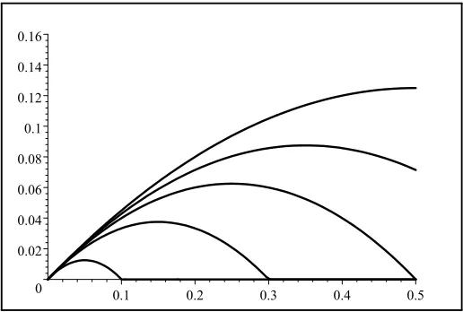
At that collusive price, the profit from the young isR(ˆp)/4 = 1/16 = 0.0625, while the profit from the young to an under-cutting firm is pmax{0,1−p/(1−β)}/2, see Figure 1 below. Note that the highest profit curve, corresponding toβ = 0, coincides with the deviation profit curve in the text-book model.
0 0.02 0.04 0.06 0.08 0.1 0.12 0.14 0.16
0.1 0.2 0.3 0.4 0.5
Figure 1: Deviation profit from the young, for β = 0, 0.3, 0.5, 0.7 and 0.9 (higher curves correspond to lowerβ).
Likewise, at the collusive price ˆp, the profit from the old is zero, while the profit from the old to an under-cuttingfirm in our model isp(1/2−p)/2, a parabola with maximum at p = 1/4 (this profit component being zero in the text-book model). Total profits to an under-cutting firm in our model thus is the sum of these two components - a continuous function for prices p < 1/2, with a kink at the price p= 1−β.
We study two extreme cases before tackling the general case.
condition (26) then boils down to
1−p∗ n ≥
¡
1−e−r/2¢p ∗
4. (27)
Since the candidate collusive prices are p∗ ∈ [0,1/2], it immediately follows that for n ≤ 4, all prices below the monopoly price are sustainable in subgame perfect equilibrium, for all discount factors r > 0. This is in contrast to the case ∆ = 1 in which all prices below the monopoly price are sustainable in subgame perfect equilibrium only under condition (3).
With more than four firms, the incentive condition (10) yields the following con-clusion: there is, for every collusive price p∗, a critical discount rate ¯r(p∗) such that p∗ is sustainable in subgame perfect equilibrium iff r ≤ r¯(p∗) (we presume here as elsewhere trigger strategies). It is straightforward to show that ¯r(p∗) decreases from infinity at p∗ = 4/(4 +n) to 2 ln [n/(n−4)] at p∗ = 1/2.
Maximally impatient consumers. When consumers are maximally impa-tient,β = 0, then the optimal deviation price is the solution of
max
p∈(0,p∗) p[p
∗−p+ max{0,1−p}], (28)
that is, p= (1 +p∗)/4 (see (26) and recall that p∗ ≤ 1/2). This implies that p∗ is sustainable in subgame perfect equilibrium iff
8 np
∗[1−p∗]≥¡1−e−r/2¢(1 +p∗)2. (29)
Rearranging terms we get
r≤2 ln
Ã
n(1 +p∗)2
n(1 +p∗)2−8p∗(1−p∗)
!
(30)
Intermediate Consumer Patience. Suppose consumer patience is in between the two above extremes. For anyβ ∈(0,1), the under-cutting price that maximizes the deviatingfirm’s profit is
ˆ
p= 1 +p ∗
2
1−β
2−β. (31)
(see (26)), so condition (26) becomes
1 np
∗[1−p∗]≥¡1−e−r/2¢1−β
2−β
µ
1 +p∗ 2
¶2
. (32)
In the special case when consumers have the same time preferences as the firms,
β =δ, and when the collusive price is the monopoly price, p∗ = 1/2, this condition boils down to
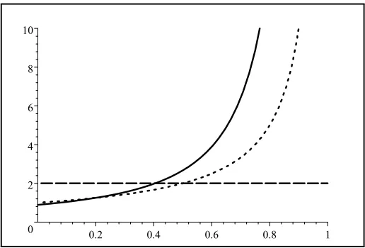
n≤ 4
9(2−δ) (1−δ) −2
. (33)
The graph of the function on the right hand side is illustrated in Figure 2 below, along with the graph for the corresponding function in the text-book model (dotted curve). We see that collusion is easier in the present model than in the text-book model, for any number n≥2 of firms in the market.
0 2 4 6 8 10
0.2 0.4 0.6 0.8 1
Figure 2: The largest number offirms, n, for which collusive monopoly pricing is possible, as a function of their discount factor β =δ in the present model (solid)
7.2. When the market period is shorter. We finally study all cases when ∆= 1/mfor any integer m≥2, but only in the special case when the collusive price is the monopoly price,p∗ = ˆp= 1/2. Then the equilibrium condition (21) becomes
1
4n(1−δ) ≥p∈max[0,1/2]H(p,p)ˆ (34)
whereδ =e−r/m is the firms’ discount factor, and
H(p,p) =ˆ
p³m+12 − m1−−ββp´ for p < 1−2β
p³32 − 21−−ββp´ for 1−2β ≤p≤1−β
p¡12 −p¢ for 1−β< p < 12
. (35)
In comparison with the general formula (22), this new formula distinguishes three, rather than two, price intervals. The reason is simply that the static demand function D in the present example vanishes at the price p = 1−β. Hence, at prices above that level, one of the terms in the right-hand side of (22) vanishes.
Figure 3 shows the graph of H(p, p∗) as a function of 0 < p < p∗ = 1/2, when β = 0.9, for m = 10 (solid curve) and m = 30 (dotted curve). The dashed curve is the corresponding graph in the text-book model, see (25). The diagram shows that the optimal deviation (for these parameter values) is not marginal under-cutting, as in the text-book model, but a significant price cut.
0 0.05 0.1 0.15 0.2 0.25 0.3
0.1 0.2 0.3 0.4 0.5
Figure 3: The deviation profit when β = 0.9, form = 10 (solid) and m= 30 (dotted).
is maximized at some price in the lowest of the three price intervals in (35). Moreover, the maximum deviation profit then is
V (r,∆) = max
p∈[0,1/2]H(p,p) =ˆ
1 16
(1 +∆)2¡1−e−r∆¢ ∆(1−∆e−r∆)
Hence, by (25), collusion at the monopoly price is easier to sustain than in the text-book model if and only if V (r,∆) < 1/4. Moreover, for any discount rate r > 0, V (r,∆) → r/16 as ∆ → 0. Thus, when the market period is very short, then collusion is easier to sustain in the present model than in the text-book model if and only if the common discount rate r for consumers and firms alike, is less than 4. (Recall thatr is the discount rate per time unit, where a time unit is the life-span of a consumer.)
8. Conclusion
Our model of dynamic Bertrand competition was developed in the simplest possible setting. In particular, we focused exclusively on the use of the “grim” trigger strategy as punishment. The reader might wonder to what extent our results are predicated on this restriction. We believe they are not. Consider, for example, the use of a forgiving trigger strategy with a finite punishment horizon. Firstly, just as in the text-book Bertrand model, a shorter price war as a punishment makes collusion less sustainable also in the present model. Secondly, the two forces, collusive and competitive, will again drive the results. It is easy to see that all our qualitative results are robust to this change of punishment strategies. Just as in the text-book Bertrand model, a shorter price war as punishment makes collusion less sustainable also in the present model. An investigation of the robustness of the present results with respect to punishment strategies more generally would be valuable.
Another simplification is that we have focused on the case of an indivisible durable good. It seems likely that the qualitative results carry over also to the case of divisible and non-durable goods - another task for future research.
A third avenue for further research is to investigate the effects of consumers’ intertemporal substitution possibilities on the sustainability of collusion in dynamic Cournot oligopoly.
References
[1] Ausubel L. and R. Deneckere (1987): “One is almost enough for monopoly”, Rand Journal of Economics 18, 255-274.
[3] Dutta, P. K. (1995): “A Folk theorem for stochastic games”, Journal of Eco-nomic Theory66, 1-32.
[4] Fudenberg, D. and J. Tirole (1991): Game Theory, MIT Press, Cambridge, MA.
[5] Gul F., H. Sonnenschein and R. Wilson (1986): “Foundations of dynamic monopoly and the Coase conjecture”, Journal of Economic Theory39, 155-190.
[6] Gul F. (1987): “Noncooperative collusion in durable goods oligopoly”, Rand Journal of Economics 18, 248-254.
[7] Maskin, E. and J. Tirole (1988): “A theory of dynamic oligopoly, II: Price competition, kinked demand curves andfixed costs”, Econometrica56, 571-600.
[8] Kirman A. and M. Sobel (1974): “Dynamic oligopoly with inventories”, Econo-metrica 42, 279-287.
[9] Radner, R. (1999): “Viscous demand”, mimeo., Stern School, NYU, New York.
[10] Selten R. (1965): “Spieltheoretische Behandlung eines Oligopolmodells mit Nachfragetr¨agheit”,Zeitschrift f¨ur die gesamte Staatswissenschaft121, 301-324, 667-689.
[11] Tirole J. (1988): The Theory of Industrial Organization, MIT Press, Cambridge, MA.