Volume 5, No. 8, Nov-Dec 2014
International Journal of Advanced Research in Computer Science
RESEARCH PAPER
Available Online at www.ijarcs.info
Gray Scale Image Denoising using PCA-SPT
Rajesh Kumar Sharma
Research Scholar, EC Department Oriental Institute of Science & TechnologyBhopal, India [email protected]
Abhishek Mishra
EC DepartmentOriental Institute of Science & Technology Bhopal, India
Mohd. Ahmed
HOD, EC DepartmentOriental Institute of Science & Technology Bhopal, India
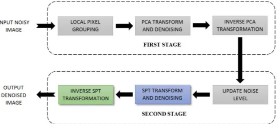
Abstract: This paper proposed a spatially adaptive image denoising scheme, which is comprised of two stages. In the first stage, image is denoised by using Principal Component Analysis (PCA) with Local Pixel Grouping (LPG). LPG-PCA can effectively preserve the image fine structures while denoising. In the second stage, we use Steerable Pyramid Transform (SPT) to decompose images into frequency sub-bands. The noise level is updated adaptively before second stage denoising. Steerable Pyramid Transform in the second stage further improves the denoising performance. This paper also reviews on the present denoising processes and performs their comparative study. Experimental results demonstrate that the proposed PCA-SPT algorithm achieve competitive outcomes. PCA-SPT works well in image fine structure preservation, compared with state-of-the-art denoising algorithms.
Keywords: AWGN; Wavelet; SPT; LPG-PCA; BM3D; Edge preservation.
I. INTRODUCTION
Digital image processing is a discipline that goes forward, to grow, with new application being developed at an invariably enhancing stride. It is a fascinating and stimulating field to be involved in today with application areas ranging from the entertainment industry to the space program. In the
21st century, a digital image is the best possible substitute to
convey visual information from one place to another. Digital image processing is a specific class of signal processing, whose primary objective is to extract the essential information from the contaminated images. Ideally, this is achieved with the help of computers, by applying some best available algorithms. As the essential information is extracted from the contaminated images the next step is to apply standard techniques to it, which will remove the artifacts presents in the contaminated image.
Image denoising shares an eminent portion of digital image processing, which is an essential step to remove the artifacts and improve the tone of the images. It is a prerequisite for many image processing tasks like image classification, image registration, image restoration, image segmentation and object recognition, where it is essential to suppress the artifacts from the noisy image to get the approximately original image. Noise will be brought into an image through the image acquisition process such as quantization, transmission due to a noisy channel and errors from the measurement process. Each step of the image acquisition process successively degrades image such as lenses, film, digitizer, etc. contribute to the degradation procedure.
Image denoising is an obligatory procedure in real world applications such as photography where an image was necessarily degraded but needs to be improved before it can be published. For this type of application, we have to develop a model [1], which better describes the degradation process.
This model helps to determine the inverse process, which can be applied to the image to get it back into the original form. Space exploration is one such example in which image restoration is frequently used to eradicate artifacts, generated by mechanical movement of the space vehicle or to reduce distortion in the optical system of a telescope. Astronomy is another important application, where we generally deal with the images of poor resolution. Image processing plays an important role in the medical science imaging system also, where quality processing techniques are required for probing images of unparalleled events and in forensic science, to enhance the quality of potentially useful photographic evidence of extremely bad quality.
Usually noise will be necessarily introduced in the image acquisition process. Hence it is necessary to remove noise by any means before using it in any application, to improve the quality of image. From the earlier smoothing filters and frequency domain denoising methods [2] to the lately developed wavelet [3,4,5,6,7,8,9,10,11,12], curvelet [13] and ridgelet [14] based methods, adaptive principle component analysis [15], bilateral filtering [16,17], non-local mean based methods [18,19], sparse representation [20] and K-SVD [21] methods, shape-adaptive transform [22], non-local collaborative filtering [23] and local pixel grouping with principle component analysis [24] and more, are some of the many directions and tools explored in studying this problem. With the rapid development of modern digital imaging devices and their increasingly wide applications in our daily life, there are increasing requirements of new denoising algorithms for higher image quality.
accomplished by transforming back the processed wavelet coefficients into spatial domain. Late development of WT denoising includes ridgelet and curvelet methods for line structure preservation. Although WT has demonstrated its efficiency in denoising, it uses a fixed wavelet basis to represent the image. For natural images, however, there is a rich amount of different local structural patterns, which cannot be well represented by using only one fixed wavelet basis. Therefore, WT-based methods can introduce many visual artifacts in the denoising output.
To overcome the problem of WT, in [15] Muresan and Parks proposed a spatially adaptive principal component analysis (PCA) based denoising scheme, which computes the locally fitted basis to transform the image. Elad and Aharon [20,21]proposed sparse redundant representation and K-SVD based denoising algorithm by training a highly over-complete dictionary. Foi et al. [22] applied a shape-adaptive discrete cosine transform (DCT) to the neighborhood, which can achieve very sparse representation of the image and hence lead to effective denoising. All these methods show better denoising performance than the conventional WT-based denoising algorithms.
Recently established non-local means (NLM) approaches [26]use a very different viewpoint from the above methods, where the similar image pixels are averaged according to their intensity distance. In [18], the NLM denoising background was well established. Each pixel is estimated as the weighted average of all the pixels in the image, and the weights are determined by the similarity between the pixels. This structure was enhanced in [19], where the pair wise hypothesis testing was used in the NLM estimation. Inspired by the achievement of NLM methods, recently Dabov et al. [23], proposed a collaborative image denoising scheme by patch matching and sparse 3D transform. They searched for similar blocks in the image by using block matching and grouped those blocks into a 3D cube. A sparse 3D transform was then applied to the cube and noise was suppressed by applying Wiener filtering in the transformed domain. The so-called BM3D scheme accomplishes amazing denoising results yet its implementation is a little multifarious.
Recently a novel denoising scheme named LPG-PCA [24] is developed which can effectively preserve the image fine structures while smoothing noise. By transforming the original dataset into PCA domain and preserving only the several most significant principal components, the noise can be removed. In [15], a PCA-based scheme was suggested for image denoising by using a moving window to calculate the local statistics, from which the local PCA transformation matrix was estimated.
In this paper we present an efficient LPG-PCA based denoising method with steerable pyramid transform (SPT). In the proposed PCA-SPT scheme, we model a pixel and its adjacent pixels as a vector variable. The training samples of
this variable are selected by block matching scheme. With this LPG technique, the local statistics of the variables can be accurately calculated so that the image edge structures can be well preserved after shrinkage in the PCA domain for noise removal. As shown in Figure 1, the proposed PCA-SPT algorithm has two stages. The first stage yields an initial estimation of the image by removing most of the noise content and the second stage will further refine the output of the first stage.
The first stage use the equivalent procedures as done in LPG-PCA denoising scheme, but in the second stage we use Steerable Pyramid Transform, to decompose images into frequency sub-bands. Before applying the second stage the level of noise is updated adaptively. The transform is implemented in the Fourier domain [10], allowing exact reconstruction of the image from the sub-bands. Since the noise is significantly reduced in the first stage, we do not use LPG in the second stage, which intern reduces the computational cost of the entire scheme. Compared with the BM3D algorithm, the proposed PCA-SPT technique can use a relatively small local window, like LPG-PCA algorithm to group the similar pixels for PCA training with reduced computational cost, yet it yields competitive results with state-of-the-art BM3D algorithm.
II. FIRST STAGE DENOISING PROCEDURE
It is clear that, denoising is a process to estimate and remove noise, from the corrupted images, Hence to create a denoising model, it is necessary to know about the noise type which contaminates the image. Here we assume that the noise which contaminates the original image is Additive
White Gaussian Noise with zero mean and standard
deviation , i.e. , where is the noisy image.
The original image and noise are presumed to be
uncorrelated. The objective of denoising model is to find
estimation, denoted by of from the observation . The
denoised image is anticipated to be as close to as possible. The spatial location and intensity are the two parameters through which an image pixel may be described, while the local structure of the image represented as a set of neighboring pixels at different intensity levels. Since most of the important information of an image is expressed by its edge structures, hence edge preservation is most important in image denoising. To achieve the previously specified goal, in this paper we model a pixel and its nearest neighbors as a vector variable and execute noise reduction on the vector instead of the single pixel.
To model a vector variable we create a window
centered on the fundamental pixel to be denoised. It is
denoted by , the vector
[image:2.595.168.446.646.770.2]containing all the elements within the window.
Since the image considered here is noisy, hence it is denoted by
The noisy vector of , where ,
and , to calculate
from , we consider them as noiseless and noisy vector
variables respectively, so that the statistical methods such as PCA may be used.
In order to eliminate the noise from by using PCA
transform, a set of training samples of is required so that
PCA transformation matrix can be calculated in terms of
covariance matrix of . To find the training samples, we
create a training block of size centered on ,
as demonstrated in Figure 2. It is very easy to take the image
pixel in each possible block of size within the training
[image:3.595.330.555.64.290.2]block of size as the samples of noisy variable .
Figure 2. Illustration of the modeling of first stage denoising
In this way, there are totally training
samples for each component of . However, there may be
very different blocks from the given central block in
the training window so that taking all the
blocks as the training samples of will lead to wrong
approximation of the covariance matrix of . Inaccurate
approximation of the PCA transformation matrix will occur due to faulty estimate of the training samples, which intern increases the noise residuals in the denoised image. Hence, it is very essential to select and group the training samples before employing the PCA for denoising, which is similar to
the central block.
Grouping of the training samples is same as to the central
block in the training window. It is surely a
classification scheme that may be realized by various techniques such as block matching, correlation-based matching, fuzzy clustering [27], K-means clustering [28], self-organizing maps [29] etc. and choice of this algorithm is based on different criteria. Among them, the block matching method is very simple and efficient. Hence we use block matching method for local pixel grouping procedure.
There are totally possible training blocks of
in the training window. We used the fact that noise
is AWGN and uncorrelated with signal. For computing the PCA transformation matrix it is necessary, that there should be adequate number of samples. To estimate the image local statistics optimized training samples are used. They are robust and make the algorithm more stable to estimate the PCA transformation matrix. The next step is how to calculate
the noiseless dataset from the noisy observation . Once
we get the central block and the central pixel under test
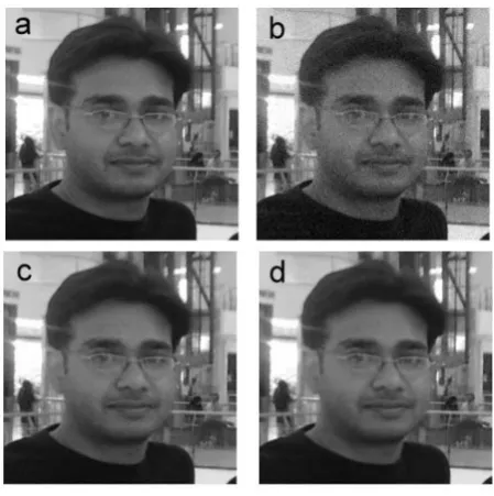
Figure 3. (a) Original image Rajesh; (b) noisy image (PSNR= 28.1 dB);
(c) denoised image after the first stage of the proposed method (PSNR= 35.5 dB) and (d) denoised image after the second stage of the proposed method (PSNR=36.2 dB). We see that the visual quality is much improved after the second stage refinement.
can be extracted. Now each pixel is processed by such scheme, to denoise the entire image .
III. SECOND STAGE DENOISING PROCEDURE
As discussed in the above section, LPG-PCA procedure will remove most of the noise present in the image under test. Still, the denoised image has as much noise residual, which makes the image visually unpleasant. Figure 3 shows an example of image Rajesh. Figure 3(a) is the original image
Rajesh; Figure 3(b) is the noisy version of it ( ,
PSNR=28.1dB, SSIM=0.6355); Figure 3(c) is the denoised image (PSNR= 35.5 dB, SSIM= 0.9243) by using the basic LPG-PCA scheme. Although both the parameters PSNR and SSIM are much improved, still we can see much noise residual in the output denoising image. One of the basic reasons for the presence of noise residual in the denoised
image is that the original dataset is
contaminatedwithstrong noise, which makes the covariance
matrix noisier and leads to estimation bias of the PCA
transformation matrix. This in turn degrades the performance of denoising procedure.
Original dataset contaminated with strong noise is another reason that leads to LPG errors, which accordingly leads to the estimation bias of the covariance matrix
(or ). Thus, for a better noise reduction, it is necessary
to remove noise residuals present after denoising. Since, most of the noise is removed by first stage LPG-PCA denoising procedure, which can improve the accuracy and
the estimation of (or ) of the denoised image. Now
[image:3.595.51.283.263.402.2]decomposes images into frequency sub-bands, here the noise residuals present after second stage is easily suppressed.
Noise level should be updated before the second stage of proposed denoising method. Here we consider noisy image as and is the denoised image after first denoising stage.
Denoised image can be expressed as , where is
the noise residual in the first stage denoised image. To initialize the second denoising stage, it is important to
estimation the level of , which is denoted by .
Now input it to the second stage of proposed denoising
method. Noise level is estimated based on the difference
between and . This is expressed by
We have:
Noise residual is assumed as the low noise variant of
noise , and it has only the low frequency portion of .Let is the difference between them and has only
the high frequency portion of . There is
. Generally, is very small as
compared with . For the convenience of development,
we remove from , and let
Thus from we have
In practice will include not only the noise residual but
also the estimation error of noiseless image . Therefore, in implementation we assume that
where is a constant. The value of is estimated
experimentally and around 0.35 gives satisfying results
for all the test images used in this experiment.
For second stage of denoising, we use a transform known as a steerable pyramid [30,31] to decompose images into frequency sub-bands. The procedure for second stage denoising uses the structure as: 1) decompose the image in sub-bands by pyramid transform at diverse scales and orientations; 2) estimate and remove noise from each sub-band, except for the low pass residual band; and 3) estimate inverse pyramid transform, obtaining the denoised image. We assume the image is contaminated only by noise residuals remains after the first stage denoising. A vector corresponding to a neighborhood of observed coefficients of the pyramid representation can be expressed as
where random vector is a Gaussian scale mixture if and only if it can be expressed as the product of a zero-mean
Gaussian vector and an independent positive scalar
random variable as
Both and are zero-mean Gaussian vectors, with
associated covariance matrices and . The density of
the detected neighborhood vector trained on is a zero-mean Gaussian, with covariance
The covariance of neighborhood noise, is accomplished
by dividing a delta function into pyramid
sub-bands, where are the image dimensions. This
signal has the same power spectrum as the noise, but it is
free from random fluctuations. Elements of may then
are computed directly as sample covariance (i.e., by averaging the products of pairs of coefficients over all the neighborhoods of the sub-band). This technique is certainly comprehensive for nonwhite noise, by swapping the delta function with the inverse Fourier transform of the square root of the noise power spectral density. Note that the entire procedure may be performed off-line, as it is signal
independent. Given , the signal covariance can
becomputed from the observation covariance matrix .We
compute from by taking expectations over :
Without loss of generality, we set , resulting in:
We force to be positive semi definite by performing
Eigen vector decomposition and setting any possible negative Eigen values (nonexistent or negligible, in most cases) to zero. Figure 3(d) shows the denoising results (PSNR=36.2 dB) of Image Rajesh after the second denoising stage. Although the PSNR is improved by only 0.7 dB, but the visual quality of the image is much improved by effectively removing the noise residual in the second denoising stage.
IV. EXPERIMENTAL RESULT AND ANALYSIS
The concept of the proposed PCA-SPT algorithm is carried from the antecedently developed LPG-PCA denoising algorithm. The proposed PCA-SPT algorithm is a prolongation of the LPG-PCA denoising algorithm [24].We used 8 different images to enumerate the performance of the proposed algorithm. Our dataset includes standard test images and one image of the author. We will evaluate the data for Barbara, Boat, Cameraman, House, Lena, Monarch, Peppers and Rajesh shown in Figure 4. All of our images are
8-bit gray scale images of dimension and are
converted to same image format (i.e. TIF) using MATLAB. The results presented in this paper are obtained by adding simulated AWGN to true noiseless images. After denoising the results are compared with the true noiseless image for performance evaluation. Due to the space limitation, we demonstrate the comparison result of proposed scheme with only some values of noise level. We analyzed the complete
dataset of test images with noise levels
i.e. .
To represent the denoising performance of our algorithm, we compare the proposed scheme with four representative and state-of-the-art denoising algorithms: the wavelet-based denoising methods [3,6]; Po-Edges denoising methods[10]; LPG-PCA denoising method [24] and the recently developed BM3D denoising method[23]. The BM3D algorithm is state-of-the-art denoising algorithm and it has been considered as a standard for developing novel denoising algorithm.
Figure 4. The test images Barbara, Boat, Cameraman, House, Lena, Monarch, Peppers, and Rajesh
Table I. The PSNR (dB) and SSIM results of the denoised images in the two stages by the proposed PCA-SPT method.
Image Barbara Boat Cameraman House
Stage - I
34.1 (0.9314) 33.0 (0.9086) 33.5 (0.9026) 35.6 (0.8954)
30.0 (0.8387) 28.8 (0.7888) 29.3 (0.7704) 31.6 (0.7750)
27.4 (0.7396) 26.6 (0.6817) 27.0 (0.6481) 28.9 (0.6535)
25.6 (0.6519) 24.9 (0.5882) 25.2 (0.5406) 26.9 (0.5487)
Stage - II
34.5 (0.9418) 33.2 (0.9191) 33.7 (0.9252) 36.2 (0.9134)
30.7 (0.8821) 29.3 (0.8331) 30.0 (0.8654) 33.1 (0.8643)
28.5 (0.8244) 27.4 (0.7717) 28.0 (0.8124) 31.1 (0.8331)
27.0 (0.7809) 26.0 (0.7196) 26.6 (0.7751) 29.8 (0.8063)
Image Lena Monarch Peppers Rajesh
Stage - I
34.0 (0.9174) 33.7 (0.9397) 33.9 (0.9089) 35.5 (0.9243)
29.9 (0.8180) 29.5 (0.8531) 30.0 (0.8123) 31.1 (0.8133)
27.5 (0.7146) 26.9 (0.7586) 27.5 (0.7041) 28.5 (0.7004)
25.7 (0.6210) 25.2 (0.6766) 25.6 (0.6057) 26.5 (0.5978)
Stage - II
34.4 (0.9308) 33.9 (0.9538) 34.2 (0.9217) 36.2 (0.9464)
30.7 (0.8776) 30.2 (0.9129) 30.7 (0.8745) 32.4 (0.9020)
28.6 (0.8303) 27.8 (0.8692) 28.6 (0.8292) 30.4 (0.8633)
27.2 (0.7911) 26.4 (0.8336) 27.1 (0.7929) 28.7 (0.8295)
The value in the parenthesis is the SSIM measure
required which contain a family of related M-files and possibly MEX-files.
PSNR and SSIM [32] values of the first stage and second stage of the proposed scheme on the set of test images are enlisted in Table I and Second stage of the proposed method verify that the improvement of the PSNR values. On the observation of the result, we ensure that the second stage of the proposed algorithm can improve the values of PSNR from 0.2–2.9 dB. For different images under different noise level ( is from 10 to 40). Sometimes values of PSNR measure will not improve so much in the second stage, thus another parameter called SSIM[32] is used to represent the image visual quality. For instance, image Monarch, with
noise level , the SSIM measure is much increased
from 0.7586 to 0.8692 after the second stage refinement, while the PSNR is raised by only 0.9 dB.
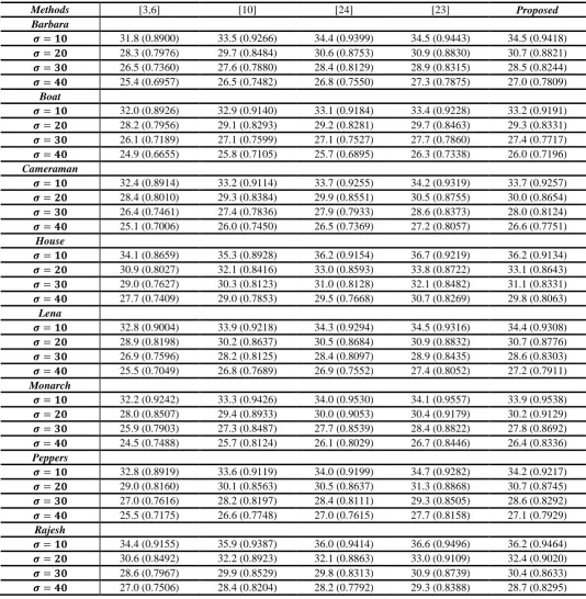
PSNR and SSIM measures of previously established denoising scheme and the proposed method on the 8 test images are summarized in Table II. Let’s first see the PSNR measures by different methods. From Table II we observe that the BM3D filtering method of denoising has the highest PSNR measures. The PSNR result of proposed method is higher than the wavelet [3,6], Po-Edges [10], LPG-PCA [24]and the wavelet-based method [3,6] has the lowest PSNR value. Let’s then focus on the SSIM measure and the visual quality evaluation of these denoising algorithms. From Table II it is clear, that BM3D has the highest SSIM measures. The proposed PCA-SPT has higher SSIM measures than LPG-PCA [24]. Again, the wavelet-based denoising methods have the lowest SSIM measures.
[image:5.595.35.566.290.584.2]the denoising results of the two test images with noise
level by different methods. The subfigure (a) is the
original image; subfigures (b–f) are the denoised images by the scheme in [3,6], [10], [24], [23]and the proposed PCA-SPT method respectively. We see that although BM3D has higher SSIM measures than proposed PCA-SPT method, their denoised images are analogous in real visual observation, and they have much improved visual quality than all the other techniques. Graphical representation of PSNR and SSIM measures for image Monarch by different schemes are shown in Figures 6-7and for image Peppers in Figures 9-10 respectively.
[image:6.595.30.565.210.756.2]The graph shows that when the PSNR measure of the proposed scheme is almost equals to the other methods the SSIM measure has a great variance even for the high noise level. The LPG-PCA scheme generates many artifacts in the denoised image. The wavelet based denoising methods [3,6]have the worst visual quality. This is because in WT, the fixed wavelet basis function is used to de-correlate the many different image structures. Often this is not efficient enough to represent the image content so that many denoising errors appear.
Table II. The PSNR (dB) and SSIM results of the denoised images at different noise levels and by different schemes.
Methods [3,6] [10] [24] [23] Proposed
Barbara
31.8 (0.8900) 33.5 (0.9266) 34.4 (0.9399) 34.5 (0.9443) 34.5 (0.9418)
28.3 (0.7976) 29.7 (0.8484) 30.6 (0.8753) 30.9 (0.8830) 30.7 (0.8821)
26.5 (0.7360) 27.6 (0.7880) 28.4 (0.8129) 28.9 (0.8315) 28.5 (0.8244)
25.4 (0.6957) 26.5 (0.7482) 26.8 (0.7550) 27.3 (0.7875) 27.0 (0.7809)
Boat
32.0 (0.8926) 32.9 (0.9140) 33.1 (0.9184) 33.4 (0.9228) 33.2 (0.9191)
28.2 (0.7956) 29.1 (0.8293) 29.2 (0.8281) 29.7 (0.8463) 29.3 (0.8331)
26.1 (0.7189) 27.1 (0.7599) 27.1 (0.7527) 27.7 (0.7860) 27.4 (0.7717)
24.9 (0.6655) 25.8 (0.7105) 25.7 (0.6895) 26.3 (0.7338) 26.0 (0.7196)
Cameraman
32.4 (0.8914) 33.2 (0.9114) 33.7 (0.9255) 34.2 (0.9319) 33.7 (0.9257)
28.4 (0.8010) 29.3 (0.8384) 29.9 (0.8551) 30.5 (0.8755) 30.0 (0.8654)
26.4 (0.7461) 27.4 (0.7836) 27.9 (0.7933) 28.6 (0.8373) 28.0 (0.8124)
25.1 (0.7006) 26.0 (0.7450) 26.5 (0.7369) 27.2 (0.8057) 26.6 (0.7751)
House
34.1 (0.8659) 35.3 (0.8928) 36.2 (0.9154) 36.7 (0.9219) 36.2 (0.9134)
30.9 (0.8027) 32.1 (0.8416) 33.0 (0.8593) 33.8 (0.8722) 33.1 (0.8643)
29.0 (0.7627) 30.3 (0.8123) 31.0 (0.8128) 32.1 (0.8482) 31.1 (0.8331)
27.7 (0.7409) 29.0 (0.7853) 29.5 (0.7668) 30.7 (0.8269) 29.8 (0.8063)
Lena
32.8 (0.9004) 33.9 (0.9218) 34.3 (0.9294) 34.5 (0.9316) 34.4 (0.9308)
28.9 (0.8198) 30.2 (0.8637) 30.5 (0.8684) 30.9 (0.8832) 30.7 (0.8776)
26.9 (0.7596) 28.2 (0.8125) 28.4 (0.8097) 28.9 (0.8435) 28.6 (0.8303)
25.5 (0.7049) 26.8 (0.7689) 26.9 (0.7552) 27.4 (0.8052) 27.2 (0.7911)
Monarch
32.2 (0.9242) 33.3 (0.9426) 34.0 (0.9530) 34.1 (0.9557) 33.9 (0.9538)
28.0 (0.8507) 29.4 (0.8933) 30.0 (0.9053) 30.4 (0.9179) 30.2 (0.9129)
25.9 (0.7903) 27.3 (0.8487) 27.7 (0.8539) 28.4 (0.8822) 27.8 (0.8692)
24.5 (0.7488) 25.7 (0.8124) 26.1 (0.8029) 26.7 (0.8446) 26.4 (0.8336)
Peppers
32.8 (0.8919) 33.6 (0.9119) 34.0 (0.9199) 34.7 (0.9282) 34.2 (0.9217)
29.0 (0.8160) 30.1 (0.8563) 30.5 (0.8637) 31.3 (0.8868) 30.7 (0.8745)
27.0 (0.7616) 28.2 (0.8197) 28.4 (0.8111) 29.3 (0.8505) 28.6 (0.8292)
25.5 (0.7175) 26.6 (0.7748) 27.0 (0.7615) 27.7 (0.8158) 27.1 (0.7929)
Rajesh
34.4 (0.9155) 35.9 (0.9387) 36.0 (0.9414) 36.6 (0.9496) 36.2 (0.9464)
30.6 (0.8492) 32.2 (0.8923) 32.1 (0.8863) 33.0 (0.9109) 32.4 (0.9020)
28.6 (0.7967) 29.9 (0.8529) 29.8 (0.8313) 30.9 (0.8739) 30.4 (0.8633)
27.0 (0.7506) 28.4 (0.8204) 28.2 (0.7792) 29.3 (0.8388) 28.7 (0.8295)
Figure 5. The denoising results of Monarch by different schemes. (a) Noiseless Monarch; denoised images by methods (b)[3,6]; (c) [10]; (d) [24]; (e) [23]; and (f) the proposed PCA-SPT method.
Figure 6. Graphical representation of PSNR measure (in dB) for
imageMonarch by different schemes.
Figure 7. Graphical representation of SSIM measure for imageMonarch by
[image:7.595.35.285.269.465.2]different schemes.
Figure 8. The denoising results of Peppers by different schemes. (a)
[image:7.595.307.553.272.466.2]Noiseless Monarch; denoised images by methods (b)[3,6]; (c) [10]; (d) [24]; (e) [23]; and (f) the proposed PCA-SPT method.
Figure 9. Graphical representation of PSNR measure (in dB) for image
Peppers by different schemes.
Figure 10. Graphical representation of SSIM measure for image Peppers by
different schemes. 32.2 28.0 25.9 24.5 33.3 29.4 27.3 25.7 34.0 30.0 27.7 26.1 34.1 30.4 28.4 26.7 33.9 3 0 .2 27.8 26.4 24.0 26.0 28.0 30.0 32.0 34.0 36.0
10 20 30 40
P SNR i n d b SIGMA PSNR MONARCH
WAVELET Po-Edges LPG-PCA BM3D Proposed
0.92 42 0.850 7 0.790 3 0.74 88 0.94 26 0.89 33 0.84 87 0.81 24 0.95 3 0.90 53 0.85 39 0.80 29 0.95 57 0.91 79 0.88 22 0.84 46 0.95 38 0 .9 1 2 9 0.869 2 0.83 36 0.7 0.75 0.8 0.85 0.9 0.95 1
10 20 30 40
SS
IM
SIGMA
SSIM MONARCH
WAVELET Po-Edges LPG-PCA BM3D Proposed
32.8 29.0 27.0 25.5 33.6 30.1 28.2 26.6 34.0 30.5 28.4 27.0 34.7 31.3 29.3 27.7 34.2 30.7 28.6 27.1 24.0 26.0 28.0 30.0 32.0 34.0 36.0
10 20 30 40
P SNR i n d b SIGMA PSNR PEPPERS
WAVELET Po-Edges LPG-PCA BM3D Proposed
0.89 19 0.81 6 0.76 16 0.71 75 0.91 19 0.85 63 0.81 97 0.77 48 0.91 99 0.863 7 0.81 11 0.76 15 0.92 82 0 .8 8 6 8 0.85 05 0.81 58 0.92 17 0.87 45 0.82 92 0.79 29 0.7 0.75 0.8 0.85 0.9 0.95 1
10 20 30 40
SS
IM
SIGMA
SSIM PEPPERS
[image:7.595.307.554.510.704.2] [image:7.595.34.285.512.704.2]The proposed PCA-SPT denoising procedure uses PCA to adaptively compute the local image decomposition transform so that it can better represent the image local structure. In addition, the SPT operation is employed to eliminate the noise residuals present after first stage denoising, that decompose images into frequency sub-bands. Before applying the second stage the level of noise is update adaptively. The transform is implemented in the Fourier domain, allowing exact reconstruction of the image from the sub-bands. The denoised images by BM3D and the proposed scheme are very comparable in terms of visual quality. Both of them can well preserve the image edges and remove the noise without introducing too many artifacts. Although the PSNR and SSIM measure of PCA-SPT are lower than that of BM3D, PCA-SPT has competitive results in the preservation of small edge structure as the original LPG-PCA method.
BM3D works better in preserving large-grain edges and denoising smoothing areas (e.g. the image Peppers), where there are a rich amount of non-local redundancies that could be exploited, while PCA-SPT works well in preserving small-grain edges (e.g. the image Monarch), where BM3D may generate some artifacts because there are not so many non-local redundancies around those structures.
In summary, as a non-local collaborative denoising scheme, BM3D can successfully exploit the non-local redundancy in the image to suppress noise. Therefore, it could have very high PSNR and SSIM measures. However, for fine-grain structures, improper non-local information may be introduced by BM3D for image restoration so that errors may be produced in those areas. Although the LPG-PCA scheme works well for fine-grain preservation but its computational cost is high than PCA-SPT since it uses block matching in both stages. The computational cost of PCA-SPT is very low than LPG-PCA algorithm, hence PCA-SPT works well in small structure preservation with low computational cost.
V. CONCLUSION
The proposed PCA-SPT denoising method employs PCA transform with LPG in first stage. Principal component analysis adaptively calculate the vector decomposition of the target image, hence it can better represent the local structure of image and local pixel grouping, which ensure that only the right samples of pixels are needed in the training of PCA transform. In addition to PCA with LPG operation we incorporate the second stage, in which SPT is used. Computational cost of the second stage is approximately one fourth of the first stage of LPG-PCA algorithm. Thus the overall cost of the proposed algorithm is very low and we get the denoising result in less time than that required in LPG-PCA algorithm. It provides a good compromise between the accuracy and the execution time: it is much faster and considerably more accurate than the LPG-PCA algorithm.
VI. REFERENCES
[1] Scott E. Umbaugh, Digital image processing and
analysis: human and computer vision applications with CVIPtools.: CRC press, 2010.
[2] Rafael C. Gonzalez, Richard E. Woods, and Steven L.
Eddins, Digital Image Processing , 2nd ed. Englewood
Cliffs, NJ: Prentice- Hall, 2002.
[3] D. L. Donoho, "Denoising by soft thresholding," IEEE
Transactions on Information Theory, pp. 613–627, 1995.
[4] R. R. Coifman and D. L. Donoho, Translation-invariant
de-noising, G. Oppenheim, Ed. Berlin, Germany: Springer, 1995.
[5] M. K. Mıhcak, I. Kozintsev, K. Ramchandran, and Moulin P., "Low-complexity image denoising based on
statistical modeling of wavelet coefficient," IEEE Signal
Processing Letters, vol. VI, no. 12, pp. 300–303, 1999.
[6] S. G. Chang, B. Yu, and M. Vetterli, "Spatially adaptive wavelet thresholding with context modeling for image denoising," IEEE Transaction on Image Processing, vol. IX, no. 9, pp. 1522–1531, 2000.
[7] A. Pizurica, W. Philips, I. Lamachieu, and M. Acheroy, "A joint inter- and intrascale statistical model for
Bayesian wavelet based image denoising," IEEE
Transaction on Image Processing , vol. V, no. 11, pp.
545–557, 2002.
[8] L Zhang, B Paul, and X Wu, "Hybrid inter- and intra
wavelet scale image restoration," Pattern Recognition,
vol. VIII, no. 36, pp. 1737–1746, 2003.
[9] Z Hou, "Adaptive singular value decomposition in
wavelet domain for image denoising," Pattern
Recognition, vol. VIII, no. 36, pp. 1747–1763, 2003.
[10] J. Portilla, V. Strela, M. J. Wainwright, and E. P. Simoncelli, "Image denoising using scale mixtures of
Gaussians in thewavelet domain," IEEE Transaction on
Image Processing , vol. XI, no. 12, pp. 1338–1351, 2003. [11] P. Bao, X. Wu L. Zhang, "Multiscale LMMSE-based
image denoising with optimalwavelet selection," IEEE
Transaction on Circuits and Systems for Video Technology, vol. IV, no. 15, pp. 469–481, 2005.
[12] A. Pizurica and W. Philips, "Estimating the probability of the presence of a signal of interest in multiresolution
single and multiband image denoising," IEEE
Transaction on Image Processing, vol. III, no. 15, pp. 654–665, 2006.
[13] J. L. Starck, E. J. Candes, and D. L. Donoho, "The
curvelet transform for image denoising," IEEE
Transaction on Image Processing, vol. VI, no. 11, pp. 670–684, 2002.
[14] G. Y. Chen and B. Kegl, "Image denoising with complex
ridgelets," Pattern Recognition, vol. II, no. 20, pp. 578–
585, 2007.
[15] D. D. Muresan and T. W. Parks, "Adaptive principal components and image denoising," in Proceedings of the 2003 International Conference on Image Processing, vol. 1, 14–17 September 2003, pp. 101–104.
[16] C. Tomasi and R. Manduchi, "Bilateral filtering for gray and colour images," in IEEE International Conference on Computer Vision, Bombay, India, 1998, pp. 839–846.
[17] D. Barash, "A fundamental relationship between bilateral filtering, adaptive smoothing, and the nonlinear diffusion
equation," IEEE Transaction on Pattern Analysis and
Machine Intelligence, vol. VI, no. 24, pp. 844–847, 2002.
[18] A. Buades, B. Coll, and J. M. Morel, "A review of image
denoising algorithms, with a new one," Multiscale
Modeling Simulation, vol. II, no. 4, pp. 490–530, 2005.
[19] C. Kervrann and J. Boulanger, "Optimal spatial
adaptation for patch based image denoising," IEEE
[20] M. Elad and M. Aharon, "Image denoising via sparse and redundant representations over learned dictionaries," IEEE Transaction on Image Processing, vol. XII, no. 15, pp. 3736–3745, 2006.
[21] M Aharon, M Elad, and A M Bruckstein, "The K-SVD: an algorithm for designing of overcomplete dictionaries
for sparse representation," IEEE Transaction on Signal
Processing, vol. XI, no. 54, pp. 4311–4322, 2006.
[22] A. Foi, V. Katkovnik, and K. Egiazarian, "Pointwise shape-adaptive DCT for high quality denoising and
deblocking of grayscale and color images," IEEE
Transaction on Image Processing, vol. V, no. 16, 2007.
[23] K. Dabov, A. Foi, V. Katkovnik, and Egiazarian K., "Image denoising by sparse 3D transform-domain
collaborative filtering," IEEE Transaction on Image
Processing, vol. VIII, no. 16, pp. 2080–2095, 2007.
[24] L. Zhang, W. Dong, D. Zhang, and G. Shi, "Two-stage image denoising by principal component analysis with
local pixel grouping," Pattern Recognition, vol. IV, no.
43, pp. 1531-1549, 2010.
[25] S. Mallat, A Wavelet Tour of Signal Processing. New
York: Academic Press, 1998.
[26] L. P. Yaroslavsky, Digital Signal Processing—An
Introduction. Berlin: Springer, 1985.
[27] F. Höppner, F. Klawonn, R. Kruse, and t Runkler, Fuzzy
Cluster Analysis. Chichester: Wiley, 1999.
[28] J. B. MacQueen, "Some methods for classification and
analysis of multivariate observations," in Berkeley
Symposium on Mathematical Statistics and Probability, Berkeley, 1967, pp. 281–297.
[29] T. Kohonen, Self-Organizing Maps, 2nd ed. Heidelberg:
Information Sciences Springer, 1997.
[30] E. P. Simoncelli, W. T. Freeman, E. H. Adelson, and D. J.
Heeger, "Shiftable multi-scale transforms," IEEE
Transaction on Information Theory, vol. 38, pp. 587–607, Mar 1992.
[31] W. T. Freeman and E. H. Adelson, "The design and use
of steerable filters," IEEE Pattern Anal. Machine Intell.,
vol. 13, no. 9, pp. 891–906, 1991.
[32] Z. Wang, A.C. Bovik, H.R. Sheikh, and E.P. Simoncelli, "Image quality assessment: from error visibility to
structural similarity," IEEE Transaction on Image

![Figure 8. The denoising results of Peppers by different schemes. (a) Noiseless Monarch; denoised images by methods (b)[3,6]; (c) [10]; (d) [24]; (e) [23]; and (f) the proposed PCA-SPT method](https://thumb-us.123doks.com/thumbv2/123dok_us/695132.1077158/7.595.307.554.510.704/figure-denoising-peppers-different-noiseless-monarch-denoised-proposed.webp)
