Lists in a Lighthouse

(1)

University of South Carolina

Scholar Commons

Theses and Dissertations

5-8-2015

Diagnostics and Model Selection for Generalized

Linear Models and Generalized Estimating

Equations

Chelsea Boquet Deroche University of South Carolina - Columbia

Follow this and additional works at:https://scholarcommons.sc.edu/etd

Part of theEpidemiology Commons

This Open Access Dissertation is brought to you by Scholar Commons. It has been accepted for inclusion in Theses and Dissertations by an authorized administrator of Scholar Commons. For more information, please [email protected].

Recommended Citation

(2)

DIAGNOSTICS AND MODEL SELECTION FOR GENERALIZED

LINEAR MODELS AND GENERALIZED ESTIMATING EQUATIONS

by

Chelsea Boquet Deroche

Bachelor of Science Nicholls State University, 2009

Master of Science

Louisiana State University, 2011

Submitted in Partial Fulfillment of the Requirements

For the Degree of Doctor of Philosophy in

Biostatistics

The Norman J. Arnold School of Public Health

University of South Carolina

2015

Accepted by:

James W. Hardin, Major Professor

Suzanne McDermott, Committee Member

Bo Cai, Committee Member

Kevin Bennett, Committee Member

(3)

(4)

DEDICATION

I dedicate this dissertation to my loving and understanding husband Joshua

Deroche, my encouraging and compassionate parents Kevin and Martina (Tina) Boquet

and sister Lindsey, and my supportive and forever proud grandparents William (Bill) and

Katherine (Kat) Smith. Your unlimited support, encouragement, constant love and

patience has sustained me throughout this process. I appreciate everything you have done

for me, and I am blessed to have you all in my life. I love you all more than you all will

(5)

ACKNOWLEDGEMENTS

I would like to thank my major advisor, Dr. James W. Hardin for agreeing to

mentor me and challenging me in the process. You have been extremely supportive, very

patient, and encouraging throughout the entire dissertation process. Thank you for being

there for the many weekly meetings, long coding sessions, manuscript and dissertation

edits, and random life advice. You mentorship has strengthened my statistical writing

skills and statistical consulting ability. Thank you for taking the time to sit down with me

and teach me to code in Stata. Without your creative suggestions, I would not have been

able to discover so many areas of research in biostatistics.

I would also like to extend my sincere gratitude to Dr. Suzanne McDermott for

taking me on as her graduate research assistant and mentoring me during the past three

years. You have been motivational and encouraging. Working with you has strengthened

my research skills and has opened my eyes to the statistical needs for researchers.

Without your generous financial support and advice during my PhD studies, I would not

have been able to be as successful. Thank you for being there for me not only in my

work, but also in my life and future endeavors.

Thank you, Dr. Bo Cai for instructing me in your expertise of longitudinal data

analysis and Bayesian analysis and for being patient with me in the process. Your keen

eye has kept me from making careless errors in my work, and I appreciate all the work

(6)

I would also like to thank Dr. Kevin Bennett for agreeing to be part of this

dissertation process. Your insightful advice for examples and quick feedback on my work

has helped me succeed. I appreciate your time and effort towards helping me throughout

(7)

ABSTRACT

The use of generalized linear models and generalized estimating equations in the

public health and medical fields are important tools for research, specifically for

modeling clinical trials, evaluating preventive measures, and secondary data analysis. It is

important for these researchers to have the necessary tools to analyze and model their

data correctly. This dissertation focuses on a penalized maximum likelihood estimation

method for generalized linear models, measures of association such as the coefficient of

determination and R2 for generalized estimating equations, and a modified

quasi-likelihood information criterion for generalized estimation equations.

Common problems that arise during estimation of generalized linear models are

bias of the estimates, small sample size, or complete or quasi-complete separation of data

points. To address these problems, the first part of this dissertation introduces a penalized

maximum likelihood approach that includes a penalty term directly in the score function

prior to maximization of the likelihood, and then implements this method into statistical

software.

Generalized estimating equations are also an innovative way to model the within

group correlation for longitudinal, clustered, or panel data. Currently, not many

diagnostic statistics are available for these models. In the second part of this dissertation,

we propose an R2 and several pseudo-R2 measures that help researchers with variable

selection and provide a goodness of fit measure for the selected model. These

(8)

Generalized estimating equations are an extension to the generalized linear model

specifically designed to address the within group correlation. To model the within group

correlation in generalized estimating equations, the researcher must select the working

correlation structure. However, the current quasi-likelihood information criterion for

selecting the working correlation structure is not efficient in that it tends to favor the

independent structure which assumes there is no within group correlation. In the last part

of this dissertation, we propose a modified quasi-likelihood information criterion that

outperforms the current quasi-likelihood information criterion in that this criterion favors

the correct structure a large majority of the time. The efficiency of the estimates are

(9)

LIST OF TABLES

Table 2.1 Corresponding canonical link, cumulant, and expected value of y ...10

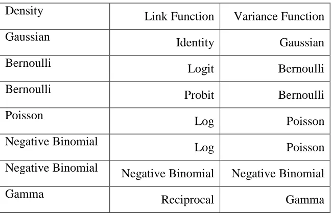
Table 2.2 Common link and variance function combinations ...10

Table 2.3 Link Functions ...11

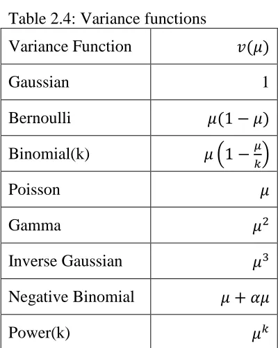
Table 2.4 Variance Functions ...11

Table 3.1 GLM Poisson model with log link ...21

Table 3.2 Penalized GLM Poisson model with log link ...22

Table 3.3 GLM Binomial model with loglog link ...23

Table 3.4 Penalized GLM Binomial model with loglog link...24

Table 3.5 Bootstrap GLM Binomial model with loglog link...25

Table 4.1 Working Correlation Structures ...30

Table 5.1 Results of xtgee model with binomial link and independent working correlation matrix ...39

Table 5.2 Results of estatg ...39

Table 5.3 Results of logit model ...40

Table 5.4 Resilts of fitstat ...41

Table 6.1 Proportion Pan’s QIC identifies correct correlation structure when the true correlation structure is exchangeable ...49

Table 6.2 Proportion modified QIC identifies correct correlation structure when true correlation structure is exchangeable ...49

(12)

Table 6.4 Proportion modified QIC identifies correct correlation structure when true correlation structure is AR(1) ...49

(13)

CHAPTER 1 INTRODUCTION

In the public health field, generalized linear models (GLM) and generalized estimating

equations (GEE) are widely used for analysis of clinical studies and secondary data

analysis. It is important for these researchers to have the necessary tools to analyze and

model their data correctly. This dissertation focuses on a penalized maximum likelihood

estimation method for generalized linear models, measures of association such as the

coefficient of determination and R2 _{for generalized estimating equations, and a modified}

quasi-likelihood information criterion for generalized estimating equations.

Occasionally, problems with convergence of the maximum likelihood arise in

generalized linear models (GLMs). Non-convergence of the maximum likelihood

estimates can result from reasons such as complete separation in the data, extremely large

values that create a difficult situation for convergence, bias, and small sample size. When

one or more of these phenomenon occur during model estimation, researchers are limited

in the ways to deal with this situation. Researchers are even more limited in software if

the response variable is not a binary outcome. Firth’s penalized maximum likelihood

estimation approach is currently only available for binary response models in the most

widely used statistical software programs SAS, R, and Stata.

One of the first steps in estimation of the parameters in a generalized estimating

(14)

equation before maximization. If this matrix is incorrectly specified, efficiency is lost in

the generalized estimating equations estimates. The current criteria for selecting a

working correlation matrix is flawed as in it favors a more simple correlation structure

such as independent correlation matrix. The choice of the independent correlation

structure assumes that the clusters within the data are not correlated. In other words, it

assumes that there is no within group correlation, which we know is normally not the

case in panel, cluster, or longitudinal data.

Often researchers want a measure to show how much variance is explained in the

chosen model. In multiple linear regression, the R2 measure helps researchers with

variable selection and provides a goodness of fit measure for the selected model.

Currently this type of measure is not readily available for models with clustered,

longitudinal or panel data. Non-linear regression models also have pseudo-R2_measures

that are not available for generalized estimating equations models. One difference

between generalized linear models and generalized estimating equations is the

availability of the maximum likelihood. For generalized estimating equation models, the

maximum likelihood is not available, and the quasi-likelihood is used. For pseudo- R2

measures that include the maximum likelihood within the calculation, a different

approach will have to be used.

In this dissertation work, I will accomplish three tasks. First, I will extend a

penalized maximum likelihood estimation method to generalized linear models and

implement the penalized maximum likelihood estimation method in Stata, a statistical

software. Second, I will propose an R2_{and some pseudo-R}2_{measurements for}

(15)

in Stata. Third, I will propose a modified quasi-likelihood information criterion that

identifies the true underlying covariance structure better than the currently available

(16)

CHAPTER 2 GENERALIZED LINEAR MODELS

This chapter presents an introduction to generalized linear models with emphasis on

model building. Common link functions and variance functions are presented and

discussed.

2.1 INTRODUCTION

Generalized Linear Model theory was introduced by Nelder and Wedderburn [1972].

This theory provided a unity for an entire class of regression models. The basis of this

unity is a focus on the single-parameter exponential family of probability distributions.

Member distributions of the exponential family include the normal, Poisson, binomial,

gamma, inverse Gaussian, negative binomial, and geometric distributions. The

exponential family notation which includes a location (mean) parameter and a variance

which is written as a function of the mean times a scalar parameter allows the

specification of models for all exponential family member distributions including those

which are continuous, count, binary, discrete, and proportional outcomes.

The standard linear regression model can be derived from several assumptions.

The first assumption is that each observation of the response variable originates from the

normal distribution: 𝑦_𝑖~𝑁(𝜇_𝑖, 𝜎_𝑖2). The second assumption is that the distributions for all

observations have a common variance: 𝜎_𝑖2 = 𝜎2 for all 𝑖. The third assumption is that

there is a direct relationship between the linear predictor and the expected value of the

(17)

mean, 𝑥𝑖 is a vector of covariates for the 𝑖th observation, and 𝐸(𝑦) = 𝜇 = 𝛽0+ 𝛽1𝑋1+

⋯ + 𝛽_𝑝𝑋_𝑝. The goal of the generalized linear model is to specify the relationship between

the response variable and its’ predictors. Note that the properties of the estimators do not

depend on the assumption of normality.

Generalized linear models are developed by relaxing the assumptions of the

standard linear regression model. An initially nonlinear relationship can be restructured

into a linear relationship through the linear predictor and the mean. Generalized linear

models are defined by the specified distribution (variance function) and the link function.

The assumptions of the generalized linear model as stated by Breslow [1996] are that the

observations are independent, and that the variance function 𝑣(𝜇), the scale factor 𝑎(𝜙),

and the link function are correctly specified, the explanatory variables are in the correct

form, and the residuals have the correct distribution.

2.2 MODEL BUILDING

The components of a generalized linear model are similar to the components of the

standard linear regression model. The first component needed is the response variable, 𝑦,

for which the conditional variance follows that of a distribution belonging to the

exponential family. The second component needed is a linear systematic component (the

linear predictor), 𝜂 = 𝑿𝛽, the product of the parameters 𝛽 and the design matrix 𝑿. The

third component is the link function that relates the linear predictor to the mean. The

fourth component is the variance function 𝑣(𝜇) defining the variance of the response

variable in terms of its mean 𝜇, 𝑉(𝑦) = 𝑎(𝜙)𝑣(𝜇), where 𝑎(𝜙) is the scale factor and the

(18)

Generalized linear models are formulated within the framework of the exponential

family of distributions written as

𝑓𝑦(𝑦; 𝜃, 𝜙) =exp{

𝑦𝜃 − 𝑏(𝜃)

𝑎(𝜙) + 𝑐(𝑦, 𝜙)}

where 𝜃 is the canonical parameter of location and 𝜙 is the parameter of scale. The

canonical parameter relates to the mean and the scalar parameter relates to the variance

for the exponential family members.

Since the observations, 𝑦𝑖, are independent, the joint probability density function

of the sample of n observations, given the parameters 𝜙 and 𝜃, is defined by the product

of the densities of the individual observations. Combining these densities, the joint

probability density function expressed as a function of 𝜙 and 𝜃 given the observations, 𝑦_𝑖

into what is called the likelihood, L, is written as

𝐿(𝜃, 𝜙; 𝑦₁, 𝑦₂, … 𝑦_𝑛) = ∏ exp {𝑦𝑖𝜃𝑖 − 𝑏(𝜃𝑖)

𝑎(𝜙) + 𝑐(𝑦𝑖, 𝜙)}

𝑛

𝑖=1

To obtain estimates of 𝜙 and 𝜃 that maximize the likelihood function, it is easier

to work with the log likelihood,

ℒ(𝜃, 𝜙; 𝑦1, 𝑦2, … 𝑦𝑛) = ∑ {

𝑦_𝑖𝜃_𝑖 − 𝑏(𝜃_𝑖)

𝑎(𝜙) + 𝑐(𝑦𝑖, 𝜙)}

𝑛

𝑖=1

since the values that maximize the likelihood are the same values that maximize the log

likelihood. The canonical parameter is represented by 𝜃, 𝑏(𝜃) is the cumulant, 𝜙 is the

dispersion parameter, and 𝑐() is the normalization parameter. This notation also provides

simple calculations of the first and second derivatives for maximum likelihood estimation

(19)

Each distribution that is part of the exponential family has a unique canonical

link, cumulant, and expectation of the canonical link. Table 2.1 shows 𝜃, 𝑏(𝜃), and 𝑏′_(𝜃)

for members of the single parameter exponential family.

To obtain maximum likelihood estimates, substitute the link function of the linear

predictor for the expected value of the outcome 𝜇. The estimating equation can be written

as

[𝜕𝐿 𝜕𝛽] = 𝑋

𝑇₍𝑦 − 𝐸(𝑦)

𝑎(𝜙) )

1 𝑣(𝐸(𝑦))

𝜕𝑔−1_(𝜂)

𝜕𝜂 = [𝟎𝑝𝑥1]

Here the linear predictor 𝜂 is equated to the canonical link 𝜃. Any monotonic link

function that maps the linear predictor to the range implied to the variance function can

be chosen.

2.3 LINK FUNCTIONS

Each distribution that is a member of the exponential family has compatible link

functions meant to be used under different situations. The Gaussian family model

assumes a normally distributed response variable and generally uses the identity link. The

identity link assumes a continuous response and can take on negative or positive values.

The log-normal model is also based on the Gaussian distribution but uses the log link.

The log link is used for response data that only takes on positive values on the continuous

scale.

The gamma family model is used for modelling outcomes for which the response can

take on only values greater than or equal to zero. This model is generally used with

continuous response data but can also be used with count data where the count data take

the shape of a gamma distribution. The gamma model is compatible with the reciprocal

(20)

can also be used with the identity link to model duration data and assumes there is a

one-to-one relationship between 𝜂 and 𝜇.

The inverse Gaussian distribution is most appropriate to use when modeling a

nonnegative response that has a high initial peak, quick drop, and long right tail or when

modeling discrete data. The log and identity links are commonly used with such

outcomes and are similar to the gamma model.

The binomial-logit family consisting of the Bernoulli/binomial distributions are

used to model discrete or proportional responses. This family can be used to model

number of successes out of a number of trials. The links that are commonly used with this

family are logit, probit, log, complementary log, identity, log, inverse, and

log-complement. The logit link is equivalent to logistic regression where log-odds are

modeled while the probit link is used to model data in terms of normal-based

probabilities. The complementary log-log defines a sigmoid curve where the upper part is

more stretched out than the logit or probit, and the log-log defines a sigmoid curve where

the lower part is more stretched out than the logit or probit. The log link produces

estimates of the log risk ratio, the log-complement estimates log health ratio, and the

identity link yields estimates of the risk difference.

The Poisson family is used to model response variables that are counts or rates.

The identity link measures the rate difference while the log link is used to measure the

difference in the log of the expected incidence rate ratio.

The negative-binomial distribution can also be used to model count outcomes. This

model is useful with overdispersed (relative to the Poisson) count data. It can be derived

(21)

like the Poisson model. The geometric family is the negative-binomial with the scale

parameter 𝜙 equal to 1. The log link for the geometric family also measures incidence

(22)

Table 2.1 Corresponding canonical link, cumulant, and expected value of 𝑦

Distribution 𝜃 𝑏(𝜃) 𝑏′(𝜃)

Binomial 𝑙𝑜𝑔 ( 𝜃

1−𝜃) log (1 + exp(𝜃))

exp (𝜃) 1+exp (𝜃)

Normal 𝜃 𝜃2

2 𝜃

Poisson log (𝜃) exp(𝜃) exp(𝜃)

Inverse Gaussian 1

2𝜃 2

√2𝜃 _√2𝜃1

Gamma 1

𝜃 − log (

1 𝜃)

1 𝜃

Negative Binomial log ( 𝛼𝜃

1+𝛼𝜃)

log (1−exp(𝜃))

𝛼

1 𝛼(

exp (𝜃) 1−exp (𝜃))

Table 2.2: Common link and variance function combinations

Density

Link Function Variance Function

Gaussian _Identity _Gaussian

Bernoulli _Logit _Bernoulli

Bernoulli

Probit Bernoulli

Poisson _Log _Poisson

Negative Binomial

Log Poisson

Negative Binomial _{Negative Binomial} _{Negative Binomial}

Gamma

(23)

Table 2.3: Link functions

Link function 𝜂 = 𝑔(𝜇)

Identity 𝜇

Logit log ( 𝜇

1−𝜇)

Log log (𝜇)

Negative Binomial log ( 𝛼𝜇

1+𝛼𝜇)

Log-complement log (1 − 𝜇)

Log-log −log (− log(𝜇))

Probit Φ−1(𝜇)

Reciprocal 1_𝜇

Table 2.4: Variance functions

Variance Function 𝑣(𝜇)

Gaussian 1

Bernoulli 𝜇(1 − 𝜇)

Binomial(k) 𝜇 (1 −𝜇

𝑘)

Poisson 𝜇

Gamma 𝜇2

Inverse Gaussian 𝜇3

Negative Binomial 𝜇 + 𝛼𝜇

(24)

CHAPTER 3 PENALIZED MAXIMUM LIKELIHOOD APPROACH FOR GENERALIZED LINEAR

MODELS

This chapter discusses a penalized maximum likelihood method for generalized linear

models. The derivation is described and Stata software and examples are displayed.

3.1 INTRODUCTION

This section focuses on the development of a method and its implementation into

statistical software Stata. A new Stata command for estimating generalized linear models

via penalized maximum likelihood is presented. In the past, only a subset of such models

have been available to Stata users through the user-written firthlogit (Coveney

[2008]) command for binomial models (using on the logit link function). The new

firthglm command estimates any generalized linear model supported by the glm

command using penalized log-likelihood.

3.2 CURRENT ISSUES

Firth's penalized maximum likelihood (Firth [1993]) approach was originally developed

to reduce the bias of maximum likelihood estimates. The asymptotic bias of the

maximum likelihood estimate 𝜃̂ can be written as

𝑏(𝜃) =𝑏1(𝜃)

𝑛 +

𝑏₂(𝜃)

𝑛2 + ⋯

Previously two approaches were used to correct for this bias. The Jackknife

(25)

the substitution method. The substitution method substitutes 𝜃̂ for the unknown 𝜃 in

𝑏(𝜃) and gives the second order efficient, bias-corrected estimate as 𝜃̂_𝐵𝐶 = 𝜃̂ − 𝑏1(𝜃̂)

𝑛 .

The jackknife and 𝜃̂𝐵𝐶 are bias-reducing only in an asymptotic sense when 𝜃̂ is infinite.

Both of these methods use a corrective approach rather than a preventive approach.

This bias arises from a combination of the unbiasedness of the score function at

the true value of 𝜃 and the curved nature of the score function. To remove bias from the

maximum likelihood estimator, Firth's method adds a bias correcting term to the score

function. For generalized linear models (GLMs), our target is the canonical parameter of

an exponential family, and in this case, the bias term is simply the Jeffreys invariant

prior. Jeffreys prior removes the bias, and the end result is a penalized log-(pseudo)

likelihood function.

Firth showed that for a random sample from a normal distribution, the

bias-reducing penalty function produces an exactly unbiased estimate for 𝜃 for sample sizes

larger than three. For logisitic regression, the maximum likelihood estimate of 𝛽 is found

to be biased away from the point 𝛽 = 0 which requires bias correction with some degree

of shrinkage of 𝛽 towards this point. When the target parameter is the canonical

parameter of an exponential family, the estimate is second-order efficient, which means

Jeffreys prior is sufficient in removing the bias from the maximum likelihood estimate.

In 2002, Heinze and Schemper claimed that this method developed by Firth was

also useful in solving the problem of separation (Heinze and Schemper [2002]). With

regard to the relationship of a covariate to an outcome variable in a data set, there are

three configurations of 𝑛 observations we can observe: complete separation,

(26)

one or more predictor variables completely. For example, consider a binary outcome

variable and a continuous predictor. If all outcomes with value 1 have corresponding

predictor values less than 4 while all outcomes with value 0 have corresponding predictor

values greater than 6, we have complete separation. In this situation, the maximum

likelihood estimate of the regression parameter on the predictor variable does not exist or

tends to infinity.

Quasi-complete separation exists when the outcome variable separates one or

more predictor variables to a certain point. Consider the previous example of complete

separation where the corresponding predictor values are separated similarly, but now the

predictor values for both outcomes (0 and 1) include the value 5. Here the only

probability to estimate is the probability the predictor value equals 5. All the other

predictor values are separated by the outcome variable. In this situation, the maximum

likelihood estimate of the regression parameter on the predictor variable also does not

exist.

Overlap exists when there is no separation in the data, and this situation is

generally not a problem for parameter estimation. Since there is no separation, the

maximum likelihood estimate exists.

When separation arises, there are a number of options to consider. One can omit

the variable from the model, allowing estimates to be obtained for the other parameters.

By omitting the variable, the information about the effect of the possible risk factor is

lost. One can manipulate the data by using an ad hoc adjustment such as changing cell

frequencies or forcing the largest or smallest observation to have the opposite effect. This

(27)

use exact regression (such as exlogit or expoisson) which replaces the maximum

likelihood estimate by a median unbiased estimate where the estimate of a parameter and

inference are based on the exact null distribution of the sufficient statistic conditional on

the observed values of the other sufficient statistics. This method is useful with one

variable but cannot be used when two or more variables lead to degenerate distributions

of all sufficient statistics.

This penalized maximum likelihood method is currently available for logistic

regression, but these situations are not limited to binary outcomes and can occur for any

specified generalized linear model. In this manuscript we introduce Firth's penalized

maximum likelihood estimation in Section 3.3. In Section 3.4, the Stata syntax is shown

for the new firthglm command, and the examples are contained in Section 3.5.

3.3 METHODS

A bias reduction of maximum likelihood estimates in generalized linear models was

introduced by Firth [1993]. Instead of taking a corrective approach by estimating the

maximum likelihood and then adding a penalty term, Firth modifies the score function

and then produces the maximum likelihood estimate. This is particularly useful when the

maximum likelihood estimate does not exist or is infinite.

The penalized likelihood equation written within the framework of the exponential family

of distributions is defined as

𝐿(𝜃, 𝜙; 𝑦₁, 𝑦₂, … , 𝑦_𝑛) = ∏ exp {𝑦𝑖𝜃𝑖 − 𝑏𝜃𝑖

𝑎(𝜙) + 𝑐(𝑦𝑖, 𝜙)} |𝑖(𝜃)|

1/2 𝑛

(28)

where 𝑦1, 𝑦2, … , 𝑦𝑛 are the sample of independent observations, 𝜃𝑖 is the canonical

location parameter for the 𝑖th observation, 𝜙 is the scale parameter, and |𝑖(𝜃)|1/2 is the

Jeffreys [1946] invariant prior.

We can take the log of equation 2 to obtain the penalized log-likelihood

ℒ(𝜃, 𝜙; 𝑦₁, 𝑦₂, … , 𝑦_𝑛) = ∑ {𝑦𝑖𝜃𝑖 − 𝑏𝜃𝑖

𝑎(𝜙) + 𝑐(𝑦𝑖, 𝜙)} +

1 2log

𝑛

𝑖=1

|𝑖(𝜃)|

since the values that maximize the likelihood also maximize the log-likelihood. The

estimates can then be computed using Stata's ml optimization commands.

Because the likelihood is written in exponential family notation (Hardin and Hilbe

[2011]), we can specify penalized models for not only binary outcomes, but also count,

proportional, discrete, and continuous outcomes.

Firth notes that bias reduction can be affected by the number of factors, especially

the skewness of the maximum likelihood estimate. In this case, one might sacrifice

precision in the estimates. However, in his paper, Firth states that when employing

logistic regression, the maximum likelihood estimate is unbiased and reduces the

variance of the parameter estimates. We are to expect smaller standard errors when using

firthglm. Confidence intervals will be affected since in reality, the estimate's lower

bound should be negative infinity when the maximum likelihood estimate tends to

negative infinity, and the upper bound should be positive infinity when the maximum

likelihood estimate tends to positive infinity.

3.4 STATA SYNTAX

Software accompanying this section includes the command files as well as supporting

(29)

include the usual collection of maximization and display options available to all

estimation commands.

Equivalent in syntax to the to the glm command, the basic syntax for the

penalized generalized linear model is given by

firthglm[𝑑𝑒𝑝𝑣𝑎𝑟 [𝑖𝑛𝑑𝑒𝑝𝑣𝑎𝑟𝑠] ] [𝑖𝑓] [𝑤𝑒𝑖𝑔ℎ𝑡] [ , ∗]

It should be noted, that the penalized log-likelihood maximization method is

implemented using Stata's ml commands specifying the d0 optimization method. As

such, the firthglm command does not support some of the vce()options that are

available in the glm command specifically, the firthglm command does not support

opg, unbiased, robust, or cluster. Similarly, the firthglm command does not

support the pweight option.

Help files are included for the estimation and post-estimation specifications of

these models. The help files include example specifications.

3.5 REAL DATA ANALYSIS

All examples were analyzed using the 12.1 version of Stata (Stata Corp, College Station,

TX). We show two examples in this section. The first example demonstrates bias

reduction when using a Poisson regression. The second example shows how the

penalized maximum likelihood method is useful when there is separation in the data and

the maximum likelihood does not converge. This example uses logistic regression, and

we also compare the firthglm method with bootstrapping.

The first example uses a ship accident dataset from McCullagh and Nelder

[1989], listed on page 205 of the text. This dataset includes the number of reported

(30)

the period of operation, op_00_00, the construction year, co_00_00, and the type of

ship, ship. The exposure in the model is the collective months of service. To better

define some variables, we use the indicator variables op_00_00 to show the starting and

ending years of operation and the indicator variables co_00_00 to show the starting and

ending years of construction. For example, op_70_74 shows whether the ship was in

operation from 1970 to 1974, and co_60_64 shows whether the ship was in

construction from 1960 to 1964. There is a total of 34 full observations in this dataset.

We run a Poisson model of accident on op_75_79, co_65_69,

co_70_74, co_75_79, and ship with a log link. To obtain risk ratios, we use the

eform option.

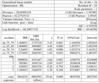
The results of the model are in Table 3.1. The results show that whether the ship

was in service between 1975 and 1979 is a significant predictor of number of accidents.

Also, whether the ship was constructed between 1965 and 1969 or between 1970 and

1974 are also significant predictors of number of accidents. The fourth indicator variable

co_75_79 is not significant with a p-value of 0.052. Ship types 2 and 3 are significantly

different from ship type 1 while ship type 4 and 5 are not significantly different from ship

type 1.

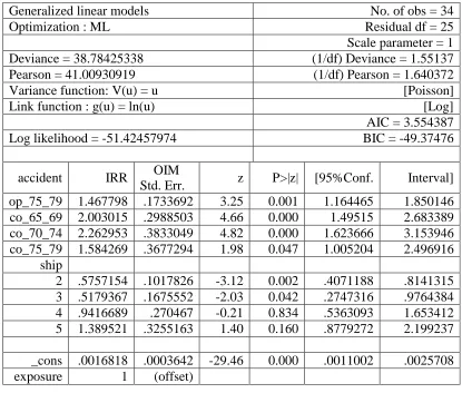
To examine bias reduction, we can run firthglm using the same model options.

From the output in Table 3.2, we can see that the penalized log likelihood of -51.4 is a

good bit smaller than the log likelihood of -68.3. The Aikaike Information Criteria (AIC)

for the penalized maximum likelihood method is smaller than the non-penalized method

(3.55 compared to 4.55). The deviance for the penalized method is slightly larger than the

(31)

for all variables in the model except co_75_79. In the non-penalized GLM model, this

variable was not significant, but is now significant with a p-value of 0.047.

The command firthglm can be applied to any generalized linear model and

canonical link supported by Stata's glm command using penalized log-likelihood. We

illustrate another model using data provided by Dr. José Villa at the USDA-ARS Honey

Bee Breeding, Genetics and Physiology Laboratory (Deroche et al. [2011]) where

convergence is not achieved in a binary response regression model with a log-log link.

Convergence is not achieved due to the issue of complete separation in the data.

These data contain the levels of mite infestation (mites) in a longitudinal study

on bee colonies from nine different genetic origins. Measurements of mite infestation

were recorded every season over a seven year period as well as the status (dead or

alive) of each colony. Here origin 9 and season 4 are the referent groups.

Two genetic origins did not experience any deaths due to the level of mite

infestation (origin 1 and origin 4). This is an example of separation. The effect of

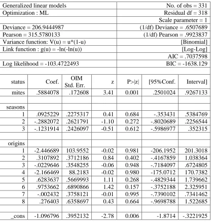
this separation on the model can be seen when using Stata's glm command. We illustrate

a binomial model of status on mites, origin1-origin8, and

season1-season3 with a log-log link. We can see in Table 3.3 that the estimates for origin1

and origin4 are -2.45 and -2.17 with associated standard error estimates which are

approximately 104 and 88. The maximum likelihood estimates of these terms tend toward

negative infinity which implies the odds ratio is tending toward zero. From this model,

we can see that the only significant predictor of status is mites.

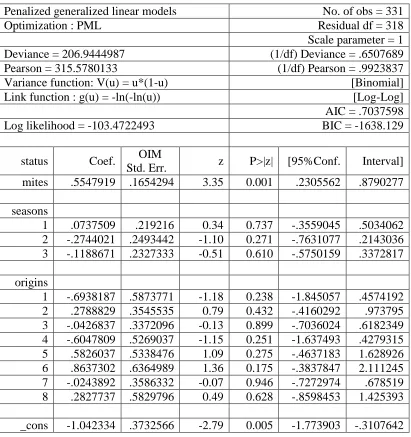
This inability to reach convergence is fixed by estimating a penalized maximum

(32)

link(loglog). The parameter estimates without convergence problems have

estimates and standard errors slightly smaller than those given by glm, but the significant

predictors of status have not changed. These results can be seen in Table 3.4.

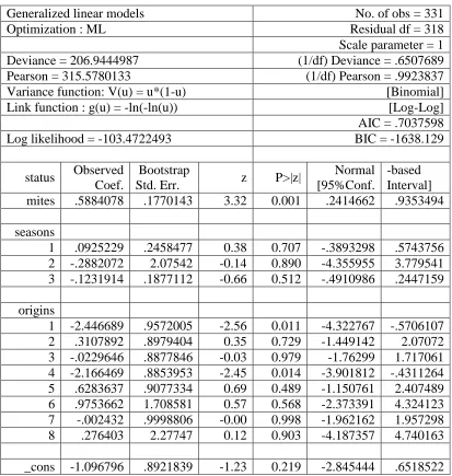
Another alternative to the penalized maximum likelihood method is to use

vce(bootstrap) within the glm model. The results of this method can be seen in

Table 3.5. The standard errors obtained are larger than those obtained through

firthglm but still much smaller than those from glm. The parameter estimates for

origin1 and origin4 are still large, but now they are significant with p-values of

0.011 and 0.014 respectively. Bootstrapping is efficient in giving smaller standard errors,

but in this case, gives misleading results. The option vce(bootstrap) is also

available within the firthglm command.

To explore other options for dealing with separation, we ran a regular logistic

model using family(binomial) and link(logit). We tried to compare this to

using exlogistic, but this method failed to estimate the model and combat the issue

of separation.

3.5 CONCLUSIONS AND DISCUSSIONS

This penalized maximum likelihood method for generalized linear models has

been proven to be useful in bias reduction and solving the problem of separation in data.

In the past, this method was only available in software for a binary outcome using logistic

models. The firthglm command broadens this penalized maximum likelihood method

to all generalized linear models regardless of the structure of the response variable or the

(33)

Table 3.1 GLM Poisson model with log link

gen double exposure = ln(service) 6 missing values generated)

glm accident op_75_79 co_65_69 co_70_74 co_75_79 i.ship, family(poiss) link(log) offset(exposure) eform nolog

Generalized linear models No. of obs = 34

Optimization : ML Residual df = 25

Scale parameter = 1

Deviance = 38.69505154 (1/df) Deviance = 1.547802

Pearson = 42.27525312 (1/df) Pearson = 1.69101

Variance function: V(u) = u [Poisson]

Link function : g(u) = ln(u) [Log]

AIC = 4.545928

Log likelihood = -68.28077143 BIC = -49.46396

accident IRR OIM

Std. Err. z P>|z| [95%Conf. Interval]

op_75_79 1.468831 .1737218 3.25 0.001 1.164926 1.852019

co_65_69 2.008002 .3004803 4.66 0.000 1.497577 2.692398

co_70_74 2.26693 .384865 4.82 0.000 1.625274 3.161912

co_75_79 1.573695 .3669393 1.94 0.052 .9964273 2.485397

ship

2 .5808026 .1031447 -3.06 0.002 .4100754 . 8226088

3 .502881 .1654716 -2.09 0.037 .2638638 .9584087

4 .926852 .2693234 -0.26 0.794 .5244081 1.638141

5 1.384833 .3266535 1.38 0.168 .8722007 2.198762

_cons .0016518 .0003592 -29.46 0.000 .0010786 .0025295

(34)

Table 3.2 Penalized GLM Poisson model with log link

firthglm accident op_75_79 co_65_69 co_70_74 co_75_79 i.ship, family(poiss) link(log) offset(exposure) eform nolog

Scale parameter = 1

Deviance = 38.78425338 (1/df) Deviance = 1.55137

Pearson = 41.00930919 (1/df) Pearson = 1.640372

Variance function: V(u) = u [Poisson]

Link function : g(u) = ln(u) [Log]

AIC = 3.554387

accident IRR OIM

op_75_79 1.467798 .1733692 3.25 0.001 1.164465 1.850146

co_65_69 2.003015 .2988503 4.66 0.000 1.49515 2.683389

co_70_74 2.262953 .3833049 4.82 0.000 1.623666 3.153946

co_75_79 1.584269 .3677294 1.98 0.047 1.005204 2.496916

ship

2 .5757154 .1017826 -3.12 0.002 .4071188 .8141315

3 .5179367 .1675552 -2.03 0.042 .2747316 .9764384

4 .9416689 .270467 -0.21 0.834 .5363093 1.653412

5 1.389521 .3255163 1.40 0.160 .8779272 2.199237

_cons .0016818 .0003642 -29.46 0.000 .0011002 .0025708

(35)

Table 3.3 GLM binomial model with log-log link

glm status mites b4.seasons b9.origins, fam(binomial) link(loglog) nolog

Scale parameter = 1

Deviance = 206.9444987 (1/df) Deviance = .6507689

Pearson = 315.5780133 (1/df) Pearson = .9923837

Variance function: V(u) = u*(1-u) [Binomial]

Link function : g(u) = -ln(-ln(u)) [Log-Log]

AIC = .7037598

status Coef. OIM

mites .5884078 .172608 3.41 0.001 .2501024 .9267133

seasons

1 .0925229 .2275317 0.41 0.684 -.353431 .5384769

2 -.2882072 .2621791 -1.10 0.272 -.8020689 .2256544

3 -.1231914 .2426097 -0.51 0.612 -.5986977 .352315

origins

1 -2.446689 103.9552 -0.02 0.981 -206.1952 201.3018

2 .3107892 .3712186 0.84 0.402 -.4167859 1.038364

3 -.0229646 .3548255 -0.06 0.948 -.7184097 .6724805

4 -2.166469 88.2183 -0.02 0.980 -175.0712 170.7382

5 .6283637 .5669993 1.11 0.268 -.4829344 1.739662

6 .9753662 .6890866 1.42 0.157 -.3752188 2.325951

7 -.002432 .3758121 -0.01 0.995 -.7390102 .7341462

8 .276403 .6358697 0.43 0.664 -.9698788 1.522685

(36)

Table 3.4 Penalized GLM binomial model with log-log link

firthglm status mites b4.seasons b9.origins, fam(binomial) link(loglog) nolog

Penalized generalized linear models No. of obs = 331

Optimization : PML Residual df = 318

Scale parameter = 1

AIC = .7037598

status Coef. OIM

mites .5547919 .1654294 3.35 0.001 .2305562 .8790277

seasons

1 .0737509 .219216 0.34 0.737 -.3559045 .5034062

2 -.2744021 .2493442 -1.10 0.271 -.7631077 .2143036

3 -.1188671 .2327333 -0.51 0.610 -.5750159 .3372817

origins

1 -.6938187 .5873771 -1.18 0.238 -1.845057 .4574192

2 .2788829 .3545535 0.79 0.432 -.4160292 .973795

3 -.0426837 .3372096 -0.13 0.899 -.7036024 .6182349

4 -.6047809 .5269037 -1.15 0.251 -1.637493 .4279315

5 .5826037 .5338476 1.09 0.275 -.4637183 1.628926

6 .8637302 .6364989 1.36 0.175 -.3837847 2.111245

7 -.0243892 .3586332 -0.07 0.946 -.7272974 .678519

8 .2827737 .5829796 0.49 0.628 -.8598453 1.425393

(37)

Table 3.5 Bootstrap GLM binomial model with log-log link

glm status mites b4.seasons b9.origins, fam(binomial) link(loglog) vce(bootstrap) nolog

(running glm on estimation sample) Bootstrap replications (50)

Scale parameter = 1

AIC = .7037598

status Observed Coef.

Bootstrap

Std. Err. z P>|z|

Normal [95%Conf.

-based Interval]

mites .5884078 .1770143 3.32 0.001 .2414662 .9353494

seasons

1 .0925229 .2458477 0.38 0.707 -.3893298 .5743756

2 -.2882072 2.07542 -0.14 0.890 -4.355955 3.779541

3 -.1231914 .1877112 -0.66 0.512 -.4910986 .2447159

origins

1 -2.446689 .9572005 -2.56 0.011 -4.322767 -.5706107

2 .3107892 .8979404 0.35 0.729 -1.449142 2.07072

3 -.0229646 .8877846 -0.03 0.979 -1.76299 1.717061

4 -2.166469 .8853953 -2.45 0.014 -3.901812 -.4311264

5 .6283637 .9077334 0.69 0.489 -1.150761 2.407489

6 .9753662 1.708581 0.57 0.568 -2.373391 4.324123

7 -.002432 .9998806 -0.00 0.998 -1.962162 1.957298

8 .276403 2.27747 0.12 0.903 -4.187357 4.740163

(38)

CHAPTER 4 GENERALIZED ESTIMATING EQUATIONS

This chapter introduces generalized estimating equations and its link to generalized linear

models. The extension of the working correlation matrix is discussed and the

quasi-likelihood is introduced.

4.1 INTRODUCTION

One vital assumptions of generalized linear models is independence of the observations.

This assumption is violated when the data may be grouped in some manner such as

patients from the same hospital or when multiple observations are made on the same

subject over time. There are multiple ways to address clustered, panel or longitudinal

data, and each method has its own advantages and limitations. The naïve way to address

this type of data is to ignore the panel structure of the data yielding a pooled

(independence) estimator. This method results in a consistent estimator but one that is not

efficient leading to (possibly) unreliable standard error estimates. Another way to address

panel data is to include an effect for each panel in the estimating equation. This method

allows fixed or random effects and conditional or unconditional effects. When the data

include a finite number of panels in a population where each panel is represented in the

sample, it is more reasonable to consider an unconditional fixed effects estimator.

However, if there exists an infinite number of panels in the population, it is more

reasonable to consider a conditional fixed effects estimator. Here one can include a fixed

(39)

model conditions out the fixed effects from the estimation leading to a log-likelihood

which does not depend on the fixed effects. Here one can make inferences about

population averages and where the mean response is conditional only on covariates. Also

known as subject-specific models, the random effects model allows regression

coefficients (intercept and slope) to vary from person to person according to a random

effects distribution. The transitional Markov model represents the probability distribution

at each time point as conditional on the previous time point and is usually estimated using

Gibbs sampling. An increasingly popular alternative introduced by Liang and Zeger

[1986] is known as Generalized Estimating Equations.

4.2 EXTENSION OF GENERALIZED LINEAR MODELS

In their manuscript, Liang and Zeger [1986] provide an extension to generalized linear

models which they refer to as population-averaged generalized estimating equations. This

method induces an interpretation of the coefficients as population averages and

introduces the dependency (non-independence) of the observations directly into the

estimating equation of the pooled estimator. The estimating equation in a generalized

linear model which assumes independence can be written as

[𝜕𝐿 𝜕𝛽] = ∑ 𝑋𝑖 𝑇_𝐷 𝑛 𝑖=1 (𝜕𝑔 −1_(𝜂 𝑖) 𝜕𝜂_𝑖 ) (𝑣(𝐸(𝑦𝑖)))

−1₍𝑦𝑖 − 𝐸(𝑦𝑖)

𝑎(𝜙) ) = ∑ 𝑋_𝑖𝑇𝐷 𝑛 𝑖=1 (𝜕𝑔 −1_(𝜂 𝑖) 𝜕𝜂_𝑖 ) (𝑣(𝐸(𝑦𝑖))

−1₂

)

𝑇

𝐼(𝑛_𝑖)𝑣(𝐸(𝑦_𝑖))−

1

2₍𝑦𝑖 − 𝐸(𝑦𝑖)

𝑎(𝜙) )

where 𝐼(𝑛_𝑖) is the identity matrix representing the within-group correlation (assumed to

be independent). One can parameterize an alternative correlation matrix to model the

within-group correlation structure by replacing the identity matrix with a working

(40)

[𝜕𝐿 𝜕𝛽] = ∑ 𝑋𝑖 𝑇_𝐷 𝑛 𝑖=1 (𝜕𝑔 −1_(𝜂 𝑖) 𝜕𝜂𝑖 ) (𝑣(𝐸(𝑦𝑖)) −1₂

)

𝑇

𝑅(𝛼)𝑣(𝐸(𝑦𝑖)) −1₂

(𝑦𝑖 − 𝐸(𝑦𝑖)

𝑎(𝜙) )

where 𝛼 is a vector of parameters through which the matrix 𝑅 is structurally constrained

to represent the working or within-panel correlation. Here it is shown that the focus of the

generalized estimating equation is on the marginal distribution and the estimator which

sums the panel-level contribution to the estimating equations after accounting for the

within-panel correlation. Thus, the estimating equation for the regression parameters 𝛽

are formed for the average (sum) of the panels.

4.3 WORKING CORRELATION STRUCTURE

The researcher or analyst is charged with making the correct structural choice of the

working correlation matrix for models estimated using generalized estimating equations.

There are several correlation structure choices available in software. The most commonly

used correlation structures are the independent, exchangeable, autoregressive(1), and

unstructured. These structures are illustrated in Table 4.1.

Consider independent observations from 𝑛 individuals. For each individual 𝑖, a

response 𝑦_𝑖𝑡 and a 𝑝 × 1 covariate vector 𝑥_𝑖𝑡 = (𝑥_𝑖𝑡1, 𝑥_𝑖𝑡2, … , 𝑥_𝑖𝑡𝑝)𝑇 are gathered at

times 𝑡 = 1, 2, … , 𝑚_𝑖. Let 𝑌_𝑖 = (𝑦_𝑖1, 𝑦_𝑖2, … , 𝑦_𝑖𝑚_𝑖)𝑇_{be the}_𝑚

𝑖× 1 vector of responses for

the 𝑖𝑡ℎ individual and 𝑋𝑖 = (𝑥𝑖1𝑇, 𝑥𝑖2𝑇, … , 𝑥𝑖𝑚𝑖

𝑇 ₎𝑇_{be the}_𝑚

𝑖 × 𝑝 corresponding covariate

matrix. The working correlation structure is chosen for the full model prior to the model

selection of the number of covariates.

4.4 QUASI-LIKELIHOOD

The quasi-likelihood is constructed for the mean parameter 𝜇 = 𝐸(𝑦) and the dispersion

(41)

probability distribution. McCullagh and Nelder (1989) give the log quasi-likelihood

based on the model specification 𝐸(𝑦) = 𝜇 and 𝑣𝑎𝑟(𝑦) = 𝜙𝑣(𝜇) as

𝑄(𝜇, 𝜙; 𝑦) = ∫ 𝑦 − 𝑡

𝜙𝑣(𝑡)𝑑𝑡

𝜇

𝑦

The quasi-likelihood can be written as a function of the regression coefficients 𝛽, for

example 𝑄(𝛽, 𝜙; (𝑦, 𝑥)) = 𝑄(𝑔−1_{(𝑥𝛽), 𝜙; 𝑦)}_{. If it is assumed that the working}

independence model 𝑅 = 𝐼 is selected, then the paired observations (𝑌_𝑖𝑗, 𝑋_𝑖𝑗) in the data

𝐷 are independent. Then the quasi-likelihood based on 𝐷 is

𝑄(𝛽, 𝜙; 𝐼, 𝐷) = ∑ ∑ 𝑄 (𝛽, 𝜙; (𝑌_𝑖𝑗, 𝑋_𝑖𝑗)) .

𝑛𝑖

𝑗=1 𝑛

𝑖=1

Then the quasi-deviance can be defined as

𝐷𝑒𝑣𝑖𝑎𝑛𝑐𝑒 = 2 ∫ 𝑦 − 𝜇

𝑣(𝜇) 𝑑𝜇

𝑦

𝜇 ̂

.

The quasi-likelihood can also be written in terms of the quasi-deviance as

𝑄(𝑀) = ∑ ∑ 𝑄 (𝛽, 𝜙; (𝑌_𝑖𝑗, 𝑋_𝑖𝑗)) = −𝐷𝑒𝑣(𝑀)

2

𝑛𝑖

𝑗=1 𝑛

𝑖=1

(42)

Table 4.1 Working Correlation Structures

Working correlation structure Example

3 x 3 matrix

Independent: 𝐶𝑜𝑟𝑟(𝑦_𝑖𝑗, 𝑦_𝑖𝑘) = {1 𝑗 = 𝑘

0 𝑗 ≠ 𝑘 [

1 0 0

0 1 0

0 0 1

]

Exchangeable: 𝐶𝑜𝑟𝑟(𝑦𝑖𝑗, 𝑦𝑖𝑘) = {

1 𝑗 = 𝑘

𝛼 𝑗 ≠ 𝑘 [

1 𝛼 𝛼

𝛼 1 𝛼

𝛼 𝛼 1

]

AR-1: 𝐶𝑜𝑟𝑟(𝑦_𝑖𝑗, 𝑦_𝑖𝑘) = 𝛼|𝑗−𝑘| [

1 𝛼 𝛼2

𝛼 1 𝛼

𝛼2 _𝛼 ₁

]

Unstructured: 𝐶𝑜𝑟𝑟(𝑦𝑖𝑗, 𝑦𝑖𝑘) = {

1 𝑗 = 𝑘 𝛼𝑚𝑖𝑛(𝑗,𝑘),max (𝑗,𝑘) 𝑗 ≠ 𝑘 [

1 𝛼₁₂ 𝛼₁₃

𝛼12 1 𝛼23

𝛼₁₃ 𝛼₂₃ 1

(43)

CHAPTER 5 R

2AND PSEUDO-R2 FOR GENERALIZED ESTIMATING EQUATIONS

This chapter introduces the R2_{and pseudo-R}2_{statistics currently available for generalized}

linear models. The likelihood is replaced with the quasi-likelihood and a post estimation

command for Stata is introduced.

5.1 INTRODUCTION

For generalized linear models, there are many model measures (diagnostic criteria) that

are not available for generalized estimating equation models. One of these measures is

the coefficient of determination 𝑅2. Natarajan, et.al [2007] proposed a measure of partial

association for GEE and a coefficient of determination to measure the strength of

association between the outcome variable and the fitted values based on the estimated

coefficients. The psuedo-R2 statistics to be explored are Efron’s psuedo-R2 (for

continuous and binary outcomes) [1978], McFadden’s likelihood ratio index (for any

outcome) [1974], Ben-Akiva and Lerman’s adjusted likelihood ratio index (for any

outcome) [1985], Cox and Snell [1968] and Maddala [1983] combined transformation of

likelihood ratio (for any outcome), and Cragg and Uhler’s normed measure (for any

outcome) [1970]. Where the likelihood is used for a calculation, GEE’s quasi-likelihood

calculation will be inserted.

5.2 CURRENT AVAILABILITY OF R2 IN GENERALIZED LINEAR MODELS

The most commonly used R2 is the one that involves the calculation of residual sum of

(44)

variance explained and is written as

𝑅2 _{= 1 −}∑ (𝑦𝑖− 𝑦̂𝑖) 2 𝑛

𝑖=1

∑𝑛𝑖=1(𝑦𝑖 − 𝑦̅)2

.

It can also be interpreted as the squared correlation and the ratio of variances. The

numerator is in terms of the differences of the observed and fitted values, while the

denominator is in terms of the differences of the observed and mean values.

The above measure is used for linear regression. When these types of statistics are

applied to generalized linear models, they are called pseudo-𝑅2 statistics. Other measures

are available for models other than linear regression. The ones discussed herein are

Efron’s pseudo-𝑅2, McFadden’s likelihood ratio index, Ben-Akiva and Lerman adjusted

likelihood ratio index, Cragg and Uhler normed measure, and the Cox-Snell or

transformation of likelihood ratio.

Efron [1978] defines a measure as an extension to the regression model’s

“percent variance explained” interpretation and is given by

𝑅_{𝐸𝑓𝑓𝑟𝑜𝑛}2 = 1 −∑ (𝑦𝑖 − 𝜇̂𝑖)

2 𝑛

𝑖=1

∑𝑛𝑖=1(𝑦𝑖− 𝑦̅)2

where 𝜇̂ is the model predicted probabilities. This measure was originally directed at

binary outcome models, but can also be used for continuous models by replacing the 𝜇̂_𝑖

with 𝑦̂_𝑖.

McFadden [1974] defines a measure, sometimes called the likelihood-ratio index,

as another extension to the “percent variance explained interpretation” given by

(45)

where ℒ is the log-likelihood, 𝑀_𝛼 is the model with only an intercept, and 𝑀_𝛽 is the

model with intercept and covariates.

Ben-Akiva and Lerman [1985] extended McFadden’s pseudo-𝑅2 to include an

adjustment for the number of parameters in the model. This adjustment is similar to the

adjusted 𝑅2 in linear regression and is given by the formula

𝑅_{Ben−Akiva&Lerman}2 = 1 −ℒ(𝑀𝛽) − 𝑝 ℒ(𝑀_𝛼)

where 𝑝 is the number of parameters in the model. The intention behind the adjustment is

to decrease the likelihood so that non-significant variables included in the model do not

cause a significant increase in the criterion measure.

By combining the work of Cox and Snell [1968] and Maddala [1983], a maximum

likelihood pseudo-𝑅2 is described in the formula

𝑅_ML2 = 1 − {𝐿(𝑀𝛼) 𝐿(𝑀_𝛽)}

2 𝑛

= 1 − exp (−𝐺

2

𝑛)

where 𝐺2 = −2 ln{𝐿(𝑀𝛼)

𝐿(𝑀𝛽)}. This measure is an extension to the transformation of the

likelihood ratio.

The last measure examined here is the Cragg and Uhler [1970] normed measure.

Cragg and Uhler introduced a transformation of the likelihood ratio pseudo-𝑅2 because

the 𝑅_ML2 does not approach 1 as the fit of the two comparison models converge. The

normed version of the 𝑅_ML2 is given by

𝑅_Cragg&Uhler2 = 𝑅ML

2

max𝑅_ML2 =

1 − {𝐿(𝑀𝛼) 𝐿(𝑀_𝛽)}

2 𝑛

(46)

These pseudo-𝑅2 measures are available in a user-written Stata command named

fitstat. The command fitstat is a post estimation command that calculates the

McFadden, Ben-Akiva and Lerman (adjusted McFadden), Cox-Snell, Cragg-Uhler, and

Efron pseudo-𝑅2 measures after computing the clogit, cloglog, intreg,

logisitic, logit, mlogit, nbreg, ocratio, ologit, oprobit, poisson,

probit, regress, tnbreg, tpoisson, zinb, zip, or ztb regression models. The

fitstat command was developed by Long and Freese [2014].

5.3 GENERALIZED LINEAR MODEL R2EXTENSION TO GENERALIZED ESTIMATING

EQUATIONS

Natarajan, et.al [2007] proposed a measure of partial association for GEE and a

coefficient of determination to measure the strength of association between the outcome

variable and all of the coefficients. Using ordinary least squares (OLS) to estimate the

regression parameters allows the estimate of the partial correlation coefficient to be a

monotone function of the Z-statistic that is used to test whether a single regression

coefficient is equal to zero. Natarajan, et. al. propose to use the transformation of the

GEE Z-statistic as a measure of partial association. Following this same thought, they

propose to use a function of the Wald statistic that tests whether all parameters (except

the intercept) are equal to zero to generate the coefficient of determination.

For clustered data, each individual 𝑖(𝑖 = 1, … , 𝑁) has an 𝑛_𝑖x1 response vector

𝑌_𝑖 = [𝑌_𝑖1, … , 𝑌_𝑖𝑛_𝑖]𝑇 and a Kx1 covariate vector 𝑥_𝑖𝑗 = [𝑥_𝑖𝑗1, … , 𝑥_𝑖𝑗𝐾]𝑇. To calculate 𝛽

estimates through a GEE approach, the equation below is solved iteratively.

𝑆(𝛽; 𝑅, 𝐷) ≡ ∑ 𝐷_𝑖′𝑉_𝑖−1(𝑌_𝑖 − 𝜇_𝑖) = 0

𝑛

𝑖=1

(47)

where 𝐷_𝑖 = 𝐷_𝑖(𝛽) =𝜕𝜇𝑖(𝛽)

𝜕𝛽′ and 𝑉𝑖 is a working covariance matrix of 𝑌𝑖. The working

correlation matrix 𝑅 = 𝑅(𝛼) can be expressed in terms of 𝑉_𝑖 = 𝐴1/2_𝑖 𝑅(𝛼)𝐴1/2_𝑖 , where 𝐴_𝑖

is a diagonal matrix with elements 𝑣𝑎𝑟(𝑌𝑖𝑗) = 𝜙𝑣(𝜇𝑖𝑗), which is specified as a function

of the mean 𝜇_𝑖𝑗 = 𝐸(𝑌_𝑖𝑗|𝑥_𝑖𝑗) = 𝑔(𝑥_𝑖𝑗′𝛽). The parameter 𝛼 represents a vector of some

unknown parameters involved in estimating the working correlation structure.

The GEE Wald Z-statistic to test 𝐻₀: 𝛽_𝐾 = 0 is calculated using the estimate of

the 𝛽̂_𝐾 and dividing it by the model-based standard error estimate of 𝛽̂_𝐾; √𝑉𝑎𝑟̂ (𝛽̂_𝐾) .

Since the Wald statistic has been shown to have poor properties as |𝛽̂𝐾| gets large, they

propose to use the Wald statistic with the variance of 𝛽̂_𝐾 estimated under the null

𝐻₀: 𝛽_𝐾 = 0 by replacing 𝑉𝑎𝑟̂ (𝛽̂_𝐾) with the GEE robust variance estimate 𝑉𝑎𝑟̃ (𝛽̂_𝐾). This

gives a measure of partial association which under the null is approximately chi-square

with 1 degree of freedom.

𝑍̃ =_𝐾 𝛽̂𝐾

√ 𝑉𝑎𝑟̃ (𝛽̂𝐾)

We then can define the measure of partial association between 𝑌_𝑖𝑗 and 𝑥_𝑖𝑗𝐾 to be

𝜌̃ =_𝐾 𝑧̃𝐾/√𝑁 √1 + 𝑧̃_𝐾2_/𝑁

which ranges from -1 to 1.

For the GEE model, 𝐸(𝑌_𝑖𝑗|𝑥_𝑖𝑗) = 𝑔(𝑥_𝑖𝑗′𝛽_𝐾), the Wald test to test 𝐻₀: 𝛽₁ = ⋯ =

𝛽_𝐾 = 0 can be used to form an 𝑅2_{statistic. Following the above derivation of the}

measure of partial association, it is proposed that the coefficient of determination be

(48)

𝑅̃ =2 𝑄̃/𝑁

1 + 𝑄̃/𝑁

where

𝑄̃ = [𝐶𝛽̂]′[𝐶 𝑉𝑎𝑟̃ (𝛽̂_𝐾)𝐶′]−1[𝐶𝛽̂],

is the Wald statistic with the GEE robust covariance matrix estimated under the null. This

statistic will range from 0 to 1 but does not guarantee that a model with more covariates

would have a larger 𝑅̃2_{. This is shown by Natarajan et al. when an additional covariate}

adds very little information.

In order to generalize the pseudo-𝑅2 measures discussed in section 5.3 to

generalized estimating equations, the maximum likelihood calculations must be replaced

with the quasi-likelihood calculations. The extended measures for 𝑅_McFadden2 is now

𝑔𝑅_McFadden2 = 1 −𝑄(𝑀𝛽) 𝑄(𝑀_𝛼)

where 𝑄(𝑀_𝛼) is the quasi-likelihood for the model with only an intercept and 𝑄(𝑀_𝛽) is

the model with intercept and predictors. The quasi-likelihood can also be written in terms

of the quasi-deviance as

𝑄(𝑀) = ∑ ∑ 𝑄 (𝛽, 𝜙; (𝑌_𝑖𝑗, 𝑋_𝑖𝑗)) = −𝐷𝑒𝑣(𝑀)

2

𝑛𝑖

𝑗=1 𝑛

𝑖=1

where 𝐷𝑒𝑣(𝑀) = 2 ∫_𝜇_̂𝑦𝑦−𝜇_𝑣(𝜇)𝑑𝜇. The extended measure for 𝑅_{Ben−Akiva&Lerman}2 is then

given by

𝑔𝑅_{Ben−Akiva&Lerman}2 = 1 −𝑄(𝑀𝛽) − 𝑝

𝑄(𝑀_𝛼) .

Similar replacements are made for 𝑅_ML2 _and_𝑅

(49)

𝑔𝑅_ML2 = 1 − {𝑄(𝑀𝛼) 𝑄(𝑀𝛽) } 2 𝑛 and

𝑔𝑅_Cragg&Uhler2 = 𝑔𝑅ML

2

max𝑔𝑅_ML2 =

1 − {𝑄(𝑀𝛼) 𝑄(𝑀_𝛽)}

2 𝑛

1 − 𝑄(𝑀𝛼)2/𝑛

.

In Efron’s pseudo-𝑅2, we replace the single summand for observations with a double

summand to account for the panel observations and within a panel. The generalized Efron

pseudo-𝑅2 can be written as

𝑔𝑅_Efron2 = ∑ ∑ (𝑦𝑖𝑗− 𝑦̂𝑖𝑗)

2 𝑛𝑖 𝑗=1 𝑛 𝑖=1 ∑ ∑ (𝑦𝑖𝑗 − 𝑦̅) 2 𝑛𝑖 𝑗=1 𝑛 𝑖=1

These calculations were made available in Stata in a user-written, post-estimation

command named estatg. This command is available after any GEE model is estimated

in Stata. The post-estimation command works for any link and variance function.

5.4 REAL DATA ANALYSIS

To test the extensions of the pseudo-𝑅2 measures in GEE models, one can compare the

quasi-likelihood pseudo-𝑅2_{measures to the likelihood based pseudo- pseudo-}_𝑅2

measures with a sample dataset. We used a dataset on low birthweight from Homer and

Lemeshow (2013) in Stata. There are a total of 189 observations in this dataset. This

dataset includes an identification code for each mother, an indicator variable of low birth

weight (low), the age of the mother (age), the categorical variable race (race), an

indicator variable of whether or not the mother smoked during pregnancy (smoke), the

mother’s pre-pregnancy weight (lwt), an indicator variable of whether or not the mother

(50)

birth had uterine irritability (ui). We run a logistic model (link function as binomial and

variance function as independent) on age, lwt, race, smoke, ptl, ht, and ui on

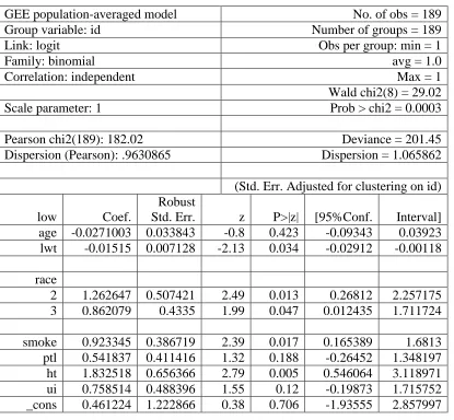
low. The xtgee model fit is shown in Table 5.1 where it is shown that lwt, race,

smoke, and ht are significant predictors of low. The output from estatg is given in

Table 5.2 for the GEE 𝑅2 and the five pseudo-𝑅2.

We can compare this to the output of fitstat after running a logit model

and see that the replacement of the maximum likelihood with the quasi-likelihood works

well in this situation. When fitting the same model under GLM and independent GEE, we

have the same results. The results of the logit model in Table 5.3 show that lwt,

race, smoke, and ht are significant predictors of low. The results of fitstat in

Table 5.4 match the results of estatg found in Table 5.2. Note that the GEE -𝑅2

measure is not available in the output of fitstat since this measure is specifically

designed for GEE models.

5.5CONCLUSION AND DISCUSSION

The 𝑅2 measure is a popular goodness of fit statistic that was not made available for GEE

models. By building on other pseudo-𝑅2_{measures and writing them in terms of the}

quasi-likelihood instead of the maximum likelihood, we have made an important statistic

that will be available in Stata for longitudinal, clustered, or panel data. Researchers can

now get a measure of the variance explained in a GEE model. The GEE 𝑅2 measure will

(51)

Table 5.1 Results of xtgee model with binomial link and independent working correlation

xtset id

xtgee low age lwt i.race smoke ptl ht ui, family(binomial) robust corr(ind)nolog

GEE population-averaged model No. of obs = 189

Group variable: id Number of groups = 189

Link: logit Obs per group: min = 1

Family: binomial avg = 1.0

Correlation: independent Max = 1

Wald chi2(8) = 29.02

Scale parameter: 1 Prob > chi2 = 0.0003

Pearson chi2(189): 182.02 Deviance = 201.45

Dispersion (Pearson): .9630865 Dispersion = 1.065862

(Std. Err. Adjusted for clustering on id)

low Coef.

Robust

age -0.0271003 0.033843 -0.8 0.423 -0.09343 0.03923

lwt -0.01515 0.007128 -2.13 0.034 -0.02912 -0.00118

race

2 1.262647 0.507421 2.49 0.013 0.26812 2.257175

3 0.862079 0.4335 1.99 0.047 0.012435 1.711724

smoke 0.923345 0.386719 2.39 0.017 0.165389 1.6813

ptl 0.541837 0.411416 1.32 0.188 -0.26452 1.348197

ht 1.832518 0.656366 2.79 0.005 0.546064 3.118971

ui 0.758514 0.488396 1.55 0.12 -0.19873 1.715752

(52)

Table 5.2 Results of estatg

Pseudo-R2 measures for GEE models

GEE Efron McFadden Ben-Akiva

Lerman

Cox Snell

Cragg Uhler

0.1331 0.1642 0.1416 0.0649 0.1612 0.2267

Table 5.3 Results of logit model

logit low age lwt i.race smoke ptl ht ui nolog

Logistic regression Number of obs = 189

LR chi2(8) = 33.22 Prob > chi2 = 0.0001

Log likelihood = -100.724 Pseudo R2 = 0.1416

low Coef. Std. Err. z P>|z| [95%Conf. Interval]

age -0.0271 0.03645 -0.74 0.457 -0.09854 0.044341

lwt -0.01515 0.006926 -2.19 0.029 -0.02873 -0.00158

race

2 1.262647 0.52641 2.4 0.016 0.230902 2.294392

3 0.862079 0.439153 1.96 0.05 0.001355 1.722804

smoke 0.923345 0.400827 2.3 0.021 0.137739 1.708951

ptl 0.541837 0.346249 1.56 0.118 -0.1368 1.220472

ht 1.832518 0.691629 2.65 0.008 0.476949 3.188086

ui 0.758514 0.459377 1.65 0.099 -0.14185 1.658875

Lists in a Lighthouse

Scholar Commons

Diagnostics and Model Selection for Generalized

Linear Models and Generalized Estimating

Equations

DIAGNOSTICS AND MODEL SELECTION FOR GENERALIZED

LINEAR MODELS AND GENERALIZED ESTIMATING EQUATIONS

DEDICATION

ACKNOWLEDGEMENTS

ABSTRACT

TABLE OF CONTENTS

LIST OF TABLES

CHAPTER 1

INTRODUCTION

CHAPTER 2

GENERALIZED LINEAR MODELS

CHAPTER 3

PENALIZED MAXIMUM LIKELIHOOD APPROACH FOR GENERALIZED LINEAR

MODELS

CHAPTER 4

GENERALIZED ESTIMATING EQUATIONS

CHAPTER 5

R