Improving Image Deblurring Using Genetic Algorithm

(1)

ISSN (Print) : 2320 – 3765 ISSN (Online): 2278 – 8875

I

nternational

J

ournal of

A

dvanced

R

esearch in

E

lectrical,

E

lectronics and

I

nstrumentation

E

ngineering

(An ISO 3297: 2007 Certified Organization)

Vol. 5, Issue 7, July 2016

Improving Image Deblurring Using Genetic

Algorithm

Prof. S.M. Ali1, Ruqaiya Begum2

Associate Professor, Dept. of ECE, Anjuman College of Engineering and Technology Nagpur, India1 PG Student, Dept. of ECE, Anjuman College of Engineering and Technology Nagpur, India2

ABSTRACT: When we use a camera to click a picture, we want the clicked image to be a exact representation of the scene that we see—but every image is more or less blurry. Thus, image deblurring is fundamental in making pictures sharp and useful. A digital image is made of picture elements called pixels. Each pixel is assigned an intensity, meant to characterize the color of a small rectangular segment of the scene. A small picture typically has around 2562 = 65536 pixels while a high-resolution picture often has 5 to 10 million pixels. Some blurring always arises in the recording of a digital image, because it is unavoidable that scene information “spills over” to neighboring pixels. For example, the optical system in a camera lens may be out of focus, so that the incoming light is smeared out. The same problem arises, for example, in astronomical imaging where the incoming light in the telescope has been slightly bent by turbulence in the atmosphere. In these and similar situations, the expected result is that we record a blurred image.

In image deblurring, we want to recover the unique, sharp image by using a mathematical model of the blurring process. The issue is that some information on the lost details is present in the blurred image—but this information is “hidden” and can only be improved if we know the details of the blurring process. unhappily there is no hope that we can recover the original image exactly! This is due to various unavoidable errors in the recorded image. The most important errors are approximation errors and ﬂuctuations in the recording process when representing the image with a

limited number of digits. The effect of this noise puts a limit on the size of the details that we can hope to recover in the reconstructed image, and the limit depends on both the noise and the blurring process. Keywords—component; formatting; style; styling; insert (key words)

KEYWORDS: Keywords—component; formatting; style; styling; insert (key words)

I.INTRODUCTION

Image deblurring(ID) is a problem where the observed image is produced as the convolution of a sharp image with a blur filter, possibly along with some noise (assumed spectrally white and Gaussian). With applications in many areas (e.g. photography, surveillance, remote sensing, medical imaging, astronomy), research on ID can be split into non-blind ID (NBID), in which the blur filter is assumed familiar, and (real) blind ID (BID), in which both the image and the blur filter are (totally or partly) are not familiar. Despite its narrower applicability, NBID is already a challenging problem to which a large amount of research has been (and still is) devoted, mainly due to the ill-conditioned nature of the blur operator: the observed image does not uniquely and stably determine the underlying original image [38]. If this problem is serious with a known blur, it is much worse if there is even a slight mismatch between the assumed blur and the true one. Most of the NBID methods overcome this difficulty through the use of an image regularizes, or prior, the weight of which has to be tuned or adapted. Most state-of-the-art regularizes exploit the sparsity1 of the high frequency/edge components of images; this is the rationale underlying wavelet/frame-based methods and total variation (TV) regularization. With application not only in ID, but also in other inverse problems, several optimization techniques have been proposed to handle scarcity-inducing regularizes.

(2)

I

nternational

J

ournal of

A

dvanced

R

esearch in

E

lectrical,

E

lectronics and

I

nstrumentation

E

ngineering

use of priors/regularizes. In contrast, a recent BID method does not use prior knowledge about the blur, yet achieves state of-the-art performance on a huge range of synthetic and real problems. That method is iterative and starts by supposing the main features of the image, using a large regularization weight, and gradually learns the image and filter details, by slowly decreasing the regularization parameter. From an optimization point of view, this can be seen as a continuation method designed to obtain a good local minimum of the underlying non-convex objective function.

The disadvantage of the technique is that it is not automatic but it requires manual stopping, which corresponds to choosing the final value of the regularization parameter. In fact ,adjusting the regularization parameter and/or finding robust stopping criteria for iterative (blind or not) ID algorithms is along standing, but still open, research area .A crucial issue in the regularization of ill-posed inverse problems is the choice of the regularization factor, a subject to which much work has been devoted. The discrepancy principle (DP) chooses the regularization factors that the variance of the residual equals that of the noise; the DP thus requires an accurate estimate of the noise variance and is known to yield over-regularized estimates. A recent extension of the DP uses not only the variance, but also other residual moments. Local residual information have also been used to obtain locally adaptive TV regularizes for NBID.

II.IMAGE DEBLURRING

ID can be split into non-blind ID (NBID), in which the blur filter is assumed familiar, and (real) blind ID (BID), in which both the image and the blur filter are (totally or partly) are not familiar.

A .Non-blind Deblurring

In NBID, h is assumed to be known and the cost function (2) is reduced with respect to x, given some of the regularization factor λ. Many optimization methods for ID decrease the cost function (2) iteratively compute the picture estimate at iteration t+1 as a reason of the previous estimate xt, the available data (y and h), and the regularization parameter λ:

xk+1 = f(xk, y, h, λ). (3) Besides requiring a good estimate for the regularization parameter λ, these iterative approaches also need stopping criteria, which considerably influence the final results. For fairness, it should be mentioned that some high-tech methods don’t fall in the category of methods mentioned in the previous paragraph. For example, the method proposed in[16] (arguably the method yielding the current best results) isiterative, but rather than look for a minimize of an objective function, it looks for equilibrium between two objective functions. Other NBID methods are not based on iterative minimization of objective functions.

B .Blind Deblurring

In BID, both the image and the filter are not familiar. A BID problem suffers from an obvious scarcity of data, since there are many pairs (x, h) that explain equally well the observed data y. Most BID methods circumvent this difficulty by adding to (2) a regularizer on the blur filter and, usually, by alternatingly estimating the image and the blur filter. A regularizer on the blur naturally involves an supplementary regularization parameter, also requiring alteration, while the alternating estimation of the image and the filter requires good initialization (since the underlying objective (2) is non-convex) and a good criterion to stop the iterative process.

III.GENETIC ALGORITHM

In the existing system the researchers have focused on estimation of parameters for blind and non blinded blurring which causes inherent time delay in estimation of residual whiteness measures. Thus the system speed in reduced and overall system accuracy is compromised. Our approach will be to reduce the system time and improve the accuracy.

(3)

I

nternational

J

ournal of

A

dvanced

R

esearch in

E

lectrical,

E

lectronics and

I

nstrumentation

E

ngineering

1. Generate population for all possible deblurring solutions. 2. For each iteration perform the following.

A) Find the fitness of each solution.

B) Fitness will be a function of delay time and SNR. C) Find the mean fitness.

D) Remove all solutions which have fitness value lower than the mean fitness. E) For all other solutions pass them to next iteration.

3. At the end of all iteration select the solution with best fitness.

IV.THE WHITENESS CRITERIA

A. Rationale

The proposed criteria for selecting the regularization parameterand the stopping iteration are based on measures of thefitness of the image estimate ˆx and the blur estimate ˆh (inNBID, h is known, thus ˆh = h) to the degradation model (1),by analyzing the estimated residual image:

r = y − ˆh ∗ˆx. (4.1)

Algorithm 1: Blind method of [2], [3] 1 Set λ to the initial value; choose α <1. 2 Set bx= y

3 repeat

4 bh← arg minh C_(bx, h) 5 bx← arg minx C_(x, bh) 6 λ ← α λ

7 until stopping criterion is satisfied

The characteristics of the residual r are then compared with those assumed for the noise n in the degradation model (1). In particular, the noise n is assumed to be spectrally white (uncorrelated), thus a measure of the whiteness of the residual r is used to assess the adequacy of the estimates (ˆx,ˆh) to the model. This is a quite generic assumption, valid for most real situation. Our approach differs from other methods based on residual statistics, those methods do not use spectral properties of the residual, but other statistics, such as variance and other moments. The proposed criterion consists in selecting the regularization parameter and/or final iteration of the algorithm that maximize one of the whiteness measures introduced below. If this measure exhibits a clear peak as a function of the regularization parameter and/or the iteration number, we adopt an oriented search scheme and stop the method as soon as the measure of whiteness starts to decrease. This is the case in the BID algorithm mentioned in the previous section. Also in NBID, if optimizing only with respect to λ, an efficient strategy is to sweep a range of values, using the estimate at each value to initialize the algorithm at the next value; this process is known warm-starting, and may yield large computational savings. In our NBID experiments, when optimizing with respect to λ and/or the number of iterations, and since the goal is to assess the ability of the proposed criteria to select these quantities, with no concern for computational efficiency, we simply consider a grid of values and return the image estimate yielding the maximum residual whiteness.

B. Measures of Whiteness:

The first step of our method is to normalize the residualimage3 to zero mean and unit variance; for simplicity ofnotation, let this normalized residual still be denoted as

r← ¯

( ) (4.2)

where¯r and var(r) are, respectively, the sample meanand sample variance of r. The auto-correlation (and autocovariance,since the mean is zero) of the normalized residualr, at the two-dimensional (2D) lag (m, n), is estimated by

(4)

I

nternational

J

ournal of

A

dvanced

R

esearch in

E

lectrical,

E

lectronics and

I

nstrumentation

E

ngineering

where the sum is over the residual image, and K is anirrelevant constant.The auto-covariance of a spectrally white image is a deltafunction at the origin (δ(m, n) = 1, if m = n = 0,δ(m, n) = 0, otherwise). A measure of whiteness is thusthe distance between Rrrand a delta function. Consideringa (2L + 1) × (2L + 1) window, the first proposed whitenessmeasure is simply the energy of Rrroutside the origin,

Mr(r) = - ∑( , ) (, , ) Rrr(m, n) ( , ) ( , )

2

(4.4)

where the minus sign is used to make MR larger for whiter residuals. In our experiments, we have used L = 4.

C. Local Measures of Whiteness

The approach described in the previous subsection implicitlyassumes that the residual image r is a sample of a stationaryand ergodic process, since we estimate the auto-covariance (5)by averaging over the whole image. In practice, the residualmay not be stationary, which lead us to consider also localversions of the previous measures of whiteness, based on localauto-covariance estimates,

Rrrb(m,n) = ∑,∈ r(i, j)r(i-m,j-n) (4.5)

whereb indexes an image block, and Bbis the set of pixels inthat block. In the experiments reported below, we have

used partially overlapping 9 × 9 blocks, separated horizontally andvertically by 5 pixels, and only those that are fully containedin the image domain. Of course, in this case, the residual isnormalized to zero mean and unit variance on a block-byblockfashion, rather than globally. Given this block partition,the three local measures of whiteness, MlR,MlRWand MlHare obtained by computing the corresponding local measuresMR, MRW, and MH, respectively, at each

block, and the averaging over all the blocks of the image.

D. Color Images

The measures of whiteness presented in the previous subsection were defined for gray-scale images. In order to use them with color images, several approaches can be followed. Assuming that the three color channels were degraded by the same blur filter, we adopt a simple procedure in all the examples reported below. At each iteration of Algorithm 1, the image estimate is converted to gray-scale and the residual is computed using a (previously computed) gray-scale version of the blurred image and the current blur filter estimate. In the NBID case (although we don’t report any experiments), the degraded and the estimated images are converted to gray scale, where the proposed whiteness measures are computed.

V. ALGORITHM

Picture editing consists of the processes of altering images, whether they are digital photographs, conventional photochemical photographs, or illustrations. Traditional analog image editing is known as photo retouching, using tools such as an airbrush to adapt photograph, or cutting illustration with any conventional art medium. Graphic software programs, which can be broadly grouped into vector graphics editors, raster graphics editors, and 3D modelers, are the primary tools with which a user may change, enhance, and transform images. Many image editing programs are also used to create computer art from scratch.

(5)

I

nternational

J

ournal of

A

dvanced

R

esearch in

E

lectrical,

E

lectronics and

I

nstrumentation

E

ngineering

1.To improve the speed of image deblurring. 2.To improve the SNR of deblurred image.

Fig. 2. Illustration of the proposed approach; results obtained with the Lena image, blurred with an out-of-focus blur and contaminated with noise at 30dB BSNR. Evolution along the iterations (from top to bottom) of: Rrr, residual image

r, whiteness measure MR, and ISNR.

(6)

I

nternational

J

ournal of

A

dvanced

R

esearch in

E

lectrical,

E

lectronics and

I

nstrumentation

E

ngineering

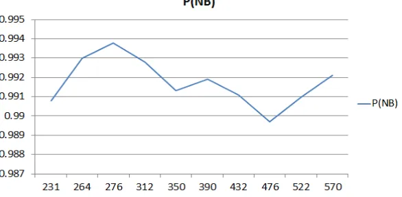
VI.RESULT AND DISCUSSION

In the fig 1, it shows the graph of length x theta VsPSNR for blind deblurring.

Fig 1:Length x theta Vs PSNR for bling deblurring

In the fig 2, it shows the graph of length x theta VsPSNR fornon blinddeblurring.

(7)

I

nternational

J

ournal of

A

dvanced

R

esearch in

E

lectrical,

E

lectronics and

I

nstrumentation

E

ngineering

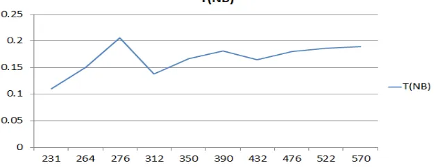
In the fig 3, it shows the graph of length x theta Vstime forblind deblurring.

Fig 3:Length x theta Vs time for bling deblurring

In the fig 4, it shows the graph of length x theta Vstime for non blinddeblurring.

Fig 4:Length x theta Vs time for non blingdeblurring

VII.CONCLUSION

(8)

I

nternational

J

ournal of

A

dvanced

R

esearch in

E

lectrical,

E

lectronics and

I

nstrumentation

E

ngineering

REFERENCES

[1] Mariana S. C. Almeida and M´ario A. T. Figueiredo, Fellow, ‘’Parameter Estimation for Blind and Non-Blind Deblurring Using Residual Whiteness Measures’’ IEEE TRANSACTIONS ON IMAGE PROCESSING, 2013 (TO APPEAR) 1

[2] M. Afonso, J. Bioucas-Dias, and M. Figueiredo, “Fast image recovery using variable splitting and constrained optimization,” IEEE Trans. Image Processing, vol. 19, pp. 2345–2356, 2010.

[3] M. S. C. Almeida and L. B. Almeida, “Blind deblurring of natural images,” in IEEE Int. Conf. Acoustics, Speech, and Signal Processing ICASSP, 2008, pp. 1261–1264.

[4] ——, “Blind and semi-blind deblurring of natural images,” IEEE Trans. Image Processing, vol. 19, pp. 36–52, 2010.

[5] M. S. C. Almeida and M. A. T. Figueiredo, “New stopping criteria for iterative blind image deblurring based on residual whiteness measures,” in Proceedings of the IEEE Statistical Signal Processing Workshop (SSP), pp. 337–340, 2011.

[6] B. Amizic, S. D. Babacan, R. Molina, and A. K. Katsaggelos, “Sparse Bayesian blind image deconvolution with parameter estimation,” in European Signal Processing Conference, 2010.

[7] S. D. Babacan, R. Molina, and A. K. Katsaggelos, “Variational Bayesian blind deconvolution using a total variation prior,” IEEE Trans. Image