Comparative Research on Robot Path Planning Based on GA-ACA and ACA-GA

(1)

University of Windsor University of Windsor

Scholarship at UWindsor

Electronic Theses and Dissertations Theses, Dissertations, and Major Papers

2017

Comparative Research on Robot Path Planning Based on GA-ACA

and ACA-GA

Chenhan Wang

University of Windsor

Follow this and additional works at: https://scholar.uwindsor.ca/etd

Recommended Citation Recommended Citation

Wang, Chenhan, "Comparative Research on Robot Path Planning Based on GA-ACA and ACA-GA" (2017). Electronic Theses and Dissertations. 7403.

https://scholar.uwindsor.ca/etd/7403

This online database contains the full-text of PhD dissertations and Masters’ theses of University of Windsor students from 1954 forward. These documents are made available for personal study and research purposes only, in accordance with the Canadian Copyright Act and the Creative Commons license—CC BY-NC-ND (Attribution, Non-Commercial, No Derivative Works). Under this license, works must always be attributed to the copyright holder (original author), cannot be used for any commercial purposes, and may not be altered. Any other use would require the permission of the copyright holder. Students may inquire about withdrawing their dissertation and/or thesis from this database. For additional inquiries, please contact the repository administrator via email

(2)

Comparative Research on Robot Path

Planning Based on GA-ACA and

ACA-GA

By

Chenhan Wang

A Thesis

Submitted to the Faculty of Graduate Studies through the School of Computer Science in Partial Fulfillment of the Requirements for

the Degree of Master of Science at the University of Windsor

Windsor, Ontario, Canada

2017

c

(3)

Comparative Research on Robot Path Planning Based on GA-ACA and ACA-GA

by

Chenhan Wang

APPROVED BY:

E. Abdel-Raheem

Department of Electrical and Computer Engineering

J. Chen

School of Computer Science

D. Wu, Advisor School of Computer Science

(4)

DECLARATION OF ORIGINALITY

I hereby certify that I am the sole author of this thesis and that no part of this

thesis has been published or submitted for publication.

I certify that, to the best of my knowledge, my thesis does not infringe upon

anyones copyright nor violate any proprietary rights and that any ideas, techniques,

quotations, or any other material from the work of other people included in my

thesis, published or otherwise, are fully acknowledged in accordance with the standard

referencing practices. Furthermore, to the extent that I have included copyrighted

material that surpasses the bounds of fair dealing within the meaning of the Canada

Copyright Act, I certify that I have obtained a written permission from the copyright

owner(s) to include such material(s) in my thesis and have included copies of such

copyright clearances to my appendix.

I declare that this is a true copy of my thesis, including any final revisions, as

approved by my thesis committee and the Graduate Studies office, and that this thesis

(5)

ABSTRACT

The path planning for mobile robots is one of the core contents in the field of

robotics research with complex, restrictive and nonlinear characteristics. It consists

of automatically determining a path from an initial position of the robot to its final

position. Due to classic approaches have several drawbacks, evolutionary methods

such as Ant Colony Optimization Algorithm (ACA) and Genetic Algorithm (GA) are

employed to solve the path planning efficiently.

Firstly, grid method is used to establish the environment model, and some

mod-ifications are made to accommodate ACA to path planning in a grid-based

environ-ment. Besides, genetic operators were introduced to the fundamental ACA (GA-ACA,

ACA-GA), using the crossover and mutation operators to expand the search space

and enhance the overall solution in the previous research work.

This thesis mainly introduces these two hybrid algorithms, GA-ACA and

ACA-GA, and will compare the performance of them under multiple grid maps in static

environments.

To verify the effectiveness of these two hybrid algorithms, a path planning

sim-ulation system for mobile robots is designed based on MATLAB development

envi-ronment. The experiment results show that the algorithm efficiency of GA-ACA and

ACA-GA is better than that of the traditional GA and ACA algorithms, and it is

more suitable to apply ACA-GA than GA-AGA regarding algorithms’ convergence

(6)

AKNOWLEDGEMENTS

I would like to express my sincere appreciation to my supervisor Dr. Dan Wu for

his constant guidance and encouragement during my whole Master’s period in the

University of Windsor. Without his valuable help, this thesis would not have been

possible.

I would also like to express my appreciation to my thesis committee members Dr.

Esam Abdel-Raheem, and Dr.Jessica Chen. Thank you all for your valuable guidance

and suggestions to this thesis.

Last but not least, I want to express my gratitude to my parents and my friends

(7)

TABLE OF CONTENTS

DECLARATION OF ORIGINALITY III

ABSTRACT IV

AKNOWLEDGEMENTS V

LIST OF TABLES VIII

LIST OF FIGURES IX

1 Introduction 1

1.1 Research Background . . . 1

1.2 Mobile Robots Path Planning . . . 2

1.2.1 Off-line Path Planning Algorithms . . . 2

1.2.2 On-line Path Planning Algorithms . . . 5

1.3 Thesis Motivation and Statement . . . 7

2 Review on Ant Colony Optimization 9 2.1 Introduction to Ant Colony Optimization . . . 9

2.2 Theroretical Explanation of ACO . . . 11

2.2.1 Combinatorial Optimization Problem . . . 11

2.2.2 Basis of ACO . . . 13

2.3 Main ACO Algorithm Implementations . . . 15

2.3.1 Ant System (AS) . . . 15

2.3.2 MAX-MIN Ant System (MMAS) . . . 16

2.3.3 Ant Colony System (ACS) . . . 17

2.4 Recent Researches about ACO . . . 18

2.4.1 Traveling Salesman Problem (TSP) . . . 18

2.4.2 Other Problems . . . 20

3 Robot Path Planning based on Ant Colony Optimization Algo-rithm 21 3.1 Modeling of Robot Motion Environment . . . 21

3.1.1 Robot Motion Environment division using the Grid Method . 22 3.1.2 The Description and Definition of Path Planning Problem . . 23

(8)

4 Robot Path Planning based on ACA integrating with Genetic

Al-gorithm (GA) 28

4.1 Genetic Algorithm and Robot Path Planning . . . 28

4.1.1 Introduction of Genetic Algorithm . . . 28

4.1.2 The Implementation Steps of GA on Robot Path Planning . . 29

4.2 Robot path planning based on GA-ACA . . . 33

4.2.1 Introduction of GA-ACA . . . 33

4.2.2 The Implementation Steps of GA-ACA on Robot Path Planning 33 4.3 Robot path planning based on ACA-GA . . . 35

4.3.1 Introduction of ACA-GA . . . 35

4.3.2 The Implementation Steps of ACA-GA on Robot Path Planning 36 4.4 Performance Evaluation Indexes of Ant Colony Optimization Algorithm 37 5 Simulation Experiments 39 5.1 Previous Experiments on GA-ACA and ACA-GA . . . 39

5.2 Simulation System . . . 40

5.3 Parameter Settings . . . 40

5.4 The Implementation of Simulation Experiments . . . 42

5.4.1 The First Group of Experiments . . . 42

5.4.2 The Second Group of Experiments . . . 48

5.4.3 The Thrid Group of Experiments . . . 50

5.4.4 The Fourth Group of Experiments . . . 55

6 Conclusion and Future Work 61

References 63

(9)

LIST OF TABLES

1 The simulation platform source code list . . . 40

2 The performance index of four algorithms in Experiment one . . . 47

3 The performance index of GA-ACA and ACA-GA in Experiment two 50

4 The performance index of GA-ACA and ACA-GA in Experiment three

under map 03 . . . 54

5 The performance index of GA-ACA and ACA-GA in Experiment three

under map 04 . . . 55

(10)

LIST OF FIGURES

1 Building Blocks of Mobile Robot Navigation. . . 2

2 Path Choosing based on Pheromone. (a) An example with real ants. (b) An example with artificial ants. . . 10

3 Example of Construction Graph in ACO. . . 12

4 Basis ACO Algorithm Framework. . . 13

5 The example of grid environmental map[10]. . . 23

6 The flow chart of genetic algorithm. . . 29

7 The example of path encoding. . . 30

8 The flow chart of GA-ACA. . . 35

9 The flow chart of ACA-GA. . . 37

10 The simulation system using MATLAB. . . 41

11 (a)The optimal path obtained by GA in map 01, the length of the optimal path is 14.4853; (b)The optimal path obtained by ACA in map 01, the length of the optimal path is 13.8995. . . 43

12 (a)The optimal path obtained by GA-ACA in map 01, the length of the optimal path is 13.8995; (b)The optimal path obtained by ACA-GA in map 01, the length of the optimal path is 13.8995. . . 43

13 (a)The optimal path length evolution graph by using GA in map 01; (b)The mean path length evolution graph by using GA in map 01. . 44

(11)

16 (a)The optimal path length evolution graph by using ACA-GA in map

01; (b)The mean path length evolution graph by using ACA-GA in

map 01. . . 45

17 The simulation result of ACA in map 01 . . . 46

18 (a)The optimal path obtained by GA-ACA in map 02, the length of the

optimal path is 14.4853; (b)The optimal path obtained by ACA-GA

map 02, the length of the optimal path is 14.4853. . . 49

19 (a)The optimal path length evolution graph by using GA-ACA in map

02; (b)The mean path length evolution graph by using GA-ACA in

map 02. . . 49

map 02. . . 50

map 03. . . 52

map 03. . . 53

(12)

map 04. . . 54

27 (a)The optimal path obtained by GA-ACA in map 05(6-96), the length

of the optimal path is 10.6569; (b)The optimal path obtained by

ACA-GA map 05(6-96), the length of the optimal path is 10.6569. . . 57

28 (a)The optimal path obtained by GA-ACA in map 05(41-70), the

length of the optimal path is 10.6569; (b)The optimal path obtained

by ACA-GA map 05(41-70), the length of the optimal path is 10.6569. 57

05(6-96); (b)The mean path length evolution graph by using GA-ACA

in map 05(6-96). . . 58

05(6-96); (b)The mean path length evolution graph by using ACA-GA

in map 05(6-96). . . 58

05(41-70); (b)The mean path length evolution graph by using GA-ACA

in map 05(41-70). . . 59

05(41-70); (b)The mean path length evolution graph by using ACA-GA

(13)

CHAPTER 1 Introduction

1.1 Research Background

With the development and maturation of computer technology, control theory,

ari-tifical intelligence theory and sensor technology, the research of robot has entered an

entirely new phase. Mobile robots, as an important branch of robotics, has received

wide recognition in an academic area all over the world.

A mobile robot is an automatic machine which has the capability to move around

in the environment [28]. Mobile robots can be “autonomous” which means they are

capable of navigating an uncontrolled environment without the need for physical or

electro-mechanical guidance devices.

From 1966-1972, the Stanford Research Institute was building and doing research

on Shakey the Robot [25], which was the first robot that can avoid obstacles

automat-ically. In 1999, Sony introduced AIBO [31], a robotic dog capable of seeing, walking

and interacting with its environment. In 2003, QRIO [16] was created by Sony to

follow up on the success of its AIBO entertainment robot. QRIO is the first humanoid

robot that can accomplish many actions such as running, jumping, throwing.

In recent years, mobile robots have become more commonplace in industrial,

agri-cultural and commercial settings. In all applications of mobile robots, they perform

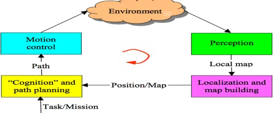
the navigation tasks using the following building blocks [26] in Fig.1. We can see that

navigation of a mobile robot involves perception of the environment, localization and

map building, cognition and path planning and motion control in Fig.1. Among the

(14)

1. INTRODUCTION

FIGURE 1: Building Blocks of Mobile Robot Navigation.

objective of path planning is about how to make mobile robots choose a collision-free

path according to the environment information.

1.2 Mobile Robots Path Planning

Path planning of a mobile robot is to determine a collision-free path from a start point

to a goal point optimizing a performance criterion such as distance, time or energy,

distance being the most commonly adopted criterion [26]. Based on the availability of

information about environment, there are two categories of path planning algorithms,

namely off-line and on-line. Off-line path planning of robots in environments where

complete information about stationary obstacles and trajectory of moving obstacles

are known in advance is also known as global path planning. When complete

infor-mation about environment is not available in advance, mobile robot gets inforinfor-mation

through sensors, as it moves through the environment. This is known as on-line

or local path planning. Both off-line and on-line path planning algorithms can be

categorized into classic approaches and evolutionary approaches.

1.2.1 Off-line Path Planning Algorithms

Examples of path planning in off-line environments are service robots operating

dur-ing maintenance period of a nuclear power plant, automated guided vehicles in a

(15)

1. INTRODUCTION

path planning algorithms can be categorized into classic approaches and evolutionary

approaches.

Classic Approaches

1. Configuration space approach [20]:

The central idea of configuration space approach is the representation of the

robot as a single point. Thus, the mobile robot path planning problem is

re-duced to a 2-dimensional problem. As robot is rere-duced to a point, each obstacle

is enlarged by the size of the robot to compensate. Then, we construct a

con-figuration space to describe the robot and its surroundings by using some basic

shapes such as a predefined convex polygon. The configuration space is

rep-resented as a connected graph, and then the path planning is performed by

searching the connected graph. This method is flexible, but the complexity of

this algorithm is proportional to the number of obstacles, and it can not

guar-antee that the method can output the shortest path under any circumstances.

That is one of the drawbacks of most classic approaches.

2. Visibility graph approach [20]:

The Visibility graph approach is drawn by joining two vertices of mutually

vis-ible polygonal obstacles that are present between start and target points. The

word ”Visibility” refers to the requirements of the robot between the vertices of

obstacles, the target point between the vertices of obstacles and the vertices of

one obstacle between the vertices of another obstacle can not cross the

obsta-cles. The shortest path is then identified through the roads obtained from the

visibility graph. Using some optimization algorithms can remove some

unneces-sary connecting lines to simplify the visibility graph, thus shortening the search

time. However, these optimization algorithms sometimes lacks flexibility, and

once the starting point and target point change, the visibility graph must be

reconstructed leading the low search efficiency.

(16)

1. INTRODUCTION

The cell decomposition approach computes the configuration space of the mobile

robot decomposes the resulting space into cells and then searches for a route

in the free space cell graph. Among the cell decomposition approaches, Grid

method [2] is the most popular one where grids are used to generate the map

of the environment. The main difficulty is how to find the size of the grids,

the lesser the size of grids, the more accurate will be the representation of

the environment. However, using lesser grids will result in exponential rise in

memory space and search range [14]. In my thesis, I will use the grid method

to establish robot motion environmental maps in chapter 3.

Evolutionary Approaches

Classic approaches sometimes take more time when selecting a feasible collision-free

path. Also, classic approaches tend to get locked in local optimal solution which may

be far inferior to the global optimal solutions. Moreover, path planning of a mobile

robot in the presence of multiple obstacles is found to be a non-deterministic

polyno-mial time hard (NP-hard) problem[3]. It becomes even more complicated when the

environment is dynamic. These drawbacks make the classic approaches incompetent

in complex environments. Hence, evolutionary approaches such as Genetic Algorithm

(GA), Particle Swarm Optimization (PSO), Ant Colony Optimization (ACO) and

Simulated Annealing (SA) is employed to solve the path planning problem efficiently.

1. Genetic Algorithm (GA):

GA is an optimization tool based on the mechanics of natural genetics and

selection. The first step in path planning using GA is a random generation

of the population containing alternative paths. [9] presented a visibility-based

repair approach that is used to quickly transform invalid paths into valid paths

and then subject to binary coded GA. GA with binary string is

computation-ally costly for the reason that before each evaluation of function, chromosomes

are transformed to phenotypes. [33] presented a genetic based path planning

(17)

1. INTRODUCTION

increases computation load resulting in higher execution time. The specific

process of how does GA works will be introduced in Chapter 4.

2. Particle Swarm Optimization (PSO) [17]:

Particle Swarm Optimization (PSO) is a widely used evolutionary algorithm in

path planning. It is an evolutionary computation technique inspired by social

behavior of bird flocking or fish schooling. Years of study on the dynamics

of bird and fish resulted in the possibilities of utilizing this behavior as an

optimization tool. Compared to GA, the advantages of PSO are that PSO is

easier to implement and there are fewer parameters to be adjusted.

3. Ant Colony Optimization (ACO) [4]:

ACO is inspired by the foraging behavior of ants for finding the shortest path

to the food source. The specific content about ACO and mobile robot path

planning based on ACO algorithm is introduced in Chapter 2 and 3.

4. Simulated Annealing (SA):

Simulated Annealing (SA) is a type of heuristic random search method and it

resembles the cooling process of molten metals through annealing. [21] present

a method employed SA for collision-free path amid static polygonal obstacles in

configuration space setting. [23] developed SA algorithm based approach which

used vertices of the static and dynamic obstacles as search space for dynamic

environments.

1.2.2 On-line Path Planning Algorithms

Applications of path planning in on-line environments include planet exploration,

mine industry, reconnaissance robots, etc [26]. Nowadays, evolutionary approaches

(18)

1. INTRODUCTION

Classic Approaches

1. Artificial Potential Field (APF) approach [18] :

The main idea of APF approach is that a point robot moves under the influence

of an APF in which obstacles are assumed to generate repulsive forces and the

target is assumed to generate attractive forces. The robot moves as per the

resultant of these forces. This approach is known for its mathematical elegance

and simplicity as path is found with very little computation. However, the

drawback of this approach is that robot may become stagnant or trapped when

there is a cancellation of equal magnitudes of attractive and repulsive forces.

2. Vector Field Histogram approach [1]:

The central idea of this approach is that a polar histogram is generated to

represent the polar density of obstacles around a robot at every instant. The

robots steering direction is chosen based on the least polar density and closeness

to the goal. In a given environment, the polar histogram must be regularly

regenerated for every instant and hence the method is suited for environments

with sparse moving obstacles.

3. Velocity obstacle approach [11]:

This method consists of choosing avoidance maneuvers to avoid static and

mov-ing obstacles in the velocity space. They used basic heuristic strategy for

priori-tizing objectives such as averting collisions, attaining the goal or accomplishing

trajectories with preferred topologies.

4. Dynamic windows approach [12]:

The dynamic window approach contains the feasible linear and angular

veloci-ties taking into consideration acceleration capability of robot. Then the velocity

at the next instant is optimized for obstacle avoidance, subject to vehicle

(19)

1. INTRODUCTION

Evolutionary Approaches

When applying on-line path planning algorithms, computation time is the most

im-portant aspect that we should consider. However, with classic approaches, the results

can hardly be achieved in very quick time because of incomplete information of the

environments.Therefore, classic approaches are often combined with evolutionary

ap-proaches like GA, PSO, etc. to overcome their drawbacks.

1. Evolutionary APF [30]:

The evolutionary APF algorithm is to derive optimal potential field functions

using GA. When the robot is trapped, a separate algorithm named escape-force

is introduced to recover from a trap.

2. APF combined with SA [22]:

This approach considers the problems of goal non-reachable with obstacles

nearby (GNRON) and local minima in soccer robots. New potential functions

have been derived by considering the distance information of start and target

points for GNRON problem.

1.3 Thesis Motivation and Statement

The thesis is mainly focused on robot path planning problem based on ant colony

optimization algorithm and two ant colony algorithms combined with genetic

algo-rithms, namely GA-ACA and ACA-GA. The previous research work of [15] and [35]

indicated that GA-ACA and ACA-GA perform better than the traditional algorithm,

ACA. However, the researchers had not compared the performance of GA-ACA and

ACA-GA in the previous work. This motivates me to do the further study on these

two algorithms.

Chapter 2 introduces the concept of ant colony optimization algorithm (ACA)

and describes how it is inspired by the nature phenomenon. Then, we give detailed

explanation of ACA in theory and describe three main ACA algorithms: Ant System,

(20)

1. INTRODUCTION

related to ACA and how it applies to the NP-hard problems.

Chapter 3 establishes the robot motion environmental model by using grid method

and introduces two main methods for grid making. Then, we describe how ant colony

optimization algorithm (ACA) for robot path planning works under grid

environmen-tal maps.

In chapter 4, two algorithms based on the ant colony algorithm are proposed:

GA-ACA algorithm and ACA-GA algorithm. We describe the process of GA-ACA

and ACA-GA respectively and compare the differences between these two hybrid

algorithms.

In chapter 5, based on MATLAB platform, we design four comparative

experi-ments to verify the validity and effectiveness of the GA-ACA and ACA-GA algorithm

under different grid maps.

The chapter 6 summarizes the work of this thesis and points out the limitations of

(21)

CHAPTER 2 Review on Ant Colony

Optimization

2.1 Introduction to Ant Colony Optimization

Ant Colony Optimization (ACO) was first introduced and proposed by Marco Dorigo

in his Ph.D. thesis in 1992 [4]. It is a metaheuristic that inspired by the food seeking

behavior of ant colony. As we all know, in the natural world, the ant is a kind of

social insect. Although the behavior of a single ant looks quite simple, multiple ants

can cooperate to construct a huge social group to accomplish much more complicated

tasks. When the ants search for food, initially they just wander randomly to explore

the area near their nest, and different ants can choose different paths to explore due

to their random behavior manner. As soon as one of the ants successfully locate the

food source, this ant will carry bearable amount of food back to its nest. During their

return journey, assuming that the ants remember its traveled route from the nest to

the located food source, it will return to the nest along the same route, and leave

chemical pheromone trail on the ground. The amount of the pheromone left may vary

depending on the quality and quantity of the food. Then, other ants now can choose

the route that has denser pheromone (which can be treated as a better route) and

guides them to the food source. This behavior will also cause the originally better

route becomes even much better by aggregating more pheromones.

This ant colony behavior can be modeled as metaheuristic, which is the core

(22)

2. REVIEW ON ANT COLONY OPTIMIZATION

(a) (b)

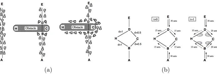
FIGURE 2: Path Choosing based on Pheromone. (a) An example with real ants. (b) An example with artificial ants.

algorithms that are used to obtain good enough solutions to solve hard combinatorial

optimization problems (CO). The goal of CO problem is to find out a good enough

solution in a reasonable amount of time.

Considering the scenario introduced in [8] as shown in Fig.2 (a), there is a path

between food source E and nest A. When an obstacle is placed to cut off the path,

ants have to decide whether to turn left or right (position H or C). Firstly there are no

pheromones left at path BH, BC, DH and DC , which can be clearly seen in Fig.2 (b);

thus the probability of choosing left or right is equal. However, since BCD is shorter

than BHD, the ants turned to C will arrive E faster than the ants which turned to H.

When the first ant returned from E arrives D, the path DC have more pheromones

since more ants have passed D from C than from H, so that this first ant that has

finished the trip will have higher probability of choosing path DCB. The consequence

is that the pheromone on the shorter path will grow faster than on the longer path,

and therefore the probability of choosing paths is quickly biased towards the shorter

one.

Having the conclusion we draw in the above paragraph, now considering the

ab-stract model shown in Fig.2(b), 30 ants depart in 1 time slot, the length of BH and

HD are both 1, and the length of BC and CD are both 0.5, if we neglect the length

of AB and DE, the length of ABHDE (path L) is 2 times larger than ABCDE (path

(23)

ants depart at t= 1, the probability of choosing path R is 2 3.

2.2 Theroretical Explanation of ACO

Ant Colony Optimization (ACO) algorithms can be treated as stochastic search

pro-cedures. Although multiple ACO algorithms exist, the central component of these

algorithms is the pheromone model that is used to sample the search space[6]

proba-bilistically. The model of Combinatorial Optimization (CO) problem can be used to

implement the pheromone model. In the following subsection, we will first introduce

the model of solving CO problem.

2.2.1 Combinatorial Optimization Problem

[6], [5] mentioned that a CO problem could be defined as: P = (S,Ω, f), where

• Sis a finite solution set; it is defined over a finite set of discrete decision variables

Xi, (i= 1,2, ..., n);

• Ω represents a set of constraints among the discrete decision variables Xi; • f is an objective function that assigns a cost value to every solution. f can be

defined as f :S →_R+_.

For the solution setS , which can also be called search space, the discrete decision variable Xi are assigned with domain values vji, where v

j

i ∈ Di = {v1i, vi2, ..., v

|Di|

i }.

s∈ S is called a feasible solution when s is a complete assignment that each discrete decision variables Xi has a domain value assigned that satisfies the constriant set Ω.

Moreover, a feasible solution s∈ S is called a globally optimal solution only if for all

s∗ ∈ S,f(s∗)≤f(s). Sometimes there is not only one globally optimal solution, the set of globally optimal solutions can be represented as S∗ _{⊆ S}_.

This CO problem model is a finite set of solution components and a pheromone

model. The discrete decision variable Xi and one of its domain valuesv j

i is asolution

(24)

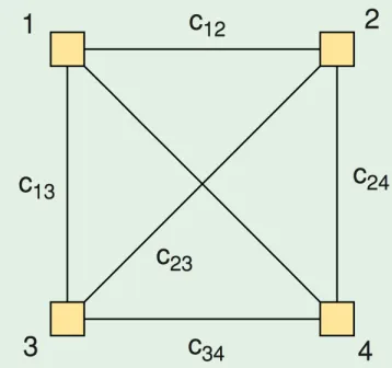
FIGURE 3: Example of Construction Graph in ACO.

model, each of the solution component cj_i has a pheromone trail parameter τ_ij. All pheromone trail parameters are denoted byτ. We use Cto represent all the solution components, which means C={cj₁, cj₂, ..., cj_n}.

The following is a specific example of the described CO problem. As shown in

Fig.3, in ACO problems, an artificial ant builds a solution by traversing the fully

connected construction graph denoted by GC = (V, E), V is the set of vertices, E is

the set of edges. In our simple example, the construction graph contains four vertices,

artificial ants move from vertex to vertex along the connected edges. For the solution

components C we just mentioned, in this case, there are four solution components:

cj_i, (i= 1,2,3,4), which can map to the four discrete variablesXi, (i= 1,2,3,4), and

also can represent the four vertices of the construction graph. For example, a solution

component cj₂ can represent node 2 in the construction graph, and X2 indicates the

node to be visited after node 2, soX2 =cj2 means the next node visited is nodej, the

value range ofj is|Di|, which can be treated as the connected vertices withi. And in

general,cj_i indicates a solution that node j should be visited immediately after node

i, in order words, it indicates edge (i, j), ants deposit pheromoneτ_ij on the edges (i, j) describes its importance of reaching the best- optimized solution. The way how an

artificial ant builds a solution by traversing the fully connected construction graph

(25)

FIGURE 4: Basis ACO Algorithm Framework.

2.2.2 Basis of ACO

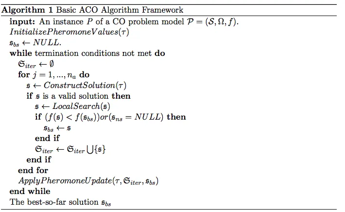
Fig.4 shows the framework of basic ACO algorithm [6]. Initially, all pheromone values

τ_ij that belongs to the set of τ (the pheromone model) are initialized to a constant valuec >0, this process is finished by the functionInitializePheromoneValues shown in Algorithm 1. We assume there arenaartificial ants in total. During each iteration,

naants use the current pheromone model to probabilistically construct solutions to the

CO problem. For each ant, the function ConstructSolution is executed to construct

a solution component. This function is also the basic building block component of

any ACO algorithm as it is a constructive heuristic for probabilistically constructing

solutions. The solution constructing process can be reflected as selecting sequences of

elements from the finite set of solution componentsC, since the solution is constructed

by each ant in each iteration, thus we call this as partial solution, usingsp to represent it. The construction process is described as follows:

• Start with the empty partial solution set sp =∅;

(26)

com-2. REVIEW ON ANT COLONY OPTIMIZATION

ponent is in the set C but not yet included in the set sp.

This process can be visualized as a continuous walk along the edges of the

construc-tion graph GC = (V, E), all the vertices can be treated as the solution components

in the set C as we described in the previous section. In each step of the solution

construction, thecj_i that belongs tosp _{is chosen probabilistically based on the current}

pheromone model. The probability of choosing a specific solution component cj_i is proportional to [τ_ij]α _·_[_η₍_cj

i)]β[6]. η is a function that assigns to each feasible

solu-tion component, which can be treated as a heuristic value or heuristic informasolu-tion.

Parametersα and β are all positive numbers that determine the relative importance of pheromone value and heuristic information. [6] also mentioned the heuristic

in-formation is optional, but if included, the ACO algorithm can usually achieve better

performance. If considering the heuristic information, the probability of choosing the

next solution component cj_i is defined as follows:

P(cj_i|sp) = [τ

j

i]α·[η(c j i)]β

P

ck i∈sp[τ

k

i]α·[η(cki)]β

(1)

This equation is also called transition probabilities, which is first used in [8]. Each

possible solution component cj_i is expressed as the weight of pheromone level and weight of heuristic information (total weight of cj_i). Therefore, the probability of choosing cj_i is the weight proportion of cj_i among the total of ck

i with all possible

values of k.

In algorithm 1, the LocalSearch function is an optional step. It is used to

im-prove the solutions obtained by an individual ant after the partial solution has been

constructed and before updating the pheromone. As mentioned in [5], LocalSearch is

usually included in state-of-the-art ACO algorithms.

After all the ants finished the partial solution construction in one iteration, the

pheromone should be updated to increase its value to keep strong association with

the good or promising solutions. There are two main steps:

(27)

Usually, most ACO algorithms use the following pheromone update rule:

τ_ij ←(1−ρ)·τ_ij+ ρ

S_upd ·

X

{s∈Supd|cji∈s}

F(s) ₍₂₎

In the equation, i = 1,2, ..., n and j ∈ |Di| , |Di| represents all the connected

vertices with i (have accessible paths to i). The parameterρ is an evaporation rate, with each update of the pheromone, the percentage of ρ of former pheromone will be deleted. The pheromone evaporation can avoid ACO algorithm converging too

quickly. Supd is the subset ofSiter, and SiterSsbs contains all the sp created by each

ant in the current iteration. sbs represents the best-so-far solution. F(s) is usually

called a quality function.

2.3 Main ACO Algorithm Implementations

During the past several decades, lots of different ACO algorithms have been proposed,

based on our knowledge, there are three kinds of main ACO algorithm

implementa-tions: Ant System (AS), MAX-MIN Ant System (MMAS), Ant Colony System (ACS).

We will give detailed explanations about these three main ACO algorithms.

2.3.1 Ant System (AS)

Ant System (AS) is the first proposed ACO algorithm in the world[8], and has been

successfully applied into the famous Traveling Salesman Problem. Similar with the

basis of ACO we introduced in section 2.2, AS updates pheromone in each iteration

based on the solution set constructed by all the ants in each iteration. By visualizing

AS as a connected construction graph (refer to Fig.3), for a vertex pair (i, j) and edge (i, j), we can re-define the pheromone τ_ij as follows:

τ_ij ←(1−ρ)·τ_ij +

na

X

k=1

∆τ_ijk (3)

∆τ_ijk =      Q Lk

if antk used edge (i, j) as part of its path

0 otherwise

(28)

pk_ij =         

τ_ijα·ηβ_ij P

cil∈N(sp)τ

α il ·η

β il

ifcij ∈N(sp)

0 otherwise

(5)

In the equation (3), ρ is the evaporation rate, na is the total number of artificial

ants, ∆τ_ijk is the quantity of pheromone left on edge (i, j) by ant k. Equation (4) gives the detail of how to calculate ∆τk

ij. Qis a constant, andLkis the total length of

all the edges that traveled by ant k in the current iteration. By having the τ_ij value, the probability for ant k to go to vertex j from i is calculated as shown in equation (5). N(sp) is the set of feasible solution components that haven’t been added into the solution set yet, if visualized as graph, it can be treated as the unvisited edges by

ant k. The heuristic information ηij =

1

dij

, where dij is the length of edge (i, j).

Therefore, similar to the process we introduced in Section 2.2, in each iteration,

based on the paths traveled by each ant, the pheromone τij on each edge of the

connected construction graph is updated using equation (3). Then based on the

updated pheromone, next round iteration begins, ants will travel through the graph

again probabilistically choosing next vertex by using equation (5).

Based on the concept of AS, the authors also proposed an algorithm called

ant-cycle to apply to the famous Travelling Salesman Problem (TSP). In their proposed

algorithm, they set a terminating threshold N Cmax to terminate the iteration at last

to get the final optimal solution set.

2.3.2 MAX-MIN Ant System (MMAS)

MAX-MIN Ant System is proposed in the year 2000 [29], which is an improved ACO

algorithm based on the original AS. MMAS differs from AS mainly in the following

three aspects.

• After one iteration, only one single ant updates pheromone τ. This ant is the one who found the best solution in the current iteration (iteration-best ant) or

(29)

• The range of possible pheromone values on each solution component is limited to an interval [τmin, τmax];

• Initialize the pheromone values toτmax.

Based on the first different point listed above, the equation for updating pheromone

τij is modified as follows:

τij ←(1−ρ)·τij+ na

X

k=1

∆τ_ijbest (6)

By setting the range of [τmin, τmax], if the updated τij is greater than τmax, then

the value should be set to τmax. Also, if the updated τij is smaller than τmin, the

value should be set to τmin. And ∆τijbest is decided by

1

Lbest

, if edge (i, j) belongs to the path at the current iteration.

The author of MMAS claims that the main contribution they made is to utilize the

pheromone limits to prevent premature convergence. Using the range of [τmin, τmax]

can prevent some edges have too large pheromone value, which can cause the solution

convergence too soon so that the final solution may not be the best global solution.

Not only MMAS, but also some other improved ACO algorithms also utilize the idea

of only updating the pheromone by the single ant which found the best solution in

current single iteration.

2.3.3 Ant Colony System (ACS)

The Ant Colony System (ACS) was first proposed in 1996 [13], it is also proposed by

the same author (the author that proposed the concept of Ant Colony Optimization

in his Ph.D. thesis at 1992. [4]). The proposed ACS algorithm has 4 phases:

• Phase 1: initialize the pheromone value to τ0, place each artificial ant k based

on some pre-defined policies to different vertices of the construction graph;

• Phase 2: execute in a cycle, in each round of the cycle, an artificial antk makes a move from vertex i to vertex j and update the τij based on the following

formula:

(30)

• Phase 3: the artificial ants which achieved the pathLbest computes the delayed

reinforcements (Lbest−iter)

−1

, and updatingτij as follows:

τij ←(1−α)·τ_ij +α·(Lbest−iter)−1 (8)

• Phase 4: check whether the termination condition is satisfied, if not, jump back to Phase 2.

As we can see in the 4 phases of the ACS algorithm, the main difference between

AS and ACS is that ACS updates the pheromone value τij for the edge (i, j) in each

move (each construction step) of the artificial ants (move from one vertex to another

vertex), not like AS, only updates τij at the end of one construction process after

one iteration was done (all the artificial ants finished their visiting to all vertices).

We call the updates in each construction step as local pheromone update, and the

updates after one iteration is called offline pheromone update. The main goal of the

local update is to diversify the search performed by subsequent ants inside the current

iteration. It can be used to decrease the pheromone concentration on some specific

traversed edges so that the probability of several ants create identical paths during

one iteration is lower.

2.4 Recent Researches about ACO

Since the year 1992 when Macro Dorigo proposed the first concept of ACO, the

interest of digging into ACO problem has risen gradually. ACO has been applied

into the full range of different research topics. In the following subsections, we will

introduce some current research branches utilizing ACO.

2.4.1 Traveling Salesman Problem (TSP)

The majority of the applications of ACO is to solve NP-hard problems. The

defi-nition of NP-hard problem is the best-known algorithms to solve the problem have

(31)

ap-2. REVIEW ON ANT COLONY OPTIMIZATION

from traditional algorithms to solve the NP-hard problem. ACO can quickly work

out high-quality good enough solutions.

Traveling Salesman Problem (TSP)is one of the most famous NP-hard

prob-lems, and it is also the most common problem been studied by most of the ACO

researchers over the years. Firstly, [8] described using Ant System (AS) to solve TSP;

later, [13], [7], [7] mentioned using Ant Colony System(ACS) to solve TSP. TSP can

be defined as follows:

Given a list of cities and distances between each pair of cities, find the shortest

route that travels to each given cities and finally returns back to the original city.

It is a typical combinatorial optimization problem. We can refer to Fig. 3, each

vertices in the construction graph can be treated as a city; the weighted edges can be

treated as the distances between cities. If using ACS to solve TSP, the four phases

listed in section 3.3 should be followed. For the Combinatorial Optimization Problem

P = (S,Ω, f), Xi ∈ S represent the cities in the graph, the solution component cji

means choosing the path from city i to city j. Also, the pheromone valueτij means

the level of pheromone information left on the path from city i to city j. And the probability of choosing next vertex for an artificial ant is computing using equation

(5) and the pheromone value is updated using equation (7), (8) if using ACS, or

equation (3), (4) if using AS.

In [7], the authors compared the performance of ACS with other naturally

in-spired global optimization methods including simulated annealing (SA), evolutionary

program- ming (EP), genetic algorithm (GA), etc. Their comparison results are

shown in Fig. 3. They reported the best integer tour length (path length when

fin-ished traveled all cities and back to the original city), the best real tour length in

parentheses, and number of tours / iterations required to find the best integer tour

length in square brackets. We can see for the number of iterations, ACS significantly

(32)

2.4.2

CHAPTER 3 Robot Path Planning based on Ant

Colony Optimization Algorithm

3.1 Modeling of Robot Motion Environment

The establishment of robot motion environmental model is a very important part

of robot path planning. The actual working environment of the robot is a realistic

physical space, however, the space that robot path planning algorithm to deal with

is an abstract environmental space. Environmental modeling is one mapping from

physical space to abstract space.

This section uses the grid method to establish the environmental model in order

to simulate the actual working space of the robot. Using grids to represent maps of

the robot working space can avoid complex calculations when dealing with obstacle

boundaries. In the application of grid method, the division of the grid size is critical:

the smaller of the grid size, the more accurate the representation of the obstacles,

but at the same time, a huge amount of storage is required and the search range of

the algorithm will increase exponentially; However, the larger of the grid size, the

(34)

3. ROBOT PATH PLANNING BASED ON ANT COLONY OPTIMIZATION ALGORITHM

3.1.1 Robot Motion Environment division using the Grid

Method

For any shape of two-dimensional topographic, there are always limited number of

obstacles, the coordinate location of these obstructions are easily mapped, so these

can be regarded as known environmental information. Grid map can be established

after traverse learning of two-dimensional space.

Without regard to robot information in height direction, two-dimensional space

robots work is marked as AS, whose inner distributes limited static obstacles [35]. The size and location of the obstacles have been known, and they will not change

in the motion process. In AS, the left bottom in Fig.5 is regarded as coordinates origin, the level right as X axis positive direction, the vertical upward as Y axis positive direction to establish Cartesian coordinate system P

, respectively, and the

maximum of the X axis and Y axis are Xmax and Ymax.

Take the walk step length of the robot is δ. The step δ is used to divide X axis and Y axis regularly to get grids respectively. The number of grids in each line is

Nx = Xmax/δ, and the number of grids in each row is Ny = Ymax/δ. If there is no

obstacle in a grid, this grid will be called free grid and filled with white, or it will be

called obstacles grid and filled with grey.

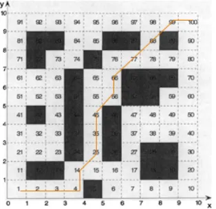
When Xmax is equal to Ymax (both are equal to 10), and δ is 1, the grid model of

the robot work space is shown in Fig.5.

We adopt two main methods for grid making, named Rectangular coordinate

method and Serial number method.

• Serial number method: From the left bottom of the grid map, coding the grid from bottom to top, from left to right in Fig.5. The serial number is from 1 to

100. The grid using serial number method to mark is gn, e.g., the grid of serial

number 1 is marked as g1.

(35)

FIGURE 5: The example of grid environmental map[10].

There is a conversion relation between serial number si(i= 1,2,3, ...,100) and its

coordinates: _

 

 

xi=mod(si−1,10) + 0.5

yi =int((si−1)/10) + 0.5

(1)

,wheremodrepresents remainder operation andintrepresents rounding operation. In my thesis, we define the starting point of robot path planning as g1 in the left

bottom of the map, likewise, the target point of robot path planning as g100.

3.1.2 The Description and Definition of Path Planning

Prob-lem

To simulate the real ant colony seeking food behavior, we assume that the starting

point of robot path planning g1 as ant colony nest, and the target point gn as food

source. Robot path planning based on ant colony optimization algorithm is actually

(36)

mutual effect and cooperation to avoid all obstacles. We make several definitions to

explain the following sections conveniently.

• Definition 1: city = 1,2, ..., nrepresents the set of all grids,nis the total amount of girds, n= 100 in Fig.5;

• Definition 2: ant = 1,2, ..., m represents the set of all ants, m = 10 in this algorithm of my thesis;

• Definition 3: DIST AN CEn∗n is a matrix that records the distance between

each grid. DIST AN CE(i, j) represents the distance between gi and gj, we

have this equation:

DIST AN CE(i, j) = q

[a(i)−a(j)]2+ [b(i)−b(j)]2 (2)

,a(i) anda(j) are the X-axis of theg(i) andg(j) respectively, likewise,b(i) and

b(j) are the Y-axis of the g(i) and g(j) respectively.

3.2 Robot Path Planning based on Ant Colony

Optimization Algorithm (ACA)

3.2.1 Several Changes of ACA when Solving Robot Path

Planning

The mathematical model of ACA has solved the TSP problem successfully. Before

ap-plying ACA on the field of robot path planning, we should make several modifications

on ACA based on the features of robot path planning.

Using Pseudo-random-proportional Rule instead of Random-proportional

Rule to Choose Path

In Ant System introduced in section 2.3, we have the following state transition rule,

(37)

which ant k in cityi chooses to move to the city j.

pk_ij =         

τ_ijα·ηβ_ij P

cil∈N(sp)τ

α il ·η

β il

ifcij ∈N(sp)

0 otherwise

(3)

Obviously, the ant choose the next path relied heavily on probability under

random-proportional rule. To make the most of the heuristic information between adjacent

nodes and pheromone value existed on each path, we decide to use a new state

transi-tion rule called pseudo-random-proportransi-tional rule, given by (4), instead of the previous

random-proportional rule. s=     

argmax{τ_ilα·η_ilβ} ifq≤q0 (exploitation)

S otherwise (biased exploration)

(4)

, where q is a random number distributed in [0,1],q0 is a parameter, 0≤q0 ≤1,

and S is a random variable selected according to the probability distribution given in (3). The parameter q0 determines the relative importance of exploitation versus

exploration: every time an ant in city i has to choose a city j to move to, it samples a random number q. If q ≤ q0, then the best edge, according to (4), is chosen

(exploitation), otherwise an edge is chosen according to (3) (biased exploration).

Redefine of Heuristic Information ηij

In Ant System (AS), ηij =

1

dij

, and dij is the distance between grid gi and grid gj.

However, in the robot motion environment introduced in this thesis,dij could be 1 or √

2 so that the function of heuristic search is not obvious and has few differences. To

increase the probability of ants choosing the next grid that closer to the destination

grid gn, we redefine the heuristic information, given by (5):

ηij =

C djn

(5)

, whereCis a constant anddjnis the distance between next gridgj and the destination

(38)

3.2.2 The Implementation Steps of ACA on Robot Path

Plan-ning

Under grid map environment which has n grids, The implementation steps of ACA on Robot Path Planning are shown as follows:

Step 1: Set the initial parameters, initialize ant colony

The parameters including start gridg1, destination gridgn, iteration timesNc = 0,

max iteration timesNc max, impact index of pheromonesα, impact index of heuristic

factor β, pheromone evaporation rateρ, constant Q, and initial pheromone τij(0) =

const.

Set routh bestto record the shortest path in every iteration, length bestto record the length of the shortest path in every iteration,length averageto record the average length of all paths got in each iteration.

All the ants m are placed in the start grid g1, and put g1 into the taboo table of

the ant k, tabuk(k = 1,2,3, ...m) ;

Step 2: Each ant move into next grid

According to pseudo-random-proportional rule given by (3) and (4), each ant

selects a next grid to move in, and the next grid will put into the taboo table of this

ant. If the current grid is the destination grid, let this ant dead.

Step 3: Repeat step 2, until all the ants have selected the next grid

Step 4: Local pheromone update

After all ants have selected the next grid, the algorithm implements local pheromone

updating given by (6).

τij(n+ 1) = (1−ρ)·τij(n) +ρ·∆τijk (6)

, where ∆τk

ij is a constant,τmin <∆τijk < τmax. Whenτij(n+1)< τmin, setτij(n+1) =

τmin; When τij(n+ 1) > τmax, set τij(n+ 1) =τmax

Step 5: Repeat Step 2, Step 3, and Step 4, until all the ant move into

the destination grid

(39)

Step 7: Global pheromone update

After each iteration, the algorithm implements global pheromone updating given

by (7) and (8).

τ(r, s)←(1−α)τ(r, s) +α∆τ(r, s) (7)

∆τ(r, s) =   

 

1 Lbest−iter

if (r,s) belongs to the global optimal path

0 otherwise

(8)

Step 8:Clear the tabuk, Nc = Nc + 1, if Nc ≤ Nc max, move to Step 2; if

Nc ≤ Nc max, move out the whole iteration, get the optimal path and the

(40)

CHAPTER 4 Robot Path Planning based on

ACA integrating with Genetic

Algorithm (GA)

4.1 Genetic Algorithm and Robot Path Planning

4.1.1 Introduction of Genetic Algorithm

Genetic Algorithms became popular through the work of John Holland in the early

1970s. A Genetic Algorithm (GA) is a meta-heuristic inspired by the process of

natural selection that belongs to evolutionary algorithms (EA) [24].

In a genetic algorithm, an optimization problem can be simplified to a process

to find a better solution from a population of candidate solutions. Each candidate

solution has a set of properties which can be mutated and altered; traditionally,

solutions are represented in binary as strings of 0s and 1s, but other encodings are

also possible.

A typical genetic algorithm requires a genetic representation of the solution

do-main and a fitness function to evaluate the solution dodo-main. A standard

representa-tion of each candidate solurepresenta-tion is as an array of bits. The main property that makes

these genetic representations convenient is that their parts are easily aligned due to

their fixed size, which facilitates simple crossover operations [34]. Variable length

(41)

4. ROBOT PATH PLANNING BASED ON ACA INTEGRATING WITH GENETIC ALGORITHM (GA)

FIGURE 6: The flow chart of genetic algorithm.

this case. Once the genetic representation and the fitness function are defined, a

GA proceeds to initialize a population of solutions and then to improve it through

repetitive application of the mutation, crossover, inversion and selection operators.

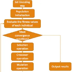
In summary, the core content of genetic algorithm involves the generation of

ini-tial population, the selection of fitness function, the design of genetic operators and

termination conditions. The flow chart of GA is shown in Fig.6.

4.1.2 The Implementation Steps of GA on Robot Path

Plan-ning

Due to the capability of rapid global search and rapid search to global optimal path

that genetic algorithms have, genetic algorithms have been applied to multi-robot

path planning. In this section, it will adopt genetic algorithm to find the optimal

path based on the grid environmental map introduced in chapter three. The

imple-mentation steps of GA on Robot Path Planning are shown as follows:

(42)

FIGURE 7: The example of path encoding.

Binary coding or floating point coding is not suitable when using GA to solve

robot path planning problems. This thesis adopts a series of grid numbers as path

encoding, which means each path can be represented as a series of numbers. Due to

one path can not pass the obstacle grids, nor can it pass through the repeated grids,

this series of numbers can not be the serial number of obstacle girds or repeated girds.

For example, one path can be represented as follows in Fig.7:

1-2-3-4-14-25-35-45-56-66-77-88-99-100

The path is identified with orange line, and the figure 1 represents the serial

number of path planning’s starting grid, likewise, the figure 100 represents the serial

number of path planning’s target grid. The rest of numbers represent the serial

number of path planning’s middle grids.

Step 2: The generation of initial population

In the grid environment model, the path from the starting grid to the target grid

is variable, so in the genetic algorithm, the chromosome representing the path is also

variable. The initial path individual generation process is as follows: starting from

the starting grid 1, step by step, non-repeated to choose next free grid until moves

to the target grid 100. Therefore, the path population consist of the multiple path

individuals that gained from step 2.

Step 3: The selection of fitness function

(43)

stability of the genetic algorithm. As robot path planning problem has to satisfy

the condition of the shortest path, the fitness function set the path length as the

evaluation criterion. The fitness function in this thesis is shown as follows [35]:

f = 1

(1 +√ 1

N−1)d

(1)

where,N represents the number of passed grids in each path,drepresents the length of each path.

Step 4: The design of genetic operators

This thesis introduces four genetic operators: selection operator, crossover

opera-tor, mutation operaopera-tor, deletion operator.

• Seletion operator:

The selection operation is also called copy operation, which means it selects the

individual from the parent and passes individual to the offspring instantly. In

the process of copy, the probability that an individual in each parent copied to

the next generation is determined by the value of its fitness function. Individuals

with larger fitness function value, ie, individuals with shorter paths, are more

likely to be copied to the next generation. So how to select individuals to

copy to the next generation; this thesis uses roulette method. To illustrate the

working principle of roulette method, assuming that the population has path

1, path 2 and path 3 three individuals, with the fitness function value 2, 3, 5,

respectively. The probability of these three individuals to be selected is [0.2,

0.3, 0.5], and cumulative probability is [0.2, 0.5, 1]. Generate a random number

rand between 0 to 1, if rand falls in [0, 0.2], path 1 is selected; if rand falls in [0.2, 0.5], path 2 is selected; if rand falls in [0.5, 1], path 3 is selected.

• Crossover operator:

The crossover operation is to intersect different individuals from the parent

to produce new individuals. The typical crossover methods have single point

crossover, double point cross and multipoint crossover. This thesis uses single

(44)

two path individuals from the parent to cross and exchange the part of the path

afer the intersection point.

For example, One path is: 1-4-14-25-45-56-66-99-100, another path is

1-4-14-15-65-66-76-80-100, the crossover grid is 66, then two path will be

1-4-14-25-45-56-66-76-80-100 and 1-4-14-15-65-66-99-100, respectively.

• Mutation operator:

Mutation operation plays a key role in increasing population diversity.

Con-sidering the diversity of the paths after searching, the path individuals after

mutation operation is not considered to be superior to the path individuals

be-fore mutation operation. According to a given mutation probability, we select

a serial number of grid from one path individual randomly and replace an

ar-bitrary serial number with the selected serial number of the grid. For example,

one path is 1-4-14-25-45-56-66-99-100, if the mutation grid is 56, if we choose

55 to replace that grid, the new path after mutation will be

1-4-14-25-45-55-66-99-100,

• Deletion operator:

Due to the initial randomness and mutation operations, the individuals from

the path population may have an obstacle grid number, and the path individual

can not contain an obstacle grid number, which requires the removal of obstacles

in the path individual. When implementing crossover and mutation operations,

the path individuals may contain some repeated grid numbers, which is not

allowed, It is necessary to delete the serial numbers of which two repeated grids

(45)

4.2 Robot path planning based on GA-ACA

4.2.1 Introduction of GA-ACA

Genetic algorithm (GA) is a global optimal algorithm based on natural selection

and natural genetic, with the capability of rapid global search and rapid search to

global optimal path. However, without the use of the feedback information of the

sys-tem, this method usually cause redundancy iteration and reduce solution efficiency.

Ant colony optimization algorithm (ACA) converge to the optimal path through

pheromone accumulation and update, with distributivity, parallelism and global

con-vergence ability, but in the initial stage pheromone among all paths are equal, which

makes it equate to greedy algorithm and leads to slow convergence speed, the obtained

solution is often not the optimal solution.

To overcome the drawback of two algorithms in robot path planning application,

a method of path planning was put forward, which combined genetic algorithm with

ant colony optimization algorithm, called GA-ACA. GA-ACA algorithm is firstly

using genetic algorithm to generate distributed initialization pheromone, then using

ant colony algorithm for the optimal solution, thus this way effectively combines fast

convergence of genetic algorithm and information positive feedback mechanism of ant

colony algorithm.

GA-ACA is superior to the genetic algorithm in computational efficiency, and is

superior to the ant colony optimization algorithm in time efficiency.This algorithm

has become a kind of heuristic algorithm which has better computational efficiency

and time efficiency.

4.2.2 The Implementation Steps of GA-ACA on Robot Path

Planning

Under grid map environment which has n grids, The implementation steps of GA-ACA on Robot Path Planning are shown as follows:

(46)

path can be represented a series of numbers. The series of numbers can not be the

serial number of obstacle grids or repeated grids. Then, we generate initial path

population and select the fitness function related to the path length.

Step 2: We calculate the value of fitness function for each path individual from

the path population and use the roulette method to select the path individuals that

will be done by crossover and mutation operations.

Step 3: According to the given crossover ratePc, we select two path individuals to

do the crossover operation. The specfic method is to generate a random numberrand

between 0 to 1, ifrand < Pc, do the crossover operation, otherwise, don’t operate.

Step 4: According to the given mutation rate Pm, we select two path individuals

to do the mutation operation. The specfic method is to generate a random number

rand between 0 to 1, if rand < Pm, do the mutation operation, otherwise, don’t

operate.

Step 5: Repeat Step 2 to Step 4, until satisfies the given convergence condition

and iteration times and generate several optimized path individuals.

Step 6: Generate distributed initialization pheromone according to the optimized

path individuals. Next, set the initial parameters of the ant colony algorithm. All

the ants m are placed in the start grid g1, and put g1 into the taboo table of the ant

k, tabuk(k= 1,2,3, ...m) ;

Step 7: Each ant selects a next grid to move in according to the state transition

rule, and the next grid will be put into the taboo table of this ant.

Step 8: Repeat Step 7, until this ant constructs a completive path, and pheromone

is updated locally.

Step 9: Repeat Step 7 and Step 8, until all the ants complete their paths

respec-tively, and pheromone is updated globally.

Step 10: Remove the taboo table of all ants, repeat from Step 7 to Step 9, until

reach the set number of cycles or meet certain termination condition.

Step 11: Output the optimal path.

(47)

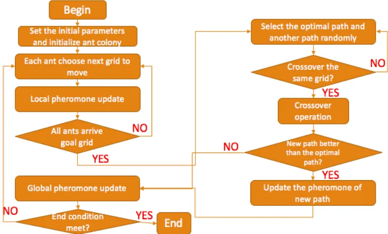
FIGURE 8: The flow chart of GA-ACA.

4.3 Robot path planning based on ACA-GA

4.3.1 Introduction of ACA-GA

The GA-ACA algorithm introduced in 4.2 apply GA and ACA in two stages

essen-tially, rather than an integration of these two algorithms in the true sense. In this

section, we will integrate into solution of ant colony optimization algorithm an idea

of crossover about genetic algorithm. The main framework of this algorithm is ACA,

but it integrates with GA during the intermediate solution process. To distinguish

this new algorithm with GA-ACA, we call it ACA-GA.

In short, ACA-GA selects two paths randomly after one iteration, and do the

crossover operation on two paths, and update pheromone of new path if it is better

than the optimal path in current iteration.

The crossover operation in the genetic algorithm is introduced into the ant colony

optimization algorithm, which can increase the diversity of the solution and speed up