ABSTRACT
XUE, XIANGZHONG. Electronic System Optimization Design via GP-Based Surrogate Modeling. (Under the direction of Dr. Paul D. Franzon.)
For an electronic system with a given circuit topology, the designer’s goal is usually to
automatically size the device and components to achieve globally optimal performance while
at the same satisfying the predefined specifications. This goal is motivated by a human desire
for optimality and perfection.
This research project improves upon current optimization strategies. Many types of
convex programs and convex fitting techniques are introduced and compared, and the
evolution of Geometric Program (GP)-based optimization approaches is investigated through
a literature review. By these means, it is shown that a monomial-based GP can achieve
optimal performance and accuracy only for long-channel devices, and that a piecewise linear
(PWL)-based GP works well only for short-channel, narrow devices without many data
fitted. Based on known GP optimizer and convex PWL fitting techniques, an innovative
surrogate modeling and optimization algorithm is proposed to further improve performance
accuracy iteratively for a wide transistor with a short channel. The new surrogate strategy,
which comprises a fine model and a coarse model, can automatically size the device to create
a reusable system model for designing electronic systems and noticeably improving
prediction accuracy, particularly when compared to the pure, GP-based optimization method.
To verify the effectiveness and viability of the proposed surrogate strategy, a widely used
optimal results of both coarse and fine models in the proposed surrogate strategy may
gradually converge to each other iteratively while achieving over 10% improvement in
performance accuracy compared to the previous, PWL-based GP algorithm. As a result, the
proposed surrogated modeling and optimization algorithm can serve as an efficient Computer
Aided Design (CAD) tool, with the capability of dramatically improving performance for
© Copyright 2012 by Xiangzhong Xue
Electronic System Optimization Design via GP-Based Surrogate Modeling
by
Xiangzhong Xue
A dissertation submitted to the Graduate Faculty of North Carolina State University
in partial fulfillment of the requirements for the degree of
Doctor of Philosophy
Electrical Engineering
Raleigh, North Carolina
2012
APPROVED BY:
_______________________________ ______________________________
Dr. Paul D. Franzon Dr. Michael B. Steer
Committee Chair
________________________________ ________________________________
DEDICATION
BIOGRAPHY
Xiangzhong Xue was born on July 17, 1976 in Chongqing, China. In 1997, he received a
Bachelor of Science degree from Chongqing University in China. He later moved to the
United States and studied at North Carolina Agricultural and Technical State University in
Greensboro, North Carolina, graduating with an Master of Science from the Department of
Electrical and Computer Engineering in August 2003. Continuing his doctoral work at North
Carolina State University in Raleigh, North Carolina, he graduated in May of 2012 with a
ACKNOWLEDGMENTS
This dissertation would not have been possible without the great help and encouragement
of my advisor, Dr. Paul D. Franzon, whom I most sincerely and deeply thank for all he has
done to help me in my studies and my life. I will always be grateful, too, for the guidance I
received from Dr. Michael B. Steer, Dr. Rhett Davis, and Dr. Harvey Charlton.
A special warm thanks to my wife, Xiuqiong Liu; my son, Ziang Xue; and all of my
friends for their continued support, care, and assistance.
An expression of sincere gratitude is extended to all my roommates, who have provided
me with generosity, help, and friendship through my time in Raleigh. I could not mark the
occasion without acknowledging them.
Finally, in appreciation for a lifetime of support and encouragement, I would like to thank
TABLE OF CONTENTS
List of Tables ... viii
List of Figures ... ix
Chapter 1 Introduction ... 1
1.1 Background and Motivation ... 1
1.2 Research Objectives ... 3
1.3 Research Contributions ... 3
1.4 Dissertation Organization ... 6
Chapter 2 Convex Program ... 8
2.1 Overview and Induction ... 8
2.2 General Mathematical Optimization Problem ... 9
2.3 Conic Programs ... 10
2.4 Convex Programs ... 11
2.4.1 Convex Set and Convex Function ... 13
2.4.2 Convexity Verification ... 14
2.4.3 Theoretical Properties ... 18
2.4.4 Numerical Solution Algorithms ... 20
2.4.5 Applications ... 20
Chapter 3 Geometric Program ... 22
3.1 Evolution of Geometric Programming ... 22
3.2 Standard Geometric Program ... 25
3.3 Relevant Terminology for the Geometric Program ... 26
3.3.1 Monomial Functions and Examples ... 26
3.3.2 Posynomial Functions and Examples ... 27
3.3.3 Inverse Posynomial Functions and Examples ... 28
3.3.4 Generalized Posynomial Functions and Examples ... 29
3.3.5 Signomial Functions and Examples ... 30
3.4 Transformation Methods for the Geometric Program ... 30
3.4.1 GP-compatible Algebraic Transformation ... 31
3.4.2 Fractional Powers of Posynomials ... 33
3.4.3 Maximum of Posynomials ... 35
3.4.4 Function Composition ... 36
3.4.5 Additive Log Terms ... 39
3.4.6 Generalized Posynomial Equality Constraints ... 40
3.4.7 Application Example: Geometric Program in Convex Form ... 44
3.5 Optimization Sensitivity Analysis ... 47
3.5.1 Tradeoff Analysis ... 47
3.6 Convex Approximation and Fitting ... 52
3.6.1 Convex Approximation and Fitting Theory ... 53
3.6.2 Monomial Fitting ... 57
3.6.3 Extended Monomial Fitting ... 59
3.6.4 Max-monomial Fitting ... 60
3.6.5 Posynomial Fitting ... 63
3.6.6 Convex Piecewise-Linear (PWL) Fitting ... 64
3.7 Methods for Solving Geometric Programs ... 66
3.8 Generalized GP and Relevant Solution Methods ... 69
3.9 Signomial Problem and Relevant Solution Methods ... 71
3.10 Summary ... 74
Chapter 4 Some Reviews of Analog Optimization Design ... 75
4.1 Introduction ... 75
4.2 GP-compatible Bias Description Techniques ... 75
4.2.1 Bias Condition Description with PF Equalities ... 76
4.2.2 Techniques for Converting PF Equality Constraints ... 78
4.3 Reviews of Two Analog Optimization Designs ... 80
4.3.1 Circuit Topology, Optimization Objective and Specifications ... 81
4.3.2 Hershenson's Work ... 82
4.3.3 Kim's Work ... 83
4.4 GP-compatible Device Model ... 86
Chapter 5 GP-Based Surrogate Modeling and Optimization Algorithm ... 90
5.1 Surrogate Theory ... 90
5.2 GP-based Surrogate Strategy ... 93
5.3 Design Case Study ... 95
5.3.1 Two-Stage Op-amp Design ... 96
5.3.2 LC-Tuned Oscillator Design ... 104
Chapter 6 Conclusion and Future Work ... 112
6.1 Conclusion ... 112
6.2 Future Work ... 117
References ... 119
Appendices ... 132
Appendix A Convexity of Point-wise Maximum of Convex Function ... 133
Appendix B Norm Approximation in Function Fitting ... 134
B.3 The Chebyshev orL Norm Approximation ... 136
B.4 The Hölder or LpNorm Approximation ... 136
B.5 Largest kterm Norm ... 140
Appendix C Optimization Objective and Specifications for Two-Stage Op-amp ... 141
Appendix D Preparation for LC-Tuned Oscillator Optimization Design ... 143
D.1 Analysis of Typical RLC Oscillator ... 143
D.2 LC-Tuned Oscillator Model ... 148
D.2.1 Transistor Model ... 149
D.2.2 Spiral Inductor and Varactor Model ... 150
D.2.3 LC-Tank Model ... 152
D.3 Design Specifications ... 156
D.3.1 Power Dissipation ... 156
D.3.2 LC-Tank Switching Voltage ... 156
D.3.3 Phase Noise ... 157
D.3.4 Resonant Frequency ... 160
D.3.5 Tuning Range ... 161
D.3.6 Inverses Loop Gain ... 162
D.3.7 Varactor Tuning Range ... 163
D.3.8 Bias Condition ... 163
LIST OF TABLES
Table 4.1 Comparison btw. two results from GP optimizer and 0.6µm SPICE tech ... 83
Table 4.2 Comparison btw. two results from GP optimizer and 0.18µm SPICE tech ... 83
Table 4.3 Max/Mean MF modeling error in GP model ... 84
Table 4.4 Discrepancy in specifications of two-stage op-amp design ... 84
Table 4.5 NMOS modeling error in TSMC 0.18um technique ... 84
Table 4.6 CPWL and MF-based optimization by GP & SPICE... 84
Table 4.7 Coefficients and exponents of Cgs of PMOS transistor with Vbs ... 87
Table 4.8 Mean modeling error of design parameters in TSMC 0.18µm technology ... 89
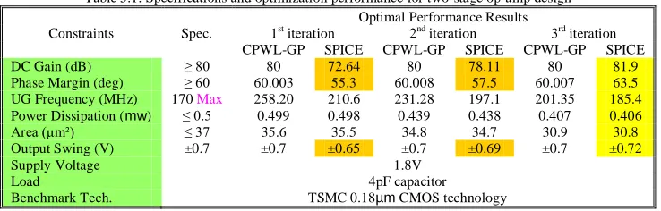
Table 5.1 Specifications & optimization performance for two-stage op-amp design ... 96
Table 5.2 Optimal performance for two-stage op-amp with different specifications ... 104
Table 5.3 Model expressions of optimization objective and specifications in LC-tuned oscillator ... 106
LIST OF FIGURES
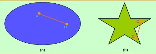
Figure 2.1 Examples of (a) convex set and (b) non-convex set ... 13
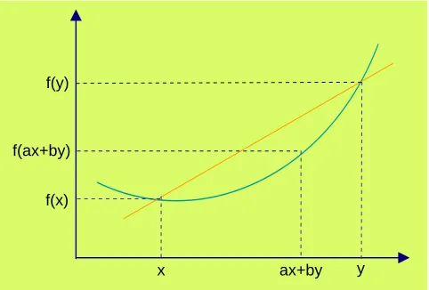
Figure 2.2 Convex function illustration ... 14
Figure 2.3 Three functions in (2.10) depicted on log-log scale ... 16
Figure 3.1 Function f(x)atan(x)and its least-square monomial fitting ... 59
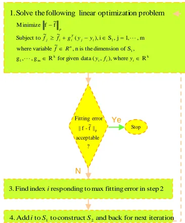
Figure 3.2 Procedures of convex PWL fitting algorithm ... 66
Figure 4.1 Common-source op-amps with PMOS active load ... 77
Figure 4.2 Two-stage op-amp optimization design ... 81
Figure 4.3 (a) NMOS transistor without Vbs (b) PMOS transistor without Vbs (c) PMOS transistor with Vbs operating in saturation region used for creating PWL and monomial device models ... 85
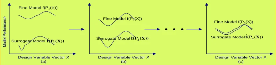
Figure 5.1 Evaluation of convergence of two model performance in surrogate strategy (a) initial design; (b) second design; (c) nth design ... 93
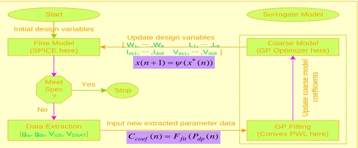
Figure 5.2 Surrogate modeling and optimization design flow ... 94
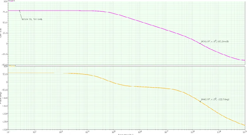
Figure 5.3 Optimal low frequency gain and phase margin at 1st iteration ... 97
Figure 5.4 Optimal low frequency gain and phase margin at 2nd iteration ... 99
Figure 5.5 Optimal low frequency gain and phase margin at 3rd iteration ... 100
Figure 5.6 Tradeoff curve of bandwidth vs. core area at 1st iteration ... 101
Figure 5.7 Tradeoff curve of bandwidth vs. core area at 2nd iteration ... 101
Figure 5.8 Tradeoff curve of bandwidth vs. core area at 3rd iteration ... 102
Figure 5.9 LC-tuned oscillator optimization design ... 105
Figure 5.10 Circuit-simulation-based phase noise of LC-tuned oscillator at 1st iteration ... 108
Figure 5.11 CPWL optimal phase noise of LC-tuned oscillator at 1st iteration ... 108
Figure 5.12 Circuit-simulation-based phase noise of LC-tuned oscillator at 2nd iteration .. 109
Figure 5.13 CPWL optimal phase noise of LC-tuned oscillator at 2nd iteration ... 110
Figure 5.14 Circuit-simulation-based phase noise of LC-tuned oscillator at 3rd iteration ... 110
Figure 5.15 CPWL optimal phase noise of LC-tuned oscillator at 3rd iteration ... 111
Figure D.1 Analysis of typical RLC oscillator (a) LC tank (b) Equivalent circuit of LC tank (c) LC tank with negative transconductance compensating the ohmic loss .. ... 143
Figure D.2 LC-tuned oscillator ... 148
Figure D.3 Small signal model of NMOS transistor ... 149
Figure D.4 Small signal analysis of cross NMOS couple ... 150
Figure D.5 Square spiral inductor used in LC-tuned oscillator ... 151
Figure D.6 Small signal of LC-tuned oscillator ... 152
Figure D.7 Reduced small signal of LC-tuned oscillator ... 153
Chapter 1
Introduction
1.1 Background and Motivation
Since the early 1960s, electronic Integrated Circuits (ICs) have become increasingly
complex. One particular trend is that the number of components in a single Integrated Circuit
(IC) doubles every 18 months, as predicted by Moore’s law [1]. Some current ICs, for
example, may contain devices that number in the hundreds of millions, with an equivalent
number of interconnected wires [2]; another trend is the rapidly increasing use of
mixed-signal ICs in fields such as telecommunications, computing, and automotive engineering [3].
Such an increase in design complexity, along with a growing demand for faster production
and greater cost effectiveness in a highly competitive market, strongly point to the need for
an innovative electronic design automation (EDA) and for new Computer Aided Design
(CAD)technologies for use in designing complex electronic systems.
Although the key component in EDA and CAD tools is the optimization engine, this
engine is often driven by outdated optimization algorithms. The optimizers used in SPICE,
for instance, are over 20 years old [4]. Thus, the focus of this work is to suggest a novel
approach to automatic optimization techniques. The optimizers within the proposed
optimization engine are expected to be capable of effectively handling large numbers of
design variables and constraints, as well as wide stochastic uncertainty and variation,
The literature on the subject of CAD technologies for ICs is extensive. A good survey of
early research can be found in [2].More recent papers include [3], [5], and [6]. Among
existing techniques, the geometric program (GP)-based method has recently received close
attention. Much work has been done, for example, on optimizing switched-capacitor filters
[7], pipelined Analog-to-Digital Converter (ADC) design [8], Phase Lock Loop (PLL) design
[9], and Direct Current to Direct Current (DC-DC) buck converter design [10]. Significantly,
researchers have found that the GP-based method has overwhelming advantages in that it
always automatically finds the globally optimal solution (if it exists), is extremely fast, and is
independent of the initial point.
However, the geometric program approach still has several drawbacks, in that it requires
a posynomial function (PF) type of objective and inequality and has monomial function (MF)
equality constraints. Still, transistor characteristics in models such as BSIM3v3 are usually
highly non-convex, so convex fitting techniques such as monomial fitting and convex
piecewise linear (PWL) fitting are needed to formulate a GP-compatible model. The
approximation inevitably leads to some level of error. Work [11] shows that a monomial
fitting is suitable only for long-channel transistors, but not accurate enough for short-channel
devices. Work [12] uses a convex PWL fitting for short-channel but narrow transistors with a
small number of design parameter data fitted, and as a result higher fitting accuracy is
achieved. However, our work shows that such an approach no longer works effectively for
wide transistors when fitting a large amount of parameter data, and thus a way must be found
1.2 Research Objectives
To handle the rapid increase in design complexity, the greater demand for design-to-market
time reduction, and the need for greater cost effectiveness in a highly competitive market,
innovative EDA and CAD technologies are highly encouraged [3]. Also, for an electronic
system with a given circuit topology, the designer’s typical goal is to automatically size the
devices and components to achieve globally optimal performance while at the same time
satisfying the predefined specifications. This goal is motivated by an inherent human desire
for optimality and perfection. Consequently, this work will concentrate on proposing novel
EDA and CADtools. The resulting innovation should have the following noticeable features.
It can completely and automatically size the devices and components in the designing
electronic system to save the designer from the tedious and time-consuming work of
device-size tuning, enabling the designer to focus on more important design tasks
such as analyzing the trade-off between the competing objectives and constraints.
The proposed CAD tool should be embedded with an powerful optimizer, which will
find the existing globally optimal design automatically and extremely fast, directly
from the given specifications and independent of the initial design point.
The achieved final design should have high performance and accuracy compared with
current EDA and CAD tools.
1.3
Research Contributions
As stated earlier, among those existing EDA and CAD techniques for IC design, the
unmatched advantages: always finds the existing globally optimal solution automatically and
efficiently regardless of the initial point [7, 8, 9, and 10]. This meets the first two desired
features of an IC design CAD tool. Consequently, such an automatic and efficient optimizer
is embedded in our proposed CAD tool.
The GP approach requires a special format: posynomial objective, posynomial inequality
constraints, and monomial equality constraints [13]. However, today’s transistor
characteristics are highly non-convex, so convex fitting techniques are needed to formulate a
GP-compatible device model. Here, a convex PWL (CPWL) fitting technique is selected in
our proposed CAD tool to derive a GP-compatible device model because it can achieve quite
high fitting accuracy compared with many convex fitting techniques such as monomial fitting.
But our work shows that convex PWL fitting is not accurate enough for an electronic system
involved with wide transistors when fitting a large amount of parameter data. In this work,
we adopt the strategy of surrogate modeling to further enhance the performance accuracy
iteratively. Then our proposed CAD tool can achieve high performance and accuracy, the
third desired feature of an IC design CAD tool.
In summary, the contribution that our work makes in this field is that, based on GP
optimizer and CPWL fitting technology, we propose an innovative Surrogate Modeling and
Optimization algorithm (SMOA) to further enhance the performance and accuracy of the
electronic system optimal design iteratively and automatically. This proposed surrogate
strategy can serve as an efficient EDA and CAD tool with dramatic performance
improvement for electronic system optimal design compared with existing similar tools. As
For the first time, the surrogate models are created with a convex piecewise linear
(CPWL)-based GP. This proposed modeling and optimization tool inherits from GP
its high efficiency and the ability to find the globally optimal design. It also benefits
from the CPWL fitting technique to achieve high fitting precision. This better initial
surrogate model established with such high-fidelity fitting techniques will be very
helpful in reducing the number of total used iterations.
In the modeling methods current today, the system models are created relying on the
design parameter information of a single device model (for example, [11] and [12]).
The problem with this method is that such design parameter information is isolated
from the actual designing electronic system. In contrast, except for the first iteration,
we extract the needed design parameters directly from fine model of the designing
electronic system. These extracted parameter data are directly related to the designing
electronic circuit system, and they have much more relevant physical and electrical
information about the designing circuit system. Establishing a more accurate
surrogate model would thus be highly beneficial. In addition, it reduces the
discrepancy between the surrogate model and the fine model. Furthermore, the
number of iterations is reduced, and the design time is cut accordingly.
To ensure the convergence between both the fine model and the surrogate model, and
to increase the convergence speed, some matching constraints and Jacobean
conditions, denoted by a reflection functions , can be imposed between the optimal
optimization design variables of the fine model from the optimal value of the
optimization design variables in the surrogate model through the relationship
) x ( 1)
x(n
This will guarantee that we will achieve the optimization design of the designing
electronic system while meeting all the required specifications.
To get a sequence of optimization design variable points, we choose to sweep one or
more design variables. The sweep is very flexible. For convenience, only one design
variable (bias current) is swept in both design study cases.
1.4 Dissertation Organization
This work has six chapters. The introduction begins with a background overview and a
description of our research motivation for improving design automation and CAD tools for
IC optimization design. Next, the objectives of this work are stated, along with the original
contributions it will make in the field. Chapter 2 introduces the convex program (CP) and
some of its variations, some involved transformations, and fitting technologies. Chapter 3
introduces geometric programming (GP), a special optimization method playing an important
role in two previous research works [11 and 12]. It also describes two involved convex fitting
techniques: the monomial fitting and convex piecewise linear (PWL) fitting technologies
used in [11] and [12]. The GP optimizer and the convex PWL are also one basis of this work.
Chapter 4 reviews two previous works [11 and 12] and analyzes the optimization algorithms
and fitting technologies used in them; the modeling accuracy achieved by monomial fitting
major prediction error sources are also analyzed. Chapter 5 proposes a surrogate modeling
and optimization strategy based on the GP optimizer and convex PWL fitting technique to
further improve the performance accuracy. Its key idea and procedures are described in
detail. Two design examples are also carried out to verify the effectiveness and viability of
the proposed surrogate modeling and optimization algorithm. Chapter 6 states our
Chapter 2
Convex Programs
2.1
Overview and Introduction
Human beings have an inherent desire for their tools and technologies to perform with
optimal efficiency and perfection. The search for extremes has inspired mountaineers,
scientists, mathematicians, and the rest of humanity since the beginning of history [14].
Optimization techniques can help humans and machines make decisions as they approach
goals that have been set in response to a given problem [15]. As a result, various design
solutions can be realized: designs for minimal operating cost, maximum profit, minimum
loss, minimum consuming fuel, optimal product quality, smallest device size, optimal
strategy, optimal path, optimal trajectory, optimal orbit, aerospace trajectory optimization,
optimal surface, optimal overall performance, and other goals.
The rapid development of optimization techniques began during World War II when such
techniques were needed to optimize the trajectories of missiles [16]. Subsequently,
mathematical programming has been developed to realize optimization through the
application of mathematical techniques. A beautiful and practical mathematical theory of
optimization (i.e. search-for-optimum strategies) emerged rapidly in the 1960s, when
computers became widely available. For example, the optimization of meta-heuristics, which
imitates physical phenomena and the evolution of living organisms, has been in development
problems and call for new methods. The goal of the optimization theories is the creation of
reliable methods to catch the extremum of a function by an intelligent arrangement of its
evaluations (measurements). In the past, new optimization techniques had been developed in
each era in order to realize customer solutions. Now, however, those optimizations have
become dated, and new solutions must be realized. For example, the system optimization
engine in SPICE, an important popular circuit Computer Design Automation (CAD) tool, is
still driven by an optimization algorithm that is over 20 years old [5].
Up-to-date optimization theories are vitally important for modern engineering and
planning that incorporate optimization at every step of the complicated decision making
process [14]. Hence, this chapter introduces some recent optimization techniques and their
practical applications, but without emphasizing the theoretical optimization knowledge or
reviewing classical optimum methods, such asConjugate Gradients, the Newton Method, and
methods for constrained and unconstrained optimization including Linear and Quadratic
Programming. Specifically, several types of optimization programs are introduced for the
purpose of comparison, with a focus on the most widely used one, the convex program. This
program has recently been used in a variety of fields—for example, control engineering,
signal processing, circuit design, economics, finance, and communication and information
theory.
2.2
General Mathematical Optimization Problem
First we will introduce the general optimization problem. A general optimization problem
x nh
m x
g x f
j i
, , 1 j 1
, , 1 i 1
subject to
minimize 0
(2.1)
The vector xRnis the optimization variables; the function f0:xRis the objective
function which will be designed or realized; the functions gi(x)1 and hj(x)1are the
involved inequality and equality constraints, respectively.
Specifically, for an optimization problem the objective is to find such an optimal solution
*
x that f0(x*)is the minimum (the maximum is also possible in some cases) satisfying the set of constraints gi(x)1 and hj(x)1, which reflect the requirements on the expected
products and/or the limited situations and technologies that are currently available. Since the
exact optimal solution cannot always be found for a real time optimization problem, we often
try to achieve a practical near-optimal solution xˆ within a predefined error tolerance such that f0(xˆ) f0(x*) .
2.3
Conic Programs
One family of optimization problems that has become quite common is the primal and its
corresponding dual conic programs [13]:
x
m b
Ax x c
, , 1 i ,
subject to
minimize T
(2.2)
} n , , 1 , 0 | {
Rn x Rn xj j (2.3)
Two conic forms dominate recent study and implementation. One is the semi-definite
program (SDP), for which is an isomorphism of the cone of positive semi-definite matrices: } 0 ) ( |
{ min
X X R X
Sn T n n (2.4)
The second is the second-order cone program (SOCP), for which is the Cartesian product of one or more second-order or Lorentz cones:
} | ) , {(
, n 2
nk
1 x y Rn R x y
n
(2.5)
SDP and SOCP receive this focused attention because many applications have been
discovered for them, and because their geometry admits certain useful algorithmic
optimizations [19, 20, and 21]. Publicly available solvers for SDP and SOCP include [22, 23,
and 24]. These solvers are generally quite efficient and reliable, and they require no external
code to perform function calculations.
2.4
Convex Program
Another very important mathematical optimization problem is called convex program, which
has the following form [17]:
p x g m x f x f j i , , 1 j , 1 ) ( , , 1 i , 1 ) ( subject to ) ( minimize 0
(2.6)
Compared with general optimization problems, the convex problem has the following
The objective function must be convex.
The inequality constraint functions must be convex.
The equality constraint must be affine.
A convex program (CP) is special case of (2.1): the objective function and inequality
constraint functions fi(x) are convex, and the equality constraint functions gj(x) are monomial.
It is necessary to know that when the convex program is used to design an electronic
system in practice, the design variablexshould satisfy the constraints ofx0because it usually represents the device size and component value of the designing electronic system.
One important property of the convex program is that the feasible set of a convex
optimization problem is convex because it is the intersection of the domain of the problem.
mi
i
domf D
0
(i0,,m)
Therefore, a convex optimization problem turns out to minimize the convex objective
function over a convex set, and thus any local optimal point is definitely globally optimal,
which is an overwhelming advantage over general nonconvex optimization problems.
Another fact, which is worth knowing, is that although it is not obvious, a convex
program can be reformulated as a conic program by selecting appropriatein (2.2) [13]. Certain special cases of (2.6) receive considerable attention. By far the most common is
the linear program, for which the functions fi, gjare all affine; e.g.,
m b
Ax x c
, , 1 i
subject to
minimize T
Similarly, when an LP is used to design a practical electronic system, there should be an
extra constraint on the design variables: that is,x0because it is the device size and the component value of the designing electronic system.
Quadratic programs (QPs) and least-squares problems can be expressed in this form as
well. The class of nonlinear programs (NLPs) includes nearly all problems that can be
expressed in the form (2.1) withxRn, although generally there are assumptions made about
the continuity and/or differentiability of the objective and constraint functions. The set of
CPs is a strict subset of the set of NLPs, and includes all LPs, convex QPs (i.e., whose
Hessian 2f is positive semi-definite), and least-squares problems. Several other classes of
CPs have been identified recently as standard forms. These include second-order cone
programs [26], and geometric programs [27, 28, and 29].
2.4.1 Convex Set and Convex Function
A setCRnis convex [18] if the line segment between any two points inCstill lies inC, i.e., C
θ)x (1 θx 1 θ 0 C, x ,
x1 2 1 2 (2.8)
For example, the set (a) in Figure 2.1 (below) is convex set but the set (b) is nonconvex
because the line segment lies outside of the set.
A
B
C D
(a) (b)
Accordingly, a function f :Rn Ris convex if its domain is a convex set and this function satisfies the inequality condition (2.9),
) ( ) ( )
(ax by af x bf y
f (2.9)
for all x,yRn and all a,bRwithab1, a0, b0. Geometrically, inequality (2.9)
means that the line segment between(x,f(x))and(y,f(y)) lies above the graph of f as
shown in Figure 2.2.
x y
f(ax+by)
ax+by f(y)
f(x)
Figure 2.2: Convex function illustration
2.4.2 Convexity Verification
Apparently, the convexity verification of the objective function and the constraint functions
is important for testing a convex program optimization problem. Unfortunately, it can be
difficult to determine whether a function with many variables is convex (or nearly convex).
In general, this task is at least as difficult as solving nonconvex problems: that is, it is
In this section, we introduce some techniques that can be used to prove or disprove
convexity of a general functionF(y)log( f(x)), whereylogx is a n-dimensional variable
vector [30].
Method 1: Check the curvature of the testing function
For the special casen1, the convexity of a function F(y)is readily determined by simply plotting this function and checking whether it has positive (upward) curvature. This is
the same as plotting f(x)on a log-log plot, and checking whether the resulting graph has
positive curvature. If the curvature of the function is curved, then it is convex; if this curve is
straight, then it is affine, and also convex; otherwise, it is not convex.
For high-dimension functions, a function is convex only if it is convex when restricted to
any straight line. In other words, one can plot F(y0tv)versust, for various values of
0
y andv. If any of these plots exhibits negative (i.e., downward) curvature, thenF is not convex. In this way, it is not easy to directly prove that a high-dimension function is a
convex function.
The following three functions of one variable in (2.10) are demonstrated here as an
example of verifying the convexity of a function,
1
4
x ,atan(x) andx31 (2.10)
These functions are plotted over the range 0.1x1on a log-log scale in Figure 2.3. From the figure one may see that the first function is convex since its graph is an upward
curve on this log-log plot; the second is also convex because its graph is relatively straight.
10-1 100 -4
-3.5 -3 -2.5 -2 -1.5 -1 -0.5 0 0.5 1
f1(x) = x4+1 f2(x) = atan(x)
f3(x) = -x3+1
Figure 2.3: Three functions in (2.10) depicted on log-log scale
Method 2: by verifying the inequality condition (2.9)
A function f :Rn Ris convex if domain of f ,dom , is a convex set andf f satisfies )
( ) ( )
(ax by af x bf y
f
for all x,yRn and all a,bR with ab1, a0 , b0. Similarly, the convexity ofFcan be stated in terms of the original function f . This means that f must satisfy the inequality (2.11),
1
1 1
1 1
1
1 )
~ , ... , ~ ( ) , ... , ( ) ~ , ... , ~
(x x xnxn f x xn f x xn
f (2.11)
for anysatisfying0 1. In other words, when f is evaluated at a weighted geometric mean of two points, it cannot be more than the weighted geometric mean of the function
f evaluated at the two points.
Method 3: by checking the first or second-order conditions (i.e., gradient functionf and
Hessian function ∆2f) of the testing function, i.e., ) ( ) ( ) ( )
(y f x f x y x
or
2f(x)0xdomf (2.13)
This test method can be stated as the following results:
If all Hessians of function f are positive semi-definite over the feasible region, the
problem is convex.
If any Hessian of function f is negative definite over the feasible region, the problem
is nonconvex.
Otherwise (i.e., any Hessian of function f is semi-negative definite), no conclusion
can be made.
Note that the third case does not mean that the problem is convex or non-convex, only that
the system was unable to reach a conclusion.
For example, linear functions are convex because their second derivative is zero,
therefore satisfying (2.13).
Another example is to prove the convexity of the logarithmic function of a PF with
Method 3.
If posynomial function f is expressed in the form of
m
i
n i
ni i ix x x
c x
f
1
2
1 ...
2
1
After introducing the logarithmic transformyi logxi, (that is yi
i e
m i b y a m i y y y i m i n i i i n i i i n i i i e e e e c x x x c x f 1 1 1 2 1 ) ...( ) ( ) ( ... 1 2 1 1 1 2 1 whereai (1i,2i,,ni), bi logci andy(y1,y2,,yn)T. This is a so-called sum-exp function f(x)e1 en, here
i i
i ayb
. Then its logarithmic function F(x) is a
so-called log-sum-exp functionF(x)log(e1 en). Now we can verify the convexity of the log-sum-exp function with Method 3, first by computing its Hessian as
) ) ( ) 1 (( ) 1 ( 1 ) ( 2
2 T T
T z diag z zz
z x
f
wherez(e1,,en), then by proving2f(x)0which is to check that vT2f(x)v0for allv, i.e.,
0 ) 1 ( 1 ) ( 2 1 1 1 2 2 2
n i i i n i i n i i i T T z v z z v z v x f vThis result can be guaranteed by the Cauchy-Schwarz inequality 2
) ( ) )(
(aTa bTb aTb with
valueai vi i , andbi i .
2.4.3 Theoretical Properties
Here we survey and introduce some theoretical properties of convex programs. By the 1970s,
a comprehensive theory of convex analysis had appeared [31, 32], and advances continue
First of all, the local optima of a convex program are also definitely global optima
because, as stated previously, the domain of any convex program is the intersection of the
domain of some convex inequality constraints and affine equality constraints. However, this
is not the case for general nonconvex NLPs. A general nonconvex NLP may have multiple
local optima, so it usually needs exhaustive computation to verify whether each local optima
is global. Convex programming also has a rich duality theory. The dual of a CP is itself a CP,
and its solution often provides interesting and useful information about the original, or
primal, problem. For example, if the dual problem is unbounded, then the primal must be
infeasible. Under certain conditions, the reverse implication is also true: If the primal is
infeasible, then its dual must be unbounded. These and other consequences of duality
facilitate the construction of numerical algorithms with definitive stopping criteria for
detecting infeasibility, unboundedness, and near-optimality. In addition, the dual problem
provides valuable information about the sensitivity of the primal problem to perturbations in
its constraints. A more complete development of convex duality can be referred to [31, 21].
Another important property of CPs is the provable existence of efficient algorithms for
solving them. Nesterov and Nemirovsky proved that a polynomial-time barrier method can
be constructed for any CP that meets certain technical conditions [35]. Other authors have
shown that the problems that do not meet those conditions can be embedded into larger
problems that do, effectively making barrier methods universal [21, 36].
Note that the theoretical properties discussed here, including the existence of efficient
solution methods, hold even if a CP is non-differentiable: that is, if one or more of the
2.4.4 Numerical Solution Algorithms
Some efficient algorithms for solving CPs have been known since the 1970s, but only in the
last two decades have some practical advances been made. Among those algorithms, interior
point methods [37, 38] have attracted the attentions of many researchers because these can
always, and very efficiently, find the existing globally optimal solution. At the first stage, this
method was limited to LPs [39, 40, 41], but soon it extended to other CPs [42, 43, 44, and
45], especially by Dr. Stephen P. Boyd and his research team. Now a number of excellent
solvers are readily available in two classes: those relying on standard forms and those based
oncustom code.
2.4.5 Applications
Many practical applications for convex programming have already been discovered, and the
list is steadily growing. Perhaps the most mature and pervasive field of the application for
convex programming is control theory [46, 47, and 48]. Other fields where applications of
convex optimization have been developed include robotics [49, 50], combinatorial
optimization and graph theory [51, 52, 53, 54], structural optimization [55, 56, 57, 58],
algebraic geometry [59, 60], signal processing [61, 62, 63, 64, 65, 66, 67], communications
and information theory [68, 69, 70], networking [71, 72], circuit design [73, 74, 11, 75],
neural networks [76], and economics and finance [77, 78].
This list is certainly incomplete, and it excludes applications where only LP or QP is
employed. A list including LP and QP would be significantly larger, and yet convex
A promising source of new applications for convex programming is the extension and
enhancement of existing applications for linear programming. An example of this is robust
linear programming, which allows uncertainties in the coefficients of an LP model to be
accounted for in the solution of the problem, by transforming it into a nonlinear CP [25]. This
approach produces robust solutions more quickly and reliably than the Monte Carlo methods.
Some may argue that our prognosis for the usefulness of convex programming is
optimistic, but there is good reason to believe that the number of applications is in fact being
underestimated. We can appeal to the history of linear programming as precedent. George
Dantzig first published his invention of the simplex method for linear programming in 1947;
and while a number of military applications were soon found, it was not until 1955-1960 that
the field enjoyed robust growth [79]. This delay was in large part due to a dearth of adequate
computational resources, but that is precisely the point: The discovery of new applications
accelerated only after hardware and software advances made it truly practical to solve LPs.
Thus, for applications relating to one special convex program—the geometric program—
one can see the importance of the two optimization designs addressed in this work, the
Chapter 3
Geometric Programming
There is another special standard form of optimization problem (2.1): the geometric program
(GP). Although a geometric program can be converted to a convex program after logarithmic
transformation, its discussion merits a whole chapter because of its rapidly increasing use in
a wide variety of fields and the renewed interest it has generated recently. Moreover, it is
used as one basis of the proposed modeling and optimization strategy in this work. This
optimization program is thus discussed in detail here.
The specialty of GP is that its objective and constraint functions are posynomial and
monominal functions of the design variables [17]. Once again, GP does not directly fall into
the category of convex programs, but a simple logarithmic transformation produces an
equivalent convex problem, which can then be solved with the efficient mature solvers
developed for convex optimization problems. The convertibility to a convex program has
profound advantages: It is highly efficient, and the global solution is always found regardless
of the initial point if the problem is feasible. The latter is, perhaps, an even greater advantage
than the high efficiency.
3.1
Evolution of Geometric Programming
Let us first give a brief introduction to the evolution of geometric programming. One pioneer
minimization problems in engineering can be stated in a special form and solved very easily
[80]. Almost at the same time, Richard Duffin, a Mathematics professor at Carnegie Mellon
University, was developing a duality theory for nonlinear programming problems. Duffin
learned of Zener’s work and started to construct a mathematical framework for geometric
programming based on his work on duality theory [81, 82]. A few years later, the two
pioneers published the book Geometric Programming, in 1967 [83]. This book set the
necessary groundwork for geometric programming. It includes the basic theory and some
electrical engineering applications (e.g., optimal transformer design), but not much on
numerical solution methods. The name ―geometric programming‖ was given by Duffin,
Peterson, and Zener in 1967 [83]. One might think that the name derives from the many
geometric problems that can be formulated as a geometric program; however, the name
comes from the extensively used geometric-arithmetic mean inequality, which played a
central role in the early analysis of the geometric program.
Since the late 1960s there has been extensive work done in both the theoretical and
practical aspects of geometric programming. Another two books appeared in the 1970s:
Engineering Design by Geometric Programming, by Zener [84] and Applied Geometric
Programming, by Beightler and Phillips [85]. In 1978 two issues of the Journal of
Optimization Theory and Applications were entirely devoted to geometric programming.
Additionally, there are several papers on methods for solving geometric programs. The 1980
survey paper by Ecker [86] has many references on applications and methods, including
numerical solution methods used at that time. Geometric programming is also briefly
Unfortunately geometric programming has been kind of an outcast in the optimization
community [89]. For years, the mathematical programming community has regarded
geometric programming as a mere curiosity. However, it has been enthusiastically embraced
by the engineering community. This great change took place in the 1990’s, led by Stephen
Boyd and his research team at Stanford University. They developed an efficient and mature
numerical solver for convex programs and geometric programs, and produced many works
on engineering applications, especially electronic system design [11, 67, 73, 74, and 75].
There are various applications of the GP. The following selected list shows some of the
range of applications. In Chemical Engineering: general problems [90], Williams Otto
process optimization [91], and condenser design [92]. In Civil Engineering: cofferdam design
optimization [93], structural design [94, 95], steel plate girders [96], and structural design of
aircraft wings [97]. In Economics: marketing-mix problem [98], inventory optimization [99,
100, 101], and maximization of profit rate [102]. In Electrical Engineering: transformer
design [93], digital circuit transistor sizing [11, 67, 73, 74, 75], and optimal floorplanning for
layout [103, 104]. In Environmental Engineering: wastewater treatment plants [105, 106],
and water treatment [107]. In Mechanical Engineering: optimal design of journal bearing
[108], space trusses [109], and helical spring [110]. In Nuclear Engineering: cooling-tower
system optimization [111]. In Communication Engineering: communication systems [18].
Obviously, geometric programming has had tremendous impact in various areas. It is
surprising and interesting that although geometric programming looks like a restrictive type
of optimization problem, it has been used to solve an extremely wide variety of practical
3.2
Standard Geometric Program
In this section, a powerful optimization method, called Geometric Programming, is
introduced for determining the component values and transistor dimensions in electronic
circuit system optimization design. This method can handle a very wide variety of
specifications and constraints extremely fast, and results in globally optimal designs [11, 67,
73, 74, 75, and 112].
A standard geometric program (GP) is an optimization problem of the form
n , , 1 , 0
p , , 1 , 1 ) (
m , , 1 , 1 ) ( Subject to
) (
M inimize 0
k x
j x g
i x f
x f
k j i
(3.1)
where x(x1,, xn) are the optimization design variables, the inequality constraint
functions fi , i0,,m , are posynomial, the equality constraints gj , j1,,p are
monomial functions, and all the optimization variablesxk, k 1,,nshould be positive. A geometric program can be reformulated as a convex optimization problem by taking the
logarithmic transformation of design variables. More details can be found in Section 3.4.8
later.
If the functions fi,i0,,m are generalized posynomials, problem (3.1) is called a
generalized geometric program (GGP). If any functiongjis signomial function, then problem (3.1) is called a signomial program. A geometric program is also a GGP because a
posynomial function is a special case of GGP, and a generalized geometric program can be
The GP has some unmatched advantages over many current IC optimization
technologies. First, it can handle large numbers of design variables and constraints, and it can
be reformatted as a convex optimization problem, then solved extremely fast by the
developed interior point methods [28, 113, and 114]. For example, systems involving tens of variables and hundreds of constraints can be solved in less than one second [114, 17]; and those with thousands of variables and tens of thousands of constraints are readily solved on a
small workstation in minutes [115].Perhaps more important than the great efficiency is that GP always obtains the globally—not locally—optimal solution (if it exists) no matter what
the initial point is. GP has naturally gained popularity in IC optimization design [11, 12].
However, this approach still has several limits. It does not provide much insight into the
failure of some specifications, nor does it suggest to the designer how to change the circuit
topology for better results. It also requires a special format and function: PF objective, PF
inequality, and MF equality. Exactly for this reason, some convex fitting techniques, such as
monomial fitting and convex PWL fitting, are often needed to derive GP-compatible device
models.
3.3
Relevant Terminology for the Geometric Program
In the following section, all of the terminology relevant to the geometric program will be
introduced to facilitate understanding.
3.3.1 Monomial Functions and Examples
n
n
x x cx x
f 1 2
2 1
)
( (3.2)
where the coefficientc0and the exponentsai R, is called a monomial function (MF) [17]. One should note the distinction between the MF defined here and the common algebra
definition: The former can be any real value, including negative and fractional, but the latter
should be a nonnegative integer. For example, 10.7x15.4x23.67x103 is a MF of the variables x1, x2 and x3 , with a coefficient of10.7 ; likewise, 5.1x3 xy/z is also a MF;
but1.8x13x72.4x32x144 is not, since its coefficient1.8is negative. One special case is that a positive constant such as 67.9 can be also considered an MF. Some properties of PF can be
stated as follows:
A positive constant is also a monomial.
MF is closed under multiplication and division: If two functions f1and f2are MFs,
their product f1 f2and quotient f1 f2are also MFs. Two special cases are that an
MF scaling by any positive constant is still MF and an MF raised to any power is also
an MF—that is, if function n
n
x x cx x
f( ) 1 2...
2 1
is an MF, then the scaled MF
n
n
x x bcx x f
b ( ) 1 2...
2 1
and raised power function m n
n m m m m
x x x c x
f( )] ...
[ 1 2
2 1
,where
0
b andmR, are still MFs.
3.3.2 Posynomial Functions and Examples
A sum of two or more monomial functions in the form of
m
i
n i
ni i ix x x
c x
f
1
2
1 ...
2
1
whereci 0, is called a posynomial function (PF) [116]. Some examples of PF are given here as 100.7, 1.8x13x27.4x32x144 and 14 3
4 2 3 4 . 7 2 3
1 5.1 /
8 . 1 92 .
4 x x x x x xy z , but the two functions
x xyz sec 53
.
4 and(xyz)52.56 are not PF. Some properties of PF can be listed as follows:
Any MF is also a special PF; PF is closed under addition, multiplication, and
nonnegative scaling.
If function f is a PF andmis a nonnegative integer, then fmis a PF because it is the multiplication of mPFs.
If function f1is posynomial and function f2is a monomial, then f1/ f2is a posynomial.
If function f is a PF, then its logarithmic transformation functionlog f is also PF.
3.3.3 Inverse Posynomial Functions and Examples
The reciprocal of a posynomial function with the format of
m
i
n i
n i i ix x x
c x
f
1
2
1 ...
1
2
1
(3.4)
is called an inverse posynomial function (IPF) [17]. For example, the
functions2/xand1/(2xy)are both IPFs.
An inverse posynomial function has following properties:
A monomial is also an inverse posynomial function.
Inverse posynomials are closed only under multiplication and nonnegative scaling.
3.3.4 Generalized Posynomial Functions and Examples
A generalized posynomial function (GPF) [116] is a function constructed from posynomial
functions using addition, multiplication, pointwise maximum, and raising to constant positive
power. From this definition, one can see that a PF is also a special GPF.
For example, the functions100.27x17.9x23.2 ,8.2(x1x12.37.4x12x24.17x33.910.605)4.511.8 and max{0.2x1x26.21,3.6x13.4x20.7,6.1x52.14x33/8x12x24.17x33.91}are all GPF. Some properties of PF can be stated as follows:
A MF is also a GPF; a PF is also a GPF.
GPF holds its closure under addition, multiplication, nonnegative scaling, positive
power and component maximum, as well as other operations that can be derived from
these, such as division by monomials. They are also closed under composition in the
following sense. If is a generalized function of kvariables, for which no variable occurs with a negative exponent, andh1(x),,hk(x)are GPF, then the composition function f(x)(h1(x),,hk(x))is a GPF.
If function f is a GPF andmis a nonnegative integer, then fmis a GPF.
If function f1is a GPF and function f2is a MF, then f1/ f2is a GPF.
If function f is a GPF of m variables with nonnegative exponent, and functions
i
g (i1,,m) are all GPF, then the composition function f(g1,,gm)is a GPF.
If function f(x) is a GPF, then the logarithmic transformation
3.3.5 Signomial Functions and Examples
In some cases, just as in an algebraic MF or PF, the coefficients are perhaps negative. In such
a case, we call a function in the form of
m
i
n i
ni i ix x x
c x
f
1
2
1 ...
2
1
(3.5)
whereciR, a signomial function (SF) [30]. An SF has the same format as a PF; however,
the coefficients in the former can be both positive and negative, whereas the coefficients in
the latter can be only positive. So a PF is also an SF. For example,
21 . 9
and(x1x22x3)38.25are both SFs. An SF has several properties:
A constant number is SF; an MF is also an SF; a PF is also an SF.
Any SF is the difference of two PFs by collecting together the terms with positive
coefficients and also the terms with negative coefficients.
SF is closed under addition, subtraction, and multiplication.
An SF divided by an MF or the negative of MF is still an SF.
A SF raised to a nonnegative integer power is also a SF.
3.4
Transformation Methods for the Geometric Program
Simple tricks and transformations allow one to handle a wider variety of optimization
problems by converting to a standard GP. In this section, some such transformations are
3.4.1 GP-compatible Algebraic Transformations
Scale transformation If function f(x) is a PF and kis a positive value, then the inequality constraint f(x)kcan be changed to the standard posynomial inequality constraint as
1 / ) (x k f
which is compatible with the standard geometric program. Similarly, if another
function g(x)is a monomial function, then the inequality constraint f(x)g(x)can be
converted to the equivalent standard posynomial inequality constraint
1 ) ( )
(x g x
f
which is also a posynomial constraint compatible in the standard geometric program [13].
Inverse transformation If function f(x)is an IPF and g(x)is posynomial, the inequality constraint f(x)g(x)can be transformed as a standard posynomial inequality constraint
1 ) ( 1 )
(
x f x
g .
through dividing by f(x)on both sides.
If function f(x) is an IPF and function g(x) is an MF or IPF, the inequality
constraint f(x)g(x)1can be converted as
1 ) ( 1 ) (
1
x g x
f
through dividing by f(x)g(x)on both sides. This resultant inequality is compatible with
If the objective function f0(x) is an IPF or MF, then one can maximize such an objective function by minimizing its inverse, which is a PF or MF, separately.
Monomial division transformation If function f(x)andg(x)are both MFs, then the equality constraint f(x)g(x)can be replaced by the equivalent standard equality constraint
1 ) ( )
(x g x
f org(x) f(x)1 [17].
An example is given here to demonstrate the basic GP model formulation and the
application of simple transformation methods. Suppose that we have a piece of rectangular
aluminum material, with sides wand l. The material is used to make a cylindrical container with as much volume as possible, denoted byV . The following requirements are delimited by the available budget: The material’s dimensions must be wmin wwmaxandlmin llmax, the material’s area should be no more thanSmax, the area of the cover should be no more
thanSmax1, and the side area of cylinder should be no more thanSmax2. What, then, are the available maximum volume and its equivalent dimensions? This is a simple optimization
problem, which can be extracted and expressed as follows: