Recent Advances in the Measurement of Rare-Earth Metal Transition Probabilities Using Laser-Induced Plasmas

(1)

University of Windsor University of Windsor

Scholarship at UWindsor

Electronic Theses and Dissertations Theses, Dissertations, and Major Papers

2014

Recent Advances in the Measurement of Rare-Earth Metal

Transition Probabilities Using Laser-Induced Plasmas

Russell Putnam

University of Windsor

Follow this and additional works at: https://scholar.uwindsor.ca/etd

Recommended Citation Recommended Citation

Putnam, Russell, "Recent Advances in the Measurement of Rare-Earth Metal Transition Probabilities Using Laser-Induced Plasmas" (2014). Electronic Theses and Dissertations. 5275.

https://scholar.uwindsor.ca/etd/5275

This online database contains the full-text of PhD dissertations and Masters’ theses of University of Windsor students from 1954 forward. These documents are made available for personal study and research purposes only, in accordance with the Canadian Copyright Act and the Creative Commons license—CC BY-NC-ND (Attribution, Non-Commercial, No Derivative Works). Under this license, works must always be attributed to the copyright holder (original author), cannot be used for any commercial purposes, and may not be altered. Any other use would require the permission of the copyright holder. Students may inquire about withdrawing their dissertation and/or thesis from this database. For additional inquiries, please contact the repository administrator via email

(2)

Recent Advances in the Measurement of Rare-Earth Metal

Transition Probabilities Using Laser-Induced Plasmas

By

Russell Allan Putnam

A Thesis

Submitted to the Faculty of Graduate Studies through the Department ofPhysics

in Partial Fulfillment of the Requirements for the Degree of Master of Science

at the University of Windsor

Windsor, Ontario, Canada

2014

(3)

Recent Advances in the Measurement of Rare-Earth Metal

Transition Probabilities Using Laser-Induced Plasmas

By

Russell Allan Putnam

APPROVED BY:

______________________________________________ Dr. I. Samson

Department of Earth and Environmental Sciences

______________________________________________ Dr. W. Kedzierski

Department of Physics

______________________________________________ Dr. S. Rehse, Advisor

Department of Physics

(4)

iii

DECLARATION OF ORIGINALITY

I hereby certify that I am the sole author of this thesis and that no part of this thesis has been published or submitted for publication.

I certify that, to the best of my knowledge, my thesis does not infringe upon anyone’s copyright nor violate any proprietary rights and that any ideas, techniques, quotations, or any other material from the work of other people included in my thesis, published or otherwise, are fully acknowledged in accordance with the standard referencing practices. Furthermore, to the extent that I have included copyrighted material that surpasses the bounds of fair dealing within the meaning of the Canada Copyright Act, I certify that I have obtained a written permission from the copyright owner(s) to include such material(s) in my thesis and have included copies of such copyright clearances to my appendix.

(5)

iv

ABSTRACT

(6)

v

ACKNOWLEDGEMENTS

Firstly, I would like to thank my advisor, Dr. Steven Rehse. He has been a tremendous help throughout my time as an undergraduate and graduate student. He has spent countless hours teaching me, guiding me, and answering all my questions whenever I asked. For all of this, I am very grateful.

I would also like to thank my laboratory mates for their help and encouragement (Derek G., Andrew D., Dan T., Dylan M., Anthony P., and Vlora R.) who have worked with me at various times throughout my research at the University of Windsor. As well, I would like to thank my friends throughout my undergraduate and graduate studies, Andrew, Geoff, Jon, and many others.

(7)

vi

LIST OF TABLES

Table 5.1 The uncertainty budget associated with this work’s branching fraction measurements ... 52

Table 6.1 List of Nd I radiative parameters and this work’s transition probability measurements ... 60

Table 6.2 List of Nd II radiative parameters and this work’s transition probability measurements ... 62

(11)

x

LIST OF FIGURES

Figure 1.1 Singly-ionized neodymium energy level diagram for the 23229.991

cm-1_{energy level ... 4}

Figure 2.1 Plasma regimes characterized by electron density and temperature including laser-induced plasmas ... 10

Figure 2.2 A LIBS production schematic ... 11

Figure 2.3 A laser-produced plasma showing the elongation of the plasma in the direction of the laser pulse ... 11

Figure 2.4 Fraction of neodymium atoms in a given ionization state as a function of temperature ... 14

Figure 2.5 Overlaid Nd I, II, and III spectra obtained at different experimental parameters ... 15

Figure 3.1 An overview schematic of the experimental setup for our atomic measurements using a laser-induced plasma... 18

Figure 3.2 Spectra Physics Quanta Ray high-energy pulsed laser ... 19

Figure 3.3 Vacuum cube with rotational vacuum feedthrough ... 21

Figure 3.4 Schematic of the vacuum rotational feedthrough ... 22

Figure 3.5 Schematic of the designed vacuum finger for improving light collection ... 23

Figure 3.6 Schematic of an échelle diffraction grating spectrometer ... 25

Figure 3.7 A representative échellogram from an échelle spectrometer ... 27

Figure 3.8 Timing diagram of the incident laser pulse and observation time of the plasma ... 28

Figure 3.9 A frequency-tripled Spectra Physics Quanta Ray high-energy pulsed laser ... 28

Figure 3.10 LIBS-LIF experimental setup ... 31

(12)

xi

Figure 4.2 A singly-ionized neodymium spectrum ... 36

Figure 4.3 A neutral neodymium spectrum ... 37

Figure 4.4 A high-density (of emission lines) region of a singly-ionized neodymium spectrum ... 37

Figure 4.5 Overlap of emission lines from different ionization states ... 38

Figure 4.6 The plasma plume at various argon pressures ... 38

Figure 4.7 A singly-ionized emission line at various argon pressures ... 40

Figure 4.8 A singly-ionized iron line at various pressures ... 40

Figure 4.9 A solid 99.9% pure neodymium target and a 10% by weight neodymium target ... 42

Figure 4.10 Comparing branching fraction measurements at various argon pressures with previous work ... 43

Figure 4.11 Comparing branching fraction measurements with various target compositions with previous work ... 44

Figure 5.1 An ESAWIN ROI for an energy level with 8 transitions ... 47

Figure 5.2 Deuterium-tungsten spectra obtained with and without our UV-grade vacuum window between the lamp emission and spectrometer collection fibre ... 49

Figure 5.3 Spectral correction factor obtained due to wavelength dependent absorption characteristics in the UV-grade vacuum window ... 50

Figure 5.4 Calculated fractional standard deviation of all measured transitions from Nd I, II, and III plotted as a function of intensity ... 52

Figure 6.1 Comparison between this work’s and previous work’s transition probabilities ... 58

Figure 6.2 Histogram of transition probability differences with previous work of Li et al ... 59

(13)

xii

Figure 7.2 A LIBS emission spectrum optimized for singly-ionized neodymium overlapped with the OPO pulse spectrum ... 74

Figure 7.3 LIBS-LIF emission at various interpulse delay times showing increase in LIF emission at longer interpulse delays... 76

Figure 7.4 A comparison between a nominal LIBS spectrum optimized for singly-ionized neodymium and a LIBS-LIF spectrum with an interpulse delay of twelve microseconds ... 78

Figure 7.5 LIBS-LIF spectra at various OPO laser pulse energies ... 80

(14)

xiii

LIST OF APPENDICES

Appendix A.1 Dat File Data to Excel File ... 86

(15)

1

CHAPTER 1: Introduction

1.1 Motivation

The focus of this work is to make atomic measurements on atoms and ions produced in a laser-induced plasma. This work is motivated by an astrophysics application where there is currently a lack of accurate atomic data. This atomic data, in particular accurate experimentally-measured lanthanide (rare-earth metal) transition probabilities, are frequently requested by some astrophysicists [1]. The lanthanides are observed in the spectra from galactic halo and “chemically peculiar” (CP) [2, 3] stars and accurate transition probabilities are required to determine the lanthanide abundances in those stars.

Accurately determining lanthanide abundances in these stars will help astrophysicists better understand the supernovae nucleosynthesis process in which elements heavier than iron are formed. In some cases, over-abundances of lanthanides relative to iron are observed and accurate atomic data is required to correct discrepancies in the calculated abundances [3, 4]. Lanthanides are of such importance that a new database was created for reporting lanthanide atomic data such as transition probabilities (Database on Rare-earths at Mons University, DREAM). This work focuses on four lanthanides: neodymium (Nd), gadolinium (Gd), samarium (Sm), and praseodymium (Pr).

1.1.1 Nucleosynthesis

(16)

2

and differ by the neutron capture rate as their name implies. The r-process results from a high rate of neutron capture and forms a very neutron rich isotope that will decay via beta-minus decay to a stable isotope with the same atomic weight. This r-process is rapid due to the neutron capture occurring at a higher rate than the beta decay. Multiple neutrons will be absorbed before beta decay occurs and thus the formation of new atoms does not need to follow any specific pattern for production of heavy elements. This leads into the discussion of the s-process, where the neutron capture occurs at a much slower rate than the beta-minus decay and thus only one neutron is captured before the beta-minus decay occurs (if the beta-minus decay will result in a stable isotope). In the s-process, the production of heavy elements must follow a specific path due to beta-minus decay occurring before secondary neutron capture. The lanthanide elements provide a convenient test system because they form a contiguous series of highly similar heavy (high-Z) elements. By accurately measuring the stellar abundances (reflective of what was formed in the supernovae nucleosynthesis) of many such heavy elements these processes can be better understood and modeled.

1.2 Laboratory Astrophysics

(17)

3

1.2.1 Branching Fractions

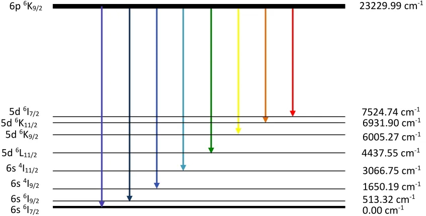
In order to calculate a transition probability a branching fraction is required. A branching fraction indicates the probability for an atom in an excited state to decay via a specific spontaneous emission decay route (one transition) relative to the probability of decaying along all possible decay routes (all allowed transitions.) The sum of all the branching fractions for all the allowed transitions out of an excited state must equal one, as the total probability for decay is one. All transitions do not have equal probability of occurring and thus branching fraction measurements are required in order to determine the “strength” of the various transitions out of an excited state. Put another way, the relative branching fractions determine the number of atoms that will decay via one transition or another in a collection of atoms. Figure 1 shows an energy level diagram for singly-ionized neodymium showing the eight allowed transitions to lower energy levels from the 6p 6_K_9/2_{upper energy level at}

23229.99 cm-1_{. This particular level was studied extensively in this thesis. Each of the}

eight transitions has some probability of occurring determined by the transition branching fractions. Thus for each upper energy level, all branching fractions must be reported. This implies that to make such measurements, all transitions must be observed. Equation 1.1 shows how a branching fraction is defined.

𝛽_𝑗𝑖 = 𝐴𝑗𝑖

∑ 𝐴𝑗𝑖 (1.1)

A branching fraction for a transition from an upper state j to a lower state i, βji,

is equal to the Einstein A-coefficient for spontaneous emission of that transition, Aji,

divided by the sum of all Einstein A-coefficients for transitions exiting the upper energy level and ending in different lower levels, i. The Einstein A-coefficient, Aji,

represents the probability per unit time (s-1_{) that an atom in state}_j_{will decay}

spontaneously to state i. Equation 1.2 shows how a branching fraction may be determined.

𝛽𝑗𝑖 =

𝐼_𝑗𝑖

∑ 𝐼𝑗𝑖 (1.2)

The branching fraction βji of the transition from state j to state i is also equal

(18)

4

observed relative emission intensities from all transitions exiting the upper energy level j and ending in different lower levels i. In this thesis, by measuring all the Iji from

an excited state, I will directly determine the branching fractions βji of all decay

transitions starting in that upper state j. Equation 1.3 shows how the radiative lifetime of the upper state j, which is denoted τj, is related to the Einstein

A-coefficients for spontaneous emission.

𝜏_𝑗−1_{= ∑ 𝐴} 𝑗𝑖 𝑖

(1.3)

A radiative lifetime can be thought of as the time an atom will remain in a given upper energy level before it decays. More accurately, it is the inverse of the sum of the Einstein A-coefficients (which are transition rates) for all the transitions out of an upper energy level. Combing equations 1.1 and 1.3 then gives us Equation 1.4.

𝛽𝑗𝑖

𝜏_𝑗 = 𝐴𝑗𝑖 (1.4)

Therefore, an experimentally determined transition probability for spontaneous emission (Einstein A coefficient) can be determined by dividing an experimentally determined branching fraction with an experimentally measured

0.00 cm-1

513.32 cm-1

1650.19 cm-1

3066.75 cm-1

4437.55 cm-1

6005.27 cm-1

6931.90 cm-1

7524.74 cm-1

23229.99 cm-1

6s 6_I 7/2

6s 6_I 9/2

6s 4_I 9/2

6s 4_I 11/2

5d 6_L 11/2

5d 6_K 9/2

5d 6_K 11/2

5d 6_I 7/2

6p 6_K 9/2

Figure 1.1 Singly-ionized neodymium energy level diagram showing the eight lower

energy levels which have allowed spontaneous emission transitions from the 6p 6_K_9/2

(19)

5

upper state lifetime. In this thesis, only the branching fractions βji will be measured.

We will utilize the experimental lifetimes of others to calculate transition probabilities. In some studies the product gjAji or just gA is reported, where gj is the

multiplicity, or number of degenerate energy levels, of the upper state j. In other studies, and of more use to astronomers, an oscillator strength (gf value or more typically log gf) is reported. An oscillator strength is the number of classical oscillations equivalent to one real atom for a given transition.

𝐴_𝑗𝑖 = 2𝜋𝑒2

𝑚_𝑒𝑐𝜀₀𝜆2

𝑔_𝑖

𝑔_𝑗𝑓𝑗𝑖 (1.5)

Equation 1.5 shows how an Einstein A-coefficient is defined in terms of the oscillator strength, fji, the upper and lower energy levels degeneracies, gj and gi, the

transition wavelength, λ, the mass of the electron, me, the speed of light, c, the electron

charge e, and the permittivity of free space, ε0.

1.2.2 Experimental Determinations of Branching Fractions

(20)

6

ejection and ionization of ions from the cathode material. These ions (from the cathode) become excited and decay to lower energy states. The resulting ion emission, combined with interferometry and FTS, allows the determination of transition probabilities. A list of previous work is included and discussed in more detail in Chapter 6.

The use of laser-induced plasmas for this purpose has been proposed as a relatively new technique for transition probability measurements due to its ability (with limited sample preparation) to quickly and easily highly-excite atoms and ions and thus observe branching fractions on various species all with no change to the experimental setup. With only the change of a solid lanthanide target measurements on multiple lanthanides (including various ionization states, neutral - I, singly-ionized - II, and doubly-ionized - III) can be completed in a time span of a few minutes.

1.3 Laser-Induced Breakdown Spectroscopy

This work will entail the use of laser-induced breakdown spectroscopy (LIBS) to make accurate atomic measurements. LIBS involves the focusing of a high-energy pulsed laser onto a target, which creates a weakly-ionized plasma to act as a source of highly-excited atoms and ions. LIBS rapid production of highly-excited atoms and ions allows for measurement and determination of atomic data. LIBS has just begun to be used for atomic measurements [6]. One of the benefits to using LIBS for atomic measurements is the ease of production of highly-excited atoms which in other techniques is not possible due to the energy required to populate a highly-excited state. A thorough description of LIBS is provided in Chapter 2.

(21)

7

measurement the filters are chosen to only allow light from a transition entering and a transition exiting an upper energy level to pass through. Using single-photon counting devices, photons resulting from the transition entering and exiting the level can be observed. Using fast-timing electronics and pulse analysis, the time between start and stop pulses (photon observations) are measured and the experiment is repeated to determine a radiative lifetime of an excited state under investigation.

1.4 Scope of Thesis

The scope of this work is to improve an existing experimental apparatus and analysis technique to increase the accuracy of our transition probability measurements as well as making new measurements of neutral and doubly-ionized species by optimizing experimental parameters.

In Chapter 2 I discuss laser-induced breakdown spectroscopy theory to provide a better understanding of how atomic measurements may be made on a laser-induced plasma. I will also describe several relevant effects that it is necessary to understand when using a laser-induced plasma for such atomic measurements. In Chapter 3 I discuss the experimental setup and the new components I designed and implemented to improve light collection. In Chapter 4 I discuss experimental parameter optimization to increase observed emission from specific species in the plasma, which results in an improved measurement of emission lines and the observation of previously unobservable emission lines. In Chapter 5 I discuss the data and error analysis of the spectroscopic data for measurement of transition probabilities. In Chapter 6 I report and discuss transition probability measurements made on our laser-induced plasmas. In Chapter 7 I introduce and discuss a new method, laser-induced breakdown spectroscopy – laser-induced fluorescence (LIBS-LIF), for atomic measurements to minimize and alleviate certain problems associated with atomic measurements on laser-induced plasmas. In Chapter 8 I summarize the work presented in this thesis and discuss future work. In Appendix A I list programs used for automated data analysis.

(22)

8

References

[1] Sneden, C., Lawler, J. E., & Cowan, J. J. (2002). Galactic cosmochronometry from radioactive elements in the spectra of very old metal-poor stars. Physica Scripta, 2002(T100), 15.

[2] Wahlgren, G. M. (2002). The lanthanide elements in stellar and laboratory spectra. Physica Scripta, 2002(T100), 22.

[3] Lawler, J. E., Bilty, K. A., & Den Hartog, E. A. (2011). Atomic transition probabilities of Gd I. Journal of Physics B: Atomic, Molecular and Optical Physics, 44(9), 095001.

[4] Biémont, É. (2005). Recent advances and difficulties in oscillator strength determination for rare-earth elements and ions. Physica Scripta, 2005(T119), 55.

[5] Carroll, B. W., & Ostlie, D. A. An introduction to modern astrophysics, 2007. [6] Xu, H. L., Persson, A., Svanberg, S., Blagoev, K., Malcheva, G., Pentchev, V., ... &

(23)

9

CHAPTER 2: Laser-Induced Breakdown Spectroscopy

Laser-induced breakdown spectroscopy (LIBS) is a time-resolved spectroscopy of optical emission from a weakly-ionized (~10%) plasma generated by a high-energy pulsed laser. LIBS can be used as a qualitative and quantitative analysis technique on a variety of substrates (LIBS works equally as well on solids, liquids, and gases) as has been described in great detail in a number of recent authoritative books [1-4]. LIBS can be used for a wide variety of applications ranging from bacterial discrimination to explosive identification by measuring the atomic composition of the material [5, 6]. This chapter will give an introduction to LIBS and discuss some of the key concepts in laser-induced plasma spectroscopy.

2.1 Plasma Production (Nanosecond Laser Regime)

When a high-energy nanosecond laser pulse is incident on a target, it acts to vaporize and atomize the target, followed by ionization and excitation of the created cloud of atoms. I used a Nd:YAG laser with a pulse duration of 10 ns and a wavelength of 1064 nm. Any wavelength could be used for LIBS as long as the wavelength is sufficiently absorbed by the target [1]. A pulsed laser is ideal for LIBS as it provides sufficient energy fluence to cause the breakdown [1] (atomization and liberation of electrons) of the target material. I will only discuss the nanosecond regime for plasma production since it was the only plasma production method used for my thesis (other regimes that exist are femtosecond and picosecond laser plasma production).

(24)

10

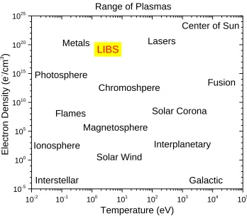
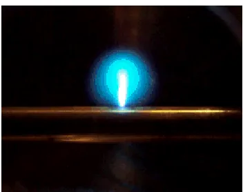
shows the parameters for laser-induced plasmas compared to other common plasmas. Figure 2.2 schematically shows the laser-induced plasma formation process just described. The time from incident laser pulse to ionization of atoms is tens of nanoseconds and the temperature of the plasma at formation can exceed 50,000 K [2]. The plasma is elongated in the direction of the incident laser pulse due to the absorption of the laser pulse as shown in Figure 2.3 which is a photograph taken in our lab. The vaporized atoms travel outwards at supersonic speeds, which results in the formation of a shockwave. Over the first few hundred nanoseconds of plasma evolution, continuum emission dominates and no useful information can be obtained from the light emitted from the plasma. As the plasma cools, electrons recombine with ions and the atoms and ions decay to lower energy states. Ionized and then neutral emission from the ions and atoms in the plasma may be observed over the following

Figure 2.1 Plasma regimes characterized by electron density and temperature with

laser-induced plasmas near the mid-range of temperature and high-end of electron density in comparison to other the other types of plasmas seen in this figure [7].

10-2 10-1 100 101 102 103 104 105 10-5

100 105 1010 1015 1020 1025

Electro

n De

nsity (

e

- /cm 3 )

Temperature (eV) Range of Plasmas

Center of Sun

Interstellar

Lasers Metals

Photosphere

Flames

Ionosphere

Magnetosphere

Solar Wind

Galactic Interplanetary Solar Corona

Fusion Chromoshpere

(25)

11

tens of microseconds. The plasma consists of free electrons, ions, atoms, and molecules in varying ratios depending on the time evolution of the plasma to be discussed in Section 2.2.

Figure 2.3 A laser-induced plasma on a metal target inside a vacuum chamber displaying

the elongation of the plasma in the direction of the incident laser pulse (the laser was incident from above in this picture orientation).

Figure 2.2 A LIBS plasma production schematic. (a) Shows the laser pulse incident on a

target material. The target will absorb the laser energy causing melting, heating and vaporization. (b) The incident laser pulse has now ablated a small portion of the target material and produced a cloud of atoms above the target that will absorb the remaining energy of the laser pulse. (c) The plasma has now formed, it is very hot and dense, and the final energy of the laser pulse is absorbed. A shockwave and continuum emission is produced at formation of the plasma. (d) After a few hundred nanoseconds continuum emission has decreased and element-specific atomic and ionic emission is observed [1].

Material Absorption

In

cid

en

t Las

er

Pu

ls

e

Crater

In

cid

en

t Las

er

P

u

ls

e

Cloud of Atoms

Plasm

a

P

las

m

a

(26)

12

2.2 Plasma Evolution

The plasma is very hot and very dense at its formation and continuum emission dominates for the first few hundred nanoseconds, as previously mentioned. This results in large background emission and no useful information is observed from the plasma. As the plasma begins to cool, background emission decreases and ionic emission can be observed. The ionization states observed as the plasma evolves can be estimated using the Saha-Boltzmann equation (Equation 2.1). This equation characterizes the fraction of atoms in each ionization state as a function of temperature, T, and electron density, Ne, both of which evolve in time. NI,k and NA,j are

the number of atoms per unit volume in the kth and jth energy levels in corresponding ionization states I and A, me is the mass of an electron, kB is the Boltzmann constant,

h is Planck’s constant, gI,k and gA,j are the multiplicity for the kth and jth energy levels

in the I and A ionization states, χZ is the ionization potential, and Ek and Ej are the

energies of the kth and jth levels. A constant Ne of 1024 cm-3 was used to produce a

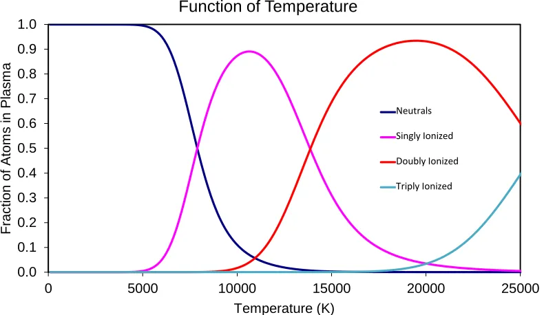
graph that approximated the fraction of atoms in a given ionization state as a function of temperature for the first few ionization states of neodymium (Figure 2.4). This calculation allowed for comparison of our plasma temperature and observed ionization states in various spectra. Changing our observation time after plasma formation allowed us to observe different plasma temperatures and thus compare the observed spectra to Figure 2.4.

𝑁_𝐼,𝑘 𝑁𝐴,𝑗 =

1 𝑁𝑒

2(2𝜋𝑚_𝑒𝑘_𝐵𝑇)3/2

ℎ3

𝑔_𝐼,𝑘 𝑔𝐴,𝑗𝑒𝑥𝑝 [

−(𝜒𝑍+ 𝐸𝑘− 𝐸𝑗)

𝑘𝐵𝑇 ] (2.1)

(27)

13

dominate from 1 to 3 microseconds with a plasma temperature of approximately 12,000 K. At 12,000 K in Figure 2.4 we see singly-ionized species dominate with minimal doubly-ionized and neutral atoms present. This again correlates with what is observed in the red spectrum in Figure 2.5 with the majority of observed emission resulting from Nd II. The plasma continues to cool and electrons recombine with ions to form neutral atoms and neutral emission (from Nd I) increases in the plasma from 3 to 13 microseconds with a plasma temperature of approximately 8,000 K at 3 microseconds. This is again seen in Figure 2.5 in the blue spectrum that contains some Nd II emission and mostly Nd I emission by observing the plasma until 13 microseconds. This correlates with the calculation in Figure 2.4 since 8,000 K is approximately the crossover point at which Nd I becomes the dominant species. At 13 microseconds Nd I must dominate since the plasma is observed to be approximately 4,000 K.

Beyond 13 microseconds emission from the plasma becomes unobservable with our atomic measurement setup. Molecular emission would be observed in most LIBS plasmas from approximately 7 microseconds onwards [2], but due to our plasma consisting of only one lanthanide species and argon gas no molecular emission was observed. An argon gas environment is used for plasma formation to increase ionic and atomic emission by creating a hotter and denser plasma in comparison to air. The increase in emission also results in an increased single-to-noise ratio when ablating targets in argon [2].

2.3 Factors Effecting Plasma Emission

There are key factors that need to be considered when atomic measurements are to be made in a laser-induced plasma. In order to determine the population of atoms in a given energy level the plasma needs to be in local thermodynamic equilibrium (LTE). LTE is an approximation to true thermodynamic equilibrium and allows the plasma to be characterized by a single value of electron density (Ne) and

electron temperature (Te). Knowing these two critical parameters allows one to be

(28)

14

radiation distributions in the plasma [1]. The electron temperature and density also determine Stark effects (such as the broadening or shifting of emission lines), optical thinness, and collisional de-excitation [1], which could affect the measured branching fractions. Since the Ne and Te of the plasma are evolving with time, the plasma needs

to be observed only in conditions of LTE to make atomic measurements.

Emission lines can be Stark-shifted and/or Stark-broadened if the electron density is large. A large electron density results in strong local electric fields and the shifting and splitting of observed energy levels. With a very large electron density broad emission lines are observed that decrease the accuracy of results as well as

0.0 0.1 0.2 0.3 0.4 0.5 0.6 0.7 0.8 0.9 1.0

0 5000 10000 15000 20000 25000

F

rac

ti

on

of

A

tom

s

i

n

P

las

m

a

Temperature (K)

Fraction of Neodymium Atoms in a Given Ionization State as a Function of Temperature

ratio 0

ratio 1

ratio 2

ratio 3

Neutrals

Singly Ionized

Doubly Ionized

Triply Ionized

Figure 2.4 Using the Saha-Boltzmann equation one can see the relative number of

neodymium atoms and ions at different plasma temperatures, which agreed with our observed spectra at various delay times after plasma production. Changing the delay time allowed us to observe different temperatures and thus what ionization state(s) were present in the spectrum. This graph also demonstrates why it is most effective to only observe one ionization state at a time and thus optimize parameters for only that ionization state. The temperature at which certain ionization states are present depends on the electron density of the plasma as well as the ionization energies of the states as seen in Equation 2.1. This graph was calculated using neodymium atomic values and an Ne of 1024

(29)

15

contributing to multiple other problems that will be discussed in Chapter 4 (i.e. the blending of emission lines which renders them unresolvable).

An optically thin plasma is required to make atomic measurements. To be considered “optically thin” all photons emitted from an excited energy level via spontaneous decay must not be reabsorbed by another atom before leaving the plasma. Thus, in an optically thick regime not all photons emitted via spontaneous emission are observed and the resulting measured branching fractions could be incorrect since the absorption of photons (and thus the measured “emission”) is dependent on the transition strength.

Being in a regime where no collisional de-excitation occurs is also imperative. If the ions and atoms are not spontaneously decaying, but are de-exciting due to collisions between atoms, branching fractions cannot be measured, as the observed

Nd III (Black)

Nd II (Red)

Nd I (Blue)

Figure 2.5 An Nd III, Nd II, and Nd I spectrum obtained at various plasma temperatures by

varying the observation time of the plasma. These plasma spectra were not obtained at the same time and have been overlaid and scaled for clarity. The Nd III emission (black) was observed very shortly after plasma formation while the Nd II (red) and the Nd I (blue) spectra were observed at later times. This shows roughly the fraction of each ionization state present at different plasma temperatures and also demonstrates the decrease in plasma temperature with time. This is discussed more in Chapter 4.

Wavelength (nm)

R

el

at

iv

e In

te

ns

it

y (

(30)

16

(31)

17

References

[1] Miziolek, A. W., Palleschi, V., & Schechter, I. (Eds.). (2006). Laser-induced breakdown spectroscopy (LIBS) (pp. 127-136). Cambridge: Cambridge University Press.

[2] Singh, J. P., & Thakur, S. N. (Eds.). (2007). Laser-induced breakdown spectroscopy. Elsevier.

[3] Cremers, D. A., Yueh, F. Y., Singh, J. P., & Zhang, H. (2006). Laser‐Induced Breakdown Spectroscopy, Elemental Analysis. John Wiley & Sons, Ltd. [4] Radziemski, L. J., & Cremers, D. A. (1989). Laser-induced plasmas and

applications.

[5] Cremers, D. A., & Chinni, R. C. (2009). Laser-induced breakdown

spectroscopy—capabilities and limitations. Applied Spectroscopy Reviews, 44(6), 457-506.

[6] Pasquini, C., Cortez, J., Silva, L., & Gonzaga, F. B. (2007). Laser induced breakdown spectroscopy. Journal of the Brazilian Chemical Society, 18(3), 463-512.

(32)

18

CHAPTER 3: Experimental Apparatus

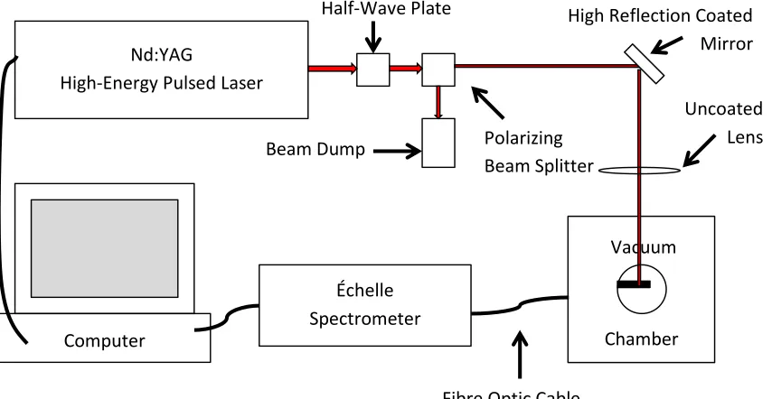
Our laser-induced breakdown spectroscopy setup for atomic measurements consisted of a high-energy pulsed laser, various optical components, vacuum chamber, spectrometer, and computer. This chapter will describe the setup and component design of the LIBS experimental apparatus for atomic measurements. Figure 3.1 shows an overview of the LIBS experimental setup consisting of the aforementioned components to be described in detail in the following sections. This chapter will also discuss an optical parametric oscillator (OPO) that was used for a hyphenated LIBS technique that is discussed in Chapter 7.

3.1 High-Energy Pulsed Laser

A neodymium-doped yttrium aluminum garnet (Nd:YAG) pulsed laser (Quanta Ray LAB-150, Spectra Physics) was used to produce the laser-induced plasma. The Nd:YAG laser has a 10 ns pulse duration, 10 Hz repetition rate, and operates at its fundamental frequency with a wavelength of 1064 nm. The laser outputs a maximum

Figure 3.1 An overview schematic of the experimental setup for our atomic measurements

apparatus. The setup contains a high-energy pulsed infrared laser, energy attenuating optics, directing and focusing optics, vacuum cube, optical fiber, échelle diffraction grating spectrometer, and control computer.

Vacuum

Chamber Échelle

Spectrometer Computer

Half-Wave Plate

Polarizing Beam Splitter Beam Dump

High Reflection Coated Mirror Nd:YAG

High-Energy Pulsed Laser

Fibre Optic Cable

(33)

19

energy of 650 mJ per pulse. This pulse duration and energy results in a large peak power. For our atomic measurements the laser pulse energy is attenuated down to 30 mJ per pulse through the use of a rotatable half-wave plate and polarizing beam splitter (Glan-Taylor calcite polarizer). See Figure 3.2. With a laser pulse energy of 30 mJ focused to a roughly circular spot with a diameter of 100 µm, an irradiance of 1010_W/cm2_{is achieved. This irradiance is in agreement with previously published}

breakdown threshold irradiances [1]. A half-wave plate rotates the polarization of linearly polarized light incident upon it. It has two different indices of refraction along perpendicular directions (fast and slow axes) arising from the crystal lattice structure. The properties of a half-wave plate are such that when the light exits the crystal the polarization component of light parallel to the slow axis is one half wavelength retarded relative to the polarization component of light parallel to the fast axis. By careful choice of the orientation of the crystal the linear polarization of the incident laser pulse can be rotated by any angle through this induced phase shift between the two polarization components of light.

A polarizing beam splitter is placed after the half-wave plate that only transmits the vertical (p-polarized) polarized component of light and reflects the horizontally (s-polarized) polarized component. By rotating the half wave plate appropriately the polarization of the laser light is rotated sufficiently so that only 30 mJ per pulse (as measured by an optical power meter, Coherent FieldMax II) is vertically polarized and thus transmitted through the polarizing beam splitter. The

Figure 3.2 Spectra Physics Quanta Ray high-energy pulsed laser with half-wave plate,

polarizing beam splitter, and power meter.

Half-Wave Plate Polarizing Beam Splitter

(34)

20

beam splitter directs the remaining energy of the laser pulse into a beam dump. The polarization of the beam is insignificant for production of the plasma and is only important in the energy attenuation of the beam. The laser pulse is directed into a vacuum chamber using high-damage threshold 1064 nm high-reflection dielectric-coated mirrors (>99.9% of the 1064 nm light is reflected). The laser light is focused with an uncoated 75 mm diameter plano-convex lens with a focal length of 175 mm. The focused laser light passes through a 1064 nm anti-reflection coated vacuum window into the vacuum chamber and onto the target. A computer, with a fast-pulse generator that runs the spectrometer and analysis software (to be described in Section 3.3), controls the timing and firing of the laser.

3.2 Vacuum Chamber

The target is contained inside a vacuum cube of volume 3500 cm3_{. Each side}

of the vacuum cube has a 6-inch circular ConFlat (CF) vacuum flange with 2.75-inch CF flange openings in the center for optical access (except for the bottom side which has a blank 6-inch flange). See Figure 3.3. As mentioned in Section 3.1, attached to the front of the chamber is a 2.75-inch flange with an AR coated window for transmitting the incident laser light. Attached to the back of the vacuum cube is a Pirani convection module pressure gauge (Kurt J. Lesker 300-series) monitoring the pressure inside the chamber calibrated for nitrogen gas. The pressure is monitored through the voltage required to keep a gold-plated tungsten filament at a constant temperature against thermal cooling by the gas environment. The vacuum chamber was filled with argon gas for increased light emission from the plasma. Since the pressure gauge is calibrated to nitrogen, the displayed pressure was converted to actual pressure using a piecewise function based on manufacture-calibrated specifications.

(35)

21

Argon gas is slowly let into the chamber through a needle valve. With fine control of the shut off valve for the vacuum pump and needle valve for inflow of argon, the pressure is adjustable from 100 mTorr to atmosphere and is stable for hours at a time. Attached to the top of the cube is a vacuum rotational feedthrough with a direct current (DC) motor mounted to the 6-inch flange. The target is screwed onto an 80-pitch screw drive driven by a hexagonal key (which is the DC motor drive shaft) inside the 80-pitch screw, see Figure 3.4. The screw turns within an 80-pitch sleeve

Figure 3.3 The vacuum cube with rotational feedthrough, AR coated window, uncoated

lens, Pirani pressure gauge, vacuum finger, and fiber optic cable.

Rotational Vacuum Feedthrough Pirani Pressure Gauge

Uncoated Lens Vacuum Finger

AR Coated Window

(36)

22

rigidly attached to a support structure inside the chamber. As the motor spins the target rotates and translates linearly, thus the fixed laser spark ablates the target in a helical pattern resulting in a new area of the target ablated with subsequent laser pulses. This is necessary to keep the laser from “drilling” a crater into the target. The vacuum feedthrough flange was mounted on top of the cube with a single 6-inch Viton O-ring for ease of removal when changing targets as well as access into the vacuum cube. The right side of the chamber has a regular 2.75-inch flange window (unused in the experiment) for viewing inside the chamber.

The left side of the vacuum cube has a modified 2.75-inch flange with an inset vacuum finger that extends into the vacuum chamber, see Figure 3.5. I designed this flange/finger for improved light collection. The vacuum finger has a 1-inch diameter stainless steel tube attach to the flange with a quartz window mounted at the end of the tube to allow for positioning of the fibre closer to the plasma. The center of a

2.75-Rotational DC Motor

6-Inch CF Flange

Rigid Support Structure 80-Pitch Screw

Metal Ablation Target 80-Pitch Sleeve

Figure 3.4 A schematic of the vacuum rotational feedthrough and target mounting system.

(37)

23

inch flange flat was bored out to a 1-inch diameter hole and a 1-inch diameter stainless steel tube was vacuum welded to the modified flange. The stainless steel tube protruded three and a half inches into the vacuum chamber from the inside surface of the modified flange. A custom-designed window holder was vacuum welded to the other end of the stainless steel tube. The window was inserted into the window holder and pressed against a rubber O-ring. A cover attached by screws into the end of the tube pressed the window against the O-ring and this formed a vacuum seal around the window. This allowed for cleaning and changing of the window at the end of the vacuum finger. The vacuum finger allowed for improved light collection by moving our optical fibre 9 centimetres closer to the plasma. Light is emitted isotropically from the plasma and therefore intensity drops approximately as one over the distance squared. Moving the optical fibre closer to the plasma allowed for capturing more light from the plasma and increased our sensitivity and accuracy by increasing the signal-to-noise ratio (SNR).

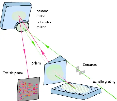
3.3 Light Collection and Analysis

A 1-meter long UV-enhanced optical fibre is attached to an SMA connecter inside a 4-inch length, half-inch diameter tube positioned inside the vacuum finger. This allows the end of the fibre to be located millimetres from the quartz window at the end of the vacuum finger 20 mm from the plasma. The optical fibre is then attached to our échelle diffraction grating spectrometer. In our lab we have two spectrometers: an LLA Instruments ESA 3000 and LTB Aryelle Butterfly. Each

Figure 3.5 Thevacuum finger design schematic with a modified bored out 2.75-inch

CF flange, 1-inch diameter stainless steel tube, and vacuum sealable window holder.

Modified 2.75-inch CF Flange

Stainless Steel Tube

(38)

24

spectrometer has an échelle diffraction grating spectrograph and camera. All data was taken with the ESA 3000 spectrometer, which I will now explain in detail.

The ESA 3000 spectrometer consists of an échelle diffraction grating, dispersing prism, image intensifier, and charge coupled device (CCD). The light from the optical fibre is directed onto the échelle diffracting grating, a reflective surface with equally spaced grooves. The core of the optical fibre (600 micron diameter) acts as the entrance slit of this spectrometer. An échelle diffraction grating is characterized by a low groove density with a high angle of incidence optimized for high diffraction orders. In our échelle orders 29 to 129 are used and all overlap. The diffraction grating gives a 1-dimensional spread of light with longer wavelengths (infrared light up to 780 nm) contained in the lower orders and shorter wavelengths (ultraviolet (UV) light down to 200 nm) contained in the higher orders. The lower orders have a larger angular spread as well as a larger range of wavelengths; this results in decreased spectral resolution at the longer wavelengths. In fact, our spectrometer is optimized for high resolution in the ultraviolet. The manufacturer quotes spectrometer resolution as 0.005 nm at 200 nm and 0.019 nm at 780 nm. A cross-dispersing prism is used to separate the order overlap which results in a 2D spread of light, the 2 dimensions being order (which is also wavelength) and wavelength. The 2-dimensional array of light is then directed using a focusing mirror towards the image intensifier. See Figure 3.6 for the manufacturer-provided schematic of the optical path inside the échelle spectrometer.

(39)

25

produced photons are then detected and recorded by a 2-dimensional 1024 by 1024 array (24 x 24 μm2_{pixel size) of charge-coupled devices (CCD).}

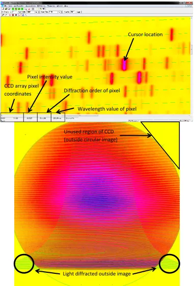
Since the image of the entrance “slit” is circular and the CCD is square, a mapping of a circle to a square needs to be chosen. For optimal resolution in the ultraviolet regime, spectral gaps in the spectrometer resulted from the mapping of the image (circular) to the CCD array (square). At this optimal UV resolution, some light with longer wavelengths is dispersed and diffracted outside the CCD array; these are areas of missed light that we refer to as “spectral gaps,” see Figure 3.7. Mapping could be chosen to direct all light onto the CCD array but this will reduce resolution by increasing the range of wavelengths incident on each CCD pixel. The 2-dimensional

Figure 3.6 Schematic of ouréchelle diffraction grating spectrometer. The incident light is

(40)

26

CCD array pixel intensity values (proportional to incident photons) are the raw data. This 2D picture is known as an échellogram. The CCD array is readout by the computer that performs a spectral calibration to take into account the variation of the imaging systems response with wavelength and then stitches together all the échelle orders to produce a spectrum from the échellogram.

A computer controls the timing of the spectrometer with a fast pulse generator capable of nanosecond accuracy. TTL-pulses are sent from the pulse generator to control the flash-lamp and Q-switch of the high-energy pulsed laser as well as the image intensifier. In a graphical user interface (GUI) a gate delay is set to a desired time after plasma formation for observation. The gate delay sets the time between a TTL-pulse for Q-switch activation of the laser and a TTL-pulse for activation of the image intensifier. A gate width, which determines how long the camera intensifier window is “open” and thus how long the plasma is observed, is also set in the GUI. The nanosecond timing allows for any observation window length to be set anywhere in time. Typical gate delays are between 500 nanoseconds and 10 microseconds with gate widths ranging from 100’s of nanoseconds to 20 microseconds. This timing is shown schematically in Figure 3.8.

3.4 Optical Parametric Oscillator

A second laser system, an optical parametric oscillator (OPO), was used in a hyphenated technique called LIBS-LIF (laser-induced breakdown spectroscopy – laser-induced fluorescence) as described in Chapter 7. An OPO is a high-energy tuneable pulsed laser with a continuously variable wavelength from approximately 400 to 700 nm. The OPO uses a non-linear optical crystal and a laser pump source to produce the range of wavelengths, see Figure 3.9.

(41)

27

Figure 3.7 Top: A zoomed in region of an échellogram displaying various peaks and

diffraction orders shown by the green lines. Bottom: An échellogram of a deuterium-tungsten lamp displaying the mapping of the diffraction pattern (green lines), circular image, and square CCD array.

Light diffracted outside image

(spectral gaps) Unused region of CCD (outside circular image)

Cursor location

CCD array pixel coordinates

Pixel intensity value

(42)

28

The OPO also contains a non-linear crystal. A desired wavelength of light is produced based on the orientation of the incident laser light on the non-linear crystal. The crystal lattice will produce two beams, a signal and idler beam from the incident laser light. The frequency of the signal and idler will sum to the frequency of the pump laser light. The energy output by the OPO is dependent on wavelength and varies in the range from 10 to 100 mJ per pulse. The spectral width of the OPO pulse is 6 wavenumbers, which is sufficient for laser-induced fluorescence. The OPO beam is intrinsically highly divergent and not well collimated. The vertical beam divergence

Figure 3.8 Atiming diagram of the incident laser pulse, plasma evolution, and observation

window characterized by delay time (τd) and gate width (τw).

1 ns 10 ns 100 ns 1 μs 10 μs 100 μs

Laser Pulse

Observation Window

τ

d

τ

w

Elapsed Time After Pulse Incident on Target

Optical

Sig

n

al In

te

n

sit

y

(43)

29

is specified at <25 mrad and the horizontal beam divergence is specified at <1 mrad resulting in an elliptically shaped beam.

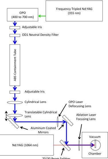
The OPO setup is shown in Figure 3.10. An iris set to a 1 cm beam diameter is placed 10 cm away from the OPO beam exit. This iris is used to block secondary beams exiting from the OPO as well as various reflections. A 1 OD (optical density) neutral-density half-inch circular filter is used to attenuate the beam down to one-tenth its initial energy. The initial OPO energy is much greater than what is required for our experiment as well as near the damage threshold for our optics. The beam is directed one meter down a thermoplastic polymer (ABS) containment tube towards a second iris that is manipulated based on experimental needs.

The beam then passes through a one-dimensional Keplerian telescope with two cylindrical lenses (plano-convex) to reduce the divergence the beam in the vertical direction. The second lens of this telescope was placed on a translation stage so that the lens position can be easily adjustable for optimal collimation of the beam in the far field. The beam was observed 10 metres from the second lens and the second lens was adjusted for optimal beam shape and collimation at this distance. 10 metres is longer than the beam path to the target, which made this distance satisfactory for observation of collimation. The OPO beam diameter is dependent on the focal length of the two lenses used in the Keplerian telescope. The focal length of the first cylindrical lens is 75.6 mm and the focal length of the second cylindrical lens is 110 mm.

(44)

30

OPO beam (at a 45 degree angle of incidence) and transmits 70% of the infrared beam due to the visible-wavelength thin-film coating. The OPO and 1064 nm Nd:YAG beams are aligned collinear using this beam splitter and therefore had a collinear ablation/fluorescence geometry at the plasma. The OPO beam was approximately 1 by 3 mm in size at the plasma location.

(45)

31

Figure 3.10 The LIBS-LIF experimental setup with a frequency tripled Nd:YAG excitation

laser (355 nm), OPO (400 to 700 nm), various optical components, Nd:YAG (1064 nm) ablation laser, and vacuum chamber.

Vacuum

Chamber Frequency Tripled Nd:YAG

(355 nm) OPO

(400 to 700 nm)

AB

S

C

on

tai

n

me

n

t

Tu

b

e

Nd:YAG (1064 nm) Obs

Adjustable Iris

OD1 Neutral Density Filter

Cylindrical Lens

Translatable Cylindrical Lens

Adjustable Iris

Aluminum Coated Mirrors

70/30 Beam Splitter

Ablation Laser Focusing Lens OPO Laser

(46)

32

References

[1] Cremers, D. A., Yueh, F. Y., Singh, J. P., & Zhang, H. (2006). Laser‐Induced Breakdown Spectroscopy, Elemental Analysis. John Wiley & Sons, Ltd.

(47)

33

CHAPTER 4: Experimental Parameter Optimization to

Improve Branching Fraction Accuracy

The majority of the work for my thesis consisted of optimizing experimental parameters to increase the accuracy of the branching fraction measurements as well as allowing the measurement of new, previously unmeasurable branching fractions. Improving the accuracy of the measurements was key since the motivation for the application in astrophysics was to address the problem of inaccurate or nonexistent data [1]. One significant problem with the current technique was the inability to make good measurements of less intense emission lines (small branches). Many less intense emission lines did not have a sufficient signal-to-noise ratio (SNR) and/or signal-to-background ratio (SBR) for accurate measurements. This resulted in a large uncertainty in the measurement of the integrated area under the curve of the peaks. To increase the accuracy of branching fraction measurements, the SNR and SBR were carefully observed as experimental parameters were changed. It was also imperative to verify that the measured branching fractions did not change as the experimental parameters were changed. As well, the lineshape, full width half maximum (FWHM), and overlap of emission lines were key factors in determining the optimal regime in which to make measurements. The measurements obtained from the spectral data were the absolute intensities of the emission lines, which were determined from the integrated area under the curve calculated by the spectrometer software. This is further discussed in Chapter 5.

(48)

34

4.1 Plasma Observation Timing

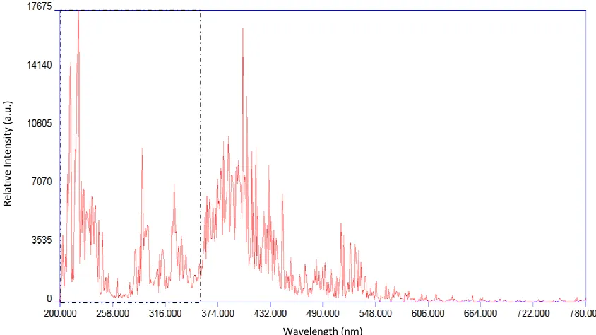
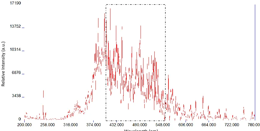
The first parameters studied were the timing for observation of the plasma after its formation (gate delay time) and the length of time to observe the plasma (gate width time). The plasma evolved rapidly in time and the light emitted changed drastically over time which greatly affected the spectra obtained. The plasma was very hot (>50,000 K) and dense at formation and contained many highly excited and energetic atoms. Immediately after its formation no useful information could be obtained as discussed in Chapter 2. After a short delay, once the continuum emission had decreased, doubly-ionized lanthanide species were observed at delay times of 500 ns with a gate width of 500 ns (Figure 4.1). As the plasma cooled, expanded, and became less energetic, singly-ionized species became prevalent and dominated the plasma emission spectrum (Figure 4.2). The emission from the doubly-ionized species was nearly gone by about 1 μs and singly ionized species dominated from 1 to 3 μs. Singly-ionized absolute emission intensities were less intense than the doubly-ionized emission, and the MCP amplification voltage was considerably lower when observing doubly-ionized emission at 500 ns due to the number of photons emitted. After 5 μs the singly-ionized emission had decreased substantially and neutral atom emission had increased. Neutral atom emission dominated the plasma (Figure 4.3) until all emission has ceased or become unobservable, which was approximately 20 μs after formation. The neutral species absolute emission intensity was less intense than the singly-ionized and was therefore the least intense emission. The MCP amplification was raised considerably for neutral emission in comparison to the singly-ionized spectrum to use the full dynamic range of the imaging system. However, this also amplifies the noise. If one spectrum was obtained from 500 ns until 13000 ns after plasma formation and the MCP amplification was set appropriately so as to not saturate the imaging system, neutral emission would be so faint that accurate branching fractions would be impossible (the spectrum would near identical to Figure 4.1).

(49)

35

complex atomic structure and therefore thousands of emission lines (seen in Figure 4.1-.3) that results in a “high density” of emission lines in the spectrum (Figure 4.4). In such areas of “high density” the emission lines begin to overlap resulting in two or more emission lines becoming unresolved and thus unmeasurable as seen in Figure 4.4 between 388.875 and 389.081 nm. Taking data in three different experimental regimes, one for doubly-ionized, one for singly-ionized, and one for neutrals, decreased the overlapping of lines and increased our ability to make measurements on emission lines that would ordinarily be overlapped if we had used only one measurement for all ionization states. By choosing the gate delay time and gate width time appropriately, emission from specific species was maximized while minimizing emission from the others. This reduced the density of emission lines in each spectrum as well as allowed the maximum emission from each ionization state. Frequently, singly-ionized and neutral emission lines would have center wavelengths separated by less than their FWHM resulting in overlapped and unresolved lines. This is shown in Figure 4.5. Since all emission lines from an upper energy level need to be measured in order to calculate branching fractions, having non-overlapping emission lines was vital.

(50)

36

Figure 4.1 A doubly-ionized neodymium LIBS spectrum with a gate delay of 500 ns and

gate width of 500 ns. The majority of the doubly-ionized emission lines are between 200 and 350 nm.

Figure 4.2 A singly-ionized neodymium LIBS spectrum with a gate delay of 1000 ns and

gate width of 1000 ns. The majority of the singly-ionized emission lines are between 350 and 450 nm.

R

el

at

iv

e In

te

ns

it

y (

a.u.)

R

el

at

iv

e In

te

ns

it

y (

a.u.)

Wavelength (nm)

(51)

37

Figure 4.3 A neutral neodymium LIBS spectrum with a gate delay of 3000 ns and gate

width of 10000 ns. The majority of the neutral emission lines are between 370 and 550 nm.

Figure 4.4 A “high density” (of emission lines) region of an Nd II spectrum showing overlap

of multiple emission lines. The three emission lines between 388.875 nm and 389.081 nm (as well as others in this zoomed in region) are completely unresolved and unmeasurable. The x-axis is wavelength in nm and the y-x-axis is emission intensity in arbitrary units.

R

el

at

iv

e In

te

ns

it

y (

a.u.)

R

el

at

iv

e In

te

ns

it

y (

a.u.)

Wavelength (nm)

(52)

38

Figure 4.5 Overlap of emission lines from different ionization states. An Nd II line at 470.655

nm and a Nd I lines at 470.697 nm have overlapped and blended together. Since this spectrum was optimized for Nd II, the Nd I line was small enough that it did not affect the calculation of the Nd II line intensity and thus the Nd II emission line was measureable. The vertical black lines are markers for all Nd emission lines within the view range.

Figure 4.6 The plasma plume at various argon pressures. The laser is vertically incident from

above on a steel target. The plasma is more diffuse at the lower pressure of 0.06 Torr compared to the hotter denser plasma at 1.73 Torr. This trend continues up to atmosphere [2].

96

calculating the standard deviation of 20 identical spectra. To give the reader an idea of the

various plasma densities, pictures of the plume are shown in figure 2.12 at pressures ranging

from 2.3 mbar to 0.08 mbar. The pictures were the result of a common point-and-click Kodak

camera with typical exposure time of tenths of a second. It is clear that at 0.08 mbar the plume is

very spread out and diffuse, whereas at 2.3 mbar the plume looks much brighter and the emission

from the central region is very strong.

Figure 2.12 above shows the plume at various pressures in an argon environment. It is evident that as pressure is decreased in the chamber, the plume becomes more diffuse and less dense.

2.4.2 - Temporal Evolution

The effect that delay time had on measurements of plasma was also investigated. Delay

time is the amount of time between the initial laser pulse and spectroscopic observation of the

plasma. Using a time-resolved spectrometer allows me to vary this time from 10’s of ns after the

laser pulse to 10’s of microseconds. A graph of the observed emission intensity as a function of

delay time for a line of Nd I at 492.453 nm and Nd II at 536.147 nm is shown in Figure 2.13.

1.73 Torr 0.38 Torr 0.30 Torr 0.15 Torr 0.06 Torr

R

el

at

iv

e In

te

ns

it

y (

a.u.)

(53)

39

4.2 Argon Pressure for Plasma Formation

As a LIBS plasma evolves in time it expands and cools. Changing the pressure of the gas surrounding the plasma will change how rapidly or how far the plasma expands and thus is directly related to the thermal evolution of the plasma. This also impacts the observation timing of the plasma as discussed in section 4.1. It is clear from human eye observation of the plasma that pressure has a great effect on the expansion of the plasma as seen in Figure 4.6.

(54)

40

Figure 4.7 An emission line from an Nd II upper energy level at 430.357 nm at two

different pressures. The red spectrum was obtained at a pressure of 760 Torr and the black spectrum was obtained at a pressure of 1 Torr. At atmospheric pressure the neighboring line to 430.357 nm has overlapped and become unresolvable but is clearly separated at 1 Torr.

760 Torr

1 Torr

Figure 4.8 A singly-ionized iron emission line at various pressures. The FWHM does not

decrease below 1 Torr and is limited by the resolution of the imaging system. The narrowest, three overlapping spectra emission lines are at 0.4 Torr (red), 0.7 Torr (black), and 1 Torr (green). The broader three lines are at 10 Torr (orange), 186 Torr (purple), and 513 Torr (blue).

R

el

at

iv

e In

te

ns

it

y (

a.u.)

R

el

at

iv

e In

te

ns

it

y (

a.u.)

Wavelength (nm)

(55)

41

It also needed to be verified that the measured branching fractions did not change with pressure in the chamber. Observed changes of branching fractions could result from the broadening of lines and/or the opacity of the plasma due to the pressure-related changes in size (and electron and ion density) of the plasma. Due to the broadening at higher pressures many smaller emission lines become unmeasurable as the pressure was increased towards atmosphere, which made branching fraction measurements impossible at these pressures. Interestingly, some authors describe atmospheric pressure LIBS measurements for absolute transition strengths [4]. However, it was observed that our branching fractions did not change at lower pressures and agreed with previous measurements performed with the same technique (LIBS) and with ion beam-laser experiments. See Figure 4.10. Since the measurements did not change with pressure and agreed with previous measurements within uncertainty it was also verified that the measurements were taken in a regime of optical thinness and no collisional de-excitation. This will be further discussed in Section 4.3. Therefore, measurements were taken at 1 Torr for optimal achievable emission line width.

4.3 Target Composition

As mentioned in Chapter 2, being in a regime of optical thinness and no collisional de-excitation is imperative to branching fraction measurements so that no photons are reabsorbed by the plasma and all energy levels have spontaneously decayed. Optical thickness and collisional de-excitation could result from a plasma that is too dense and too hot. Thus, the number of atoms or ions in the plasma (defined as Nion, the plasma ion density) has a large role in determining the opacity of the

plasma and the rate of collisional de-excitation. To reliably change Nion by