A Method for Classifying Driver Performance

(1)

University of Windsor University of Windsor

Scholarship at UWindsor

Electronic Theses and Dissertations Theses, Dissertations, and Major Papers

2014

A Method for Classifying Driver Performance

Ishika Zonina Towfic

University of Windsor

Follow this and additional works at: https://scholar.uwindsor.ca/etd

Recommended Citation Recommended Citation

Towfic, Ishika Zonina, "A Method for Classifying Driver Performance" (2014). Electronic Theses and Dissertations. 5164.

https://scholar.uwindsor.ca/etd/5164

This online database contains the full-text of PhD dissertations and Masters’ theses of University of Windsor students from 1954 forward. These documents are made available for personal study and research purposes only, in accordance with the Canadian Copyright Act and the Creative Commons license—CC BY-NC-ND (Attribution, Non-Commercial, No Derivative Works). Under this license, works must always be attributed to the copyright holder (original author), cannot be used for any commercial purposes, and may not be altered. Any other use would require the permission of the copyright holder. Students may inquire about withdrawing their dissertation and/or thesis from this database. For additional inquiries, please contact the repository administrator via email

(2)

A Method for Classifying Driver Performance

By

Ishika Zonina Towfic

A Thesis

Submitted to the Faculty of Graduate Studies

through the Department of Mechanical, Automotive, and Materials Engineering in Partial Fulfillment of the Requirements for

the Degree of Master of Applied Science at the University of Windsor

Windsor, Ontario, Canada

2014

(3)

A Method for Classifying Driver Performance

by

Ishika Zonina Towfic

APPROVED BY:

______________________________________________ Dr. C. Lee

Department of Civil and Environmental Engineering

______________________________________________ Dr. B. Minaker

Department of Mechanical, Automotive, and Materials Engineering

______________________________________________ Dr. J. Johrendt, Advisor

Department of Mechanical, Automotive, and Materials Engineering

(4)

iii

DECLARATION OF ORIGINALITY

I hereby certify that I am the sole author of this thesis and that no part of this

thesis has been published or submitted for publication.

I certify that, to the best of my knowledge, my thesis does not infringe upon anyone’s copyright nor violate any proprietary rights and that any ideas, techniques,

quotations, or any other material from the work of other people included in my

thesis, published or otherwise, are fully acknowledged in accordance with the

standard referencing practices. Furthermore, to the extent that I have included

copyrighted material that surpasses the bounds of fair dealing within the meaning of

the Canada Copyright Act, I certify that I have obtained a written permission from

the copyright owner(s) to include such material(s) in my thesis and have included

copies of such copyright clearances to my appendix.

I declare that this is a true copy of my thesis, including any final revisions,

as approved by my thesis committee and the Graduate Studies office, and that this

thesis has not been submitted for a higher degree to any other University or

(5)

iv

ABSTRACT

Driving performance can be directly related to the driver behaviour in terms

of the mental workload and risk perception. No generally accepted model or system

exists that can model the driving task or driver performance in a comprehensive

manner. The purpose of this research is to develop a methodology using a series of

modelling techniques to evaluate driving performance under naturalistic driving

contexts. Exploratory statistical techniques and artificial neural network have been

used as the backbone of the work presented in this thesis to determine and classify

driver performance in different categories by identifying underlying natural sub-sets

in the driving data set. A safe and experienced driver should possess the knowledge

and the experience about his/her driving skills along with an acute awareness of the

surrounding driving environment. The methodology proposed in this thesis can be

used for various applications including evaluation of driving performance of

(6)

v

DEDICATION

To my loving parents, Dina and Towfic,

For their unwavering support, unconditional love,

And continuous encouragement.

(7)

vi

ACKNOWLEDGEMENTS

There are a number of people without whom this journey would have not

been possible. I am forever indebted to them. I would also like to thank the AUTO21

Network of Centres of Excellence for their funding support for this research.

Foremost, I would like to express my deepest gratitude and appreciation for

my supervisor, Dr. Johrendt, for her patience, knowledge, motivation, technical

guidance, and kindness. I consider myself extremely fortunate to have her as my

mentor and I am very thankful to her for believing in me. I would also like to thank

my committee members, Dr. Minaker and Dr. Lee, for their technical guidance and

support throughout the course of this research. Dr. Minaker has always offered me

valuable advice, and Dr. Lee has helped me understand and learn the importance of

statistical techniques for conducting this research. Much of what I have learnt and achieved during my Master’s program is due to my supervisor and my committee

members.

I would also like to take this opportunity to thank the Safety Ambulance

Monitoring Unit (SAMU) research team and Université Laval for providing me with

the resources for successfully conducting this research.

There are some very special people that I would like to acknowledge and express my sincerest gratitude. I would like to thank my sisters, Adiba and Tasnuva, for

believing in me and being there for me through thick and thin. I would like to

specially thank my partner, Luv, for his patience and understanding. He has always

kindly lent me his ears and patiently listened to all my worries and troubles even

when it made no sense. I am very grateful for his support and his advice. He has

been an integral part of my journey.

“I have no special talents. I am only passionately curious.”

(8)

vii

LIST OF FIGURES

Figure 1.1: Research Methodology ... 3

Figure 2.1: Comprehensive Overview of a Sample Driver Model ... 6

Figure 3.1: Hierarchical Agglomerative Clustering Method Overview ... 17

Figure 3.2: Hierarchical Agglomerative Clustering using Ward’s method ... 19

Figure 3.3: Sample Dendogram to Visualize Clusters ... 19

Figure 3.4: Sample Scree Plot to Determine Number of Factors ... 24

Figure 4.1: Feedforward MLP Network Architecture ... 26

Figure 4.2: Processing Unit... 27

Figure 5.1: Visual Information from Internal and External Environment of the Vehicle Synchronized and Fused Together ... 37

Figure 5.2: ECEF Coordinates ... 38

Figure 5.3: (a) Raw Signal from Latitude Channel (b) Latitude Channel after “Zero” Correction ... 39

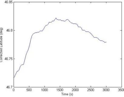
Figure 5.4: Example of a Final Corrected Latitude Channel obtained from raw GPS data ... 40

Figure 5.5: Speed Profile for a Prius Test Drive ... 41

Figure 5.6: Comparison between Speed and Acceleration Profile of a Prius Test Drive (a) Speed Profile (b) Acceleration ... 42

Figure 5.7: Total Distance Travelled for a Prius Test Drive ... 43

Figure 6.1: Dendogram of Driving Data Set for Initial Cluster Analysis ... 49

Figure 6.2: Evaluation of Optimal Number of Clusters using C-H Criterion ... 51

Figure 6.3: Evaluation of Optimal Number of Clusters using Gap Criterion ... 52

Figure 6.4: Dendogram Showing Assignment of Data Set in to Four Classes ... 54

Figure 6.5: Neural Network Architecture for Classifying Driver Performance ... 57

Figure 6.6: ANN Performance Curves for Training, Validation, and Testing ... 59

Figure 6.7: Error Histogram for Designed ANN Network ... 60

Figure 6.8: Confusion Matrix for Driver Performance Classification using ANN. 62 Figure 7.1: Scree Plot for Determining the Number of Factors for Factor Model . 67 Figure 7.2: Classification of Driver Performance based on Factor Model ... 71

(13)

xii

LIST OF APPENDICES

Appendix A: Driving Data Set ... 80

Appendix B: Cluster Analysis Results ... 82

Appendix C: ANN Results ... 84

(14)

xiii

LIST OF ABBREVIATIONS/NOMENCLATURE

3D Three dimensional

AANN Auto Associative Neural Networks

ANN Artificial Neural Networks

ANOVA Analysis of Variance

BSLM Boosting Sequential Labelling Method

C-H Calinski and Harabasz Criterion for determining Optimal Number of

Clusters

ECEF Earth Centered, Earth Fixed Coordinate System

EPS Environmental Perceptual System

GADGET Guarding Automobile Drivers through Guidance Education and

Technology

GPS Global Positioning System

GRAME Research Group in Motion Analysis and Ergonomics

LM Levenberg Marquardt Training Algorithm for ANN

LPA Linear Prediction Analysis

MATLAB Numerical Computing and Simulation Software

Minitab Statistical Software Package

MLP Multi-Layer Perceptron

(15)

xiv

LIST OF SYMBOLS

𝑅2 Proportion of variation by a cluster

𝑆𝑆𝐵 Between cluster variance

𝑆𝑆_{𝐸𝑟𝑟𝑜𝑟} Error sum of squares

𝑆𝑆_{𝑇𝑜𝑡𝑎𝑙} Total sum of squares

𝑆𝑆𝑊 Within cluster variance

𝑉₁₀ Percentage of Test Drive where Vehicle Speed Exceeds 10% of

the Posted Speed Limit

𝑉𝑟𝑒𝑠 Resultant vehicle speed in km/h

𝑋̅ Sample mean

𝑥_𝑠𝑡𝑑 Standardized value

𝜎𝑥 Sample standard deviation

𝜎𝑥2 Variance

b Bias value for ANN

C Variance-covariance matrix

d Euclidean distance

der Sum of derivatives of error with respect to the ANN inputs

dist Haversine distance in km

E Error between actual and predicted values

I Identity matrix

L Factor loading matrix

n Number of observations in data set

r Sample Pearson correlation coefficient

RD Residual matrix

u Weighted input

v Eigenvector corresponding to eigenvalue λ

w ANN weight

x, y Variables

(16)

xv

α Damping factor

β Factor loading

λ Eigenvalue

𝑎 Vehicle acceleration

(17)

1

CHAPTER 1 INTRODUCTION

1.1 Research Background

Driving is a complex task that requires the driver to employ a wide range of skills

in order to interact with a complex environment, while simultaneously managing different

driving task demands. The driving task can be considered as the interaction between

various vehicle, driver, and environment characteristics. Nowadays, the magnitude of

information available to drivers through various technological systems and advancements

is simply overwhelming. Each individual driver is unique and thus, their level of

performance greatly relies on their driving behaviour through successful processing of

available information. Every driver has a different perception of acceptable risk levels.

These risk levels are subjective in nature and might be influenced by driver age, gender,

lifestyle, social background, etc., which in turn can dictate the driver performance to a

certain extent. A good driver must therefore possess an adequate level of mental and

physical skills to control the vehicle within the environment that they are expected to

function.

No generally accepted model or system exists that can model the driving task or

driver performance in a comprehensive manner. Driving performance can be directly

related to the driver behaviour in terms of the mental work load and risk perception. The

driver can choose to follow different strategies for a given risky scenario by adjusting the

various driving parameters (e.g. choice of vehicle speed) to constantly adjust the perceived

level of risk to an acceptable value. Moreover, there is no standard set of variables defined

that can be used to develop a comprehensive model encompassing driver performance and

behaviour. The nature of data sets available for analysis varies greatly amongst research

groups since each research group develops driver models tailored to their research needs.

Extensive research has been conducted to understand the reasons leading to

roadway collision events and as such, drivers have been identified as one of the major

(18)

2

demands and levels of interaction or attention required by the driver. According to Transport Canada’s National Collision Database (NCDB), 73% of recorded injury

collisions in 2010 occurred in urban areas, which includes metropolitan streets and

residential areas [1]. Reducing the number of collisions that lead to such events are of key

interest to policy makers around the world. Any such traffic event is the interaction between

the driver, vehicle, and the road. The work done for this thesis involves the use of factors

involved with the vehicle and the road to help identify an evaluation criteria for driver

performance. It is very important to understand and classify driving behaviour under

different categories based on driving performance and associated levels of risk involved.

Such analysis is also very important in understanding and identifying factors that can lead

to risky driving scenarios. The work presented in this thesis can have a wide range of

applications for developing a better understating of the underlying characteristics inherent

to the driving task.

1.2 Research Objectives

A safe and experienced driver should possess the knowledge and the experience

about their driving skills along with an acute awareness of the surrounding driving

environment. However, it is very challenging to objectify and quantify such phenomena

mathematically, based on naturalistic driving data. Often collision scenarios are a result of

driver errors, such as errors in risk perception, driving distractions, etc. Therefore, there is

a need to identify possible factors and scenarios contributing to risky driving behaviour so

that mitigating solutions (e.g. tailored driver training modules) can be further developed to

help prevent risky driving events or collisions.

The purpose of this research is to develop a methodology using a series of

modelling techniques to evaluate driving performance under naturalistic driving contexts,

as presented in Figure 1.1. The methodology was developed using an iterative approach

where every step was verified to ensure accurate model results. This thesis proposes a

classification model based on driver performance that is indicative of the task demand and

risk perception of the driver. In particular, the presented work analyzes the driving

(19)

3

The objective is develop a driver classification model, using artificial neural networks

(ANN), that can classify driver performance using different classes or categories.

Figure 1.1: Research Methodology

Neural network is a very powerful mathematical tool that can determine, predict,

and classify complex non-linear relationships without any prior assumptions. Based on

analysis of a driving data set, the proposed work will attempt to determine the relationship

between the driver performance and the associated risk factors using ANNs and statistical

methods. Statistical modelling techniques will be used extensively used throughout this

thesis to determine and interpret the natural subsets within the driving data set. Emphasis

will also be placed on data processing techniques for tackling complex data sets containing

quantitative information. In particular, the variables presented in this thesis assume

continuous numerical values. Determining associated trends in a given data set is very

important for building successful models using ANNs. Furthermore, the developed model

will be analyzed to determine how individual input parameters affect individual outcomes

of the model, by performing a sensitivity analysis. It should be realized that the proposed

framework developed in the following thesis is based on information available in the data

set. It serves as a guideline and provides an overview of the methodology that will be

implemented to model driver performance, which can be used for various applications.

1.3 Research Applications

Apart from evaluating driving performance under regular driving scenarios, the

work done for this thesis can also be extended to include various other purposes. One such

Data Collection

Data Processing

Outlier Detection & Standardization

Unsupervised Classification

ANN Classification

Model

Factor Analysis for

(20)

4

application is the use of such analysis and modelling techniques for evaluating the driving

performance of emergency services such as ambulances. Recently, there has been growing

concern due to the increased number of ambulance collisions, which can cause serious

injuries to occupants and cause extensive damage to expensive emergency vehicles. For

instance, over 370 ambulance collisions were reported in Quebec City alone in the past five

years [2]. Research indicates that ambulance drivers are one of the most important factors

influencing ambulance collisions. Thus, it is very important to understand individual driver

behaviour and characteristics that can lead to risky behaviours such as speeding and

overtaking other vehicles. Although driving an ambulance in emergency situations will be

different from regular driving conditions, similar methodology and modelling procedures

can be followed to develop an evaluation tool for driver performance. An emergency

situation can be described as a scenario where an ambulance needs to respond immediately

to an emergency call within a specific time frame. It is a dangerous activity that involves

very risky and hazardous situations. The driver is often required to make immediate

decisions based on the available information at that instant. Such analysis will greatly assist

in understanding ambulance collisions and will help in decreasing the number of

ambulance collisions in the future. A similar methodology can also be implemented for

evaluating drivers for effective fleet management.

The work presented in this thesis can be applied to evaluate the performance of

elderly drivers. The age structure of the Canadian population demographics is changing,

with a significant proportion of the population falling under the age group of 65+ years.

Moreover, elderly drivers have a higher risk of being involved in vehicle collisions.

Although aging affects every individual in a different manner; driving skills, in general,

gradually deteriorate due to an increase in reflex or response times. Instead of deciding

arbitrarily to restrict the driving capabilities of an elderly driver, a tool can be developed

to evaluate the performance using a similar methodology to the one outlined in this thesis.

Such a tool will help in developing a quantitative measure for decisions with respect to driving restrictions. This tool in turn can have a positive impact on the quality of life for

(21)

5

CHAPTER 2 LITERATURE REVIEW

A driver performance classification model can serve as the foundation for

understanding driver characteristics and performance that lead to vehicle collisions. Driver

modelling is an ongoing research topic and there exist various models that address various

aspects of driver performance and behaviour. However, a generally acceptable framework

is not available that encompasses all the behavioural effects of a driver that can

comprehensively describe the driving task. Limited research has been conducted in this

area using exploratory statistical methods combined with neural networks. This chapter

highlights some of the important work conducted in this field of research. The knowledge

learnt from previous literature served as a guideline for developing the classification model

for this thesis. The chapter is divided into two sections. The first section introduces some

key theoretical models that have served as the foundation for driver models. The second

section of the chapter presents some relevant work conducted in developing a mathematical

model using the knowledge gained from the theoretical models.

2.1 Theoretical Models

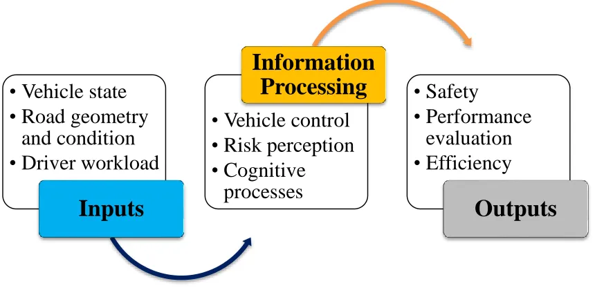
A comprehensive way of developing a driver model can be viewed as a combination

of three major elements: inputs, information processing or behaviour, and outputs [3]

(Figure 2.1). These parameters can be used to determine measures of effectiveness, or to

evaluate driver performance. According to researchers, the occurrence of vehicle collisions

can be reduced significantly if technology were available to detect the driver’s potential

for risky behaviour. If a technology existed that could identify individual driver

characteristics responsible for poor driving performance, it would allow for the

minimization of driver errors (through development of tailed training programs or

advanced vehicle assistance systems), which could play a key role in automotive safety

improvement. Based on Wilde’s risk homeostasis theory, drivers attempt to maintain a

target level of risk per unit time. If the driver is provided with additional safety measures,

the driver will exhibit more risky behaviour to compensate and return to the target level of

risk [3]. Every individual driver has a different level of risk perception; hence, it is very

(22)

6

categorized in different levels, a more comprehensive model for performance evaluation

could be developed. One of the major drawbacks of such theories pertaining to driver

modelling is that they only explain the factors and motivations affecting the driver

behaviour without describing the process involved in determining such behavioural

characteristics. Also, such models cannot quantify factors associated with risk levels which

can be further utilized to develop a mathematical model.

Figure 2.1: Comprehensive Overview of a Sample Driver Model

One of the most popular models for driver behaviour is Michon’s Hierarchical

Control Model [4]. Michon proposed a simple two way classification model for describing driving behaviour. This one dimensional model is appropriate for distinguishing behaviour

using a simple input-output oriented model and internal state models. The second

dimension differentiates between functional and taxonomic models, where model

components may or may not interact with each other [4]. His model was further subdivided

to show that there are three major factors involved in driver decision making: strategy,

maneuvering/tactics, and control [4]. Michon’s driver behavioural model has served as the

basis of various studies over the years in an attempt to develop an effective driver model.

For the purpose of this research, more emphasis will be given to the maneuvering/tactical

• Vehicle state

• Road geometry

and condition

• Driver workload

Inputs

• Vehicle control

• Risk perception

• Cognitive

processes

Information

Processing

_{• Safety}

• Performance

evaluation

• Efficiency

(23)

7

and control levels of the model, since they are associated with the maneuver execution and

decision making processes of the driver. The maneuvering or tactical level is primarily associated with the driver’s interaction with the traffic environment, where the driver’s

actions related to vehicle maneuvering are dependent on his/her level of expertise and

interaction with the surrounding environment.

Another notable model that has been extensively used in the literature is the

Guarding Automobile Drivers through Guidance Education and Technology (GADGET)

matrix [3]. The GADGET matrix was initially developed to assess and structure post

license driver education in the European Union. The GADGET matrix is also based on Michon’s driver model and consists of four categories for describing driver behaviour –

goals for life and skills for living, driving goals and context, mastery of traffic situations,

and vehicle manoeuvering [3]. The levels or cells of the GADGET matrix are not mutually

exclusive due to the inherent complexity of the driving task. It is possible that some

subtasks might be conducted at different levels simultaneously (e.g. speed control,

accelerating, braking, etc.). This model is very important since various driving safety laws

and regulations in Europe and United States were developed based on the findings from

this particular research. For instance, the GADGET matrix was used as the base for

developing key driver competencies, which were then integrated into the driver (category

B) education program in the European Union.

Overall, the driver uses cognitive, perceptual, and motor abilities to successfully

carry out the driving task. Driving can therefore be described as a hierarchy of navigation,

guidance, and control conducted simultaneously with visual search, recognition, and

monitoring operations [5]. Thus based on the theoretical models and assumptions for risk

perception, a comprehensive driver model that can relate the driver performance,

capability, and behaviour to the level of associated risk can be proposed using the following

five categories – attitudes/personality, experience, driver state, task demand/workload, and

(24)

8

2.2 Mathematical Models

Various concepts and theories regarding driver behaviour were explored in Section

2.1. Researchers have used knowledge based on these theories and developed mathematical

models for determining driver behaviour and performance. One of the most important

factors to consider when attempting to develop driver behaviour models is the vehicle

speed. Aarts and van Schagen [6] have highlighted the importance of vehicle speed on road

and traffic safety. According to their research, speed not only affects the severity of a

vehicle collision, but also increases the risk of being in a collision event. The authors

conducted an extensive review of empirical studies relating vehicle speed and the risk of

collision. Based on their review of previous literature, they found that the risk of being

involved in a collision event is higher for vehicles driving in “minor” or urban roadways

when compared to rural or “major” roadways [6]. The authors have also inferred that a

higher average speed in urban or minor roadways leads to a higher risk of crash. These

observations are very important for the purpose of this research because speed was

recorded during the data collection process. Moreover, only the driving data from urban

and residential roadways were selected for modelling the driving performance.

Othman et al. [7], conducted a study on driver behaviour and obtained data from a

driving simulator using a predetermined computer simulated driving course. In order to

extract relevant data from the raw data set, the authors used a linear prediction analysis

(LPA) technique to extract relevant features that could best describe the driver operation

behaviour [7]. Through LPA techniques, parameters were identified using local data sets.

These parameters were used as feature vectors of the driving operation. Feature vectors

contain sets of numerical features that can help describe a particular scenario or object.

Using Auto Associative Neural Networks (AANN), Othman et al. performed an identity

mapping of the feature vectors for each driver and tested the capabilities of the developed

network using sets of features from the same and different drivers. The model was

primarily developed to identify the driver performance; the proposed method had an overall accuracy of 81.70% [7]. Pedal position, speed, and acceleration were used as the input

parameters for the analysis. The model of each driver essentially captured the distribution

of features of that driver, and the overall performance of the model was evaluated through

(25)

9

that it is challenging to interpret the results since it only helps to identify driving patterns;

it does not provide information regarding whether the driving performance is satisfactory

or not.

Constantinescu, Marinoiu, and Vladoiu [8] also investigated the driving styles of

various drivers by classifying the drivers based on their “risk proneness” to group drivers

according to their behaviours. The authors used exploratory statistical methods to identify

the groups of driving styles based on data collected from an in-house built GPS system.

However, the work was only limited to providing some description for each group

identified from the set of experimental results. No attempt was made to develop a

mathematical model to determine the relationship between each set of identified group and

the individual driving parameters.

Another interesting technique was presented by Macadam et al. [9], where the

driver behaviour was classified under five different categories using range and range rates

of longitudinal closures. The data was trained and classified using ANNs. Once the network

was developed, an aggressivity index was defined to reflect the frequency or willingness

of a particular driver to overtake and pass other vehicles [9]. The numbering system,

combined with the age of the drivers, revealed the associated trends and patterns of

behaviour observed in different age groups. However, when a similar technique was

applied to represent the longitudinal control behaviour associated with closing-in and

tracking of a preceding vehicle, the technique did not yield favourable results. One possible

explanation of not obtaining favourable results could be due to the limited number of input

parameters for the ANN network. Since driving behaviour is affected by other road and

environment characteristics, the network could be trained using a different set of

parameters in order to be able classify and predict driver behaviour.

Apart from the use of ANNs, various driver models exist which utilize the concepts

of control theory, vehicle dynamics, fuzzy logic, and genetic algorithms. Models developed

using vehicle dynamics and control theory are very complex in nature and require several prior assumptions. An example is the model proposed by Sharp, Casanova, and Symonds

(26)

10

control theory. It should be noted that the proposed model is non-linear in nature and the

driver model is joined to the vehicle dynamics model to demonstrate the path tracking

performance [10]. The developed model requires priori assumptions and the availability of

a large number of parameters to satisfy the mathematical expressions. The model

demonstrates reliable results but is highly dependent on the assumptions made during the

development of the model. One advantage of using neural networks to model such

behaviour is that no prior assumptions are required, and results may be achieved using a

smaller set of input parameters.

Another example of such a model is the one presented by Raksincharoensak et al.

[11] for modelling naturalistic driving behaviour in traffic scenarios. The authors use a

combined driver behaviour model using a state transition feature. The driver behaviour

model was essentially based on longitudinal vehicle dynamics with a particular focus on

vehicle accelerations and braking. The longitudinal driver model was further categorised

into five driving states from a viewpoint of active safety [11]. The framework of the work

was based on a non-generative method known as the Boosting Sequential Labelling

Method (BSLM) which was used to train the model for driver behaviour recognition. Using

BSLM, the conditional probability was calculated to determine the relationship between

the sensor data and the driving states. Similar to the concept of ANNs, the described

technique (BSLM) is a statistical machine learning technique for real time driver state

recognition. Using such method, varying levels of accuracies were obtained for the five

driving states. A lower accuracy (73%) was observed when determining the driver braking

behaviour. Moreover, the mode results deviate significantly when the training data set for

the algorithm is altered [11], thus showing some inconsistencies in the model.

On the contrary, neural networks have been particularly successful in the field of

driver behaviour modelling since they are able to capture various driving characteristics

through an iterative training process along with iterative parameter adjustments to obtain

the desired results. One of the major challenges for neural networks is to find a method to interpret the final results. Often it can be challenging to determine the relationship between

(27)

11

The literature presented in this chapter has demonstrated the wide range of

techniques and applications of driver behaviour and performance modelling. The variables

considered for analysis were different for each study. Moreover, the level of detailed

information available on the driver-vehicle-environment varies greatly along with the

experimental setup. It is thus often challenging to summarize a set of variables that can

provide a comprehensive overview of driver behaviour. The work conducted for this thesis

utilizes variables (e.g. speed, position, etc.) that can be recorded and obtained in a

straightforward manner to determine the various driving characteristics under naturalistic

(28)

12

CHAPTER 3 STATISTICAL METHODS

The following chapter presents an overview of core statistical concepts relevant to

this work’s analysis of driver performance. Often, such analysis involves

multi-dimensional data with three or more variables. Thus, it is sometimes challenging to

interpret and analyze data in higher dimensions. The chapter begins with an introduction

to mathematical concepts that be will utilized for different statistical modelling techniques.

Two analysis techniques will be introduced in this chapter – cluster analysis and factor

analysis. Cluster analysis is a widely used technique for exploratory data mining and

pattern recognition tasks, amongst many others. Factor analysis is then presented as a

dimension reduction technique to model a given multivariate data set, with minimal loss of

information. The analyses techniques presented in this chapter will be used for the research

presented. The techniques will provide insight into the structure of the data set and help

reduce the complexity of the data by identifying factors that are of key importance for the

developed model.

3.1 Background Mathematics

This section attempts to provide some common mathematical terminology that will

be required to understand the different statistical techniques presented throughout this

thesis. This section is divided into two different parts – statistical concepts and matrix

algebra concepts. Before proceeding, a multivariate data set will be described that will form

the basis of all analysis and techniques mentioned henceforth.

Multivariate Data

Statistical analysis is based on observations and variables. A variable, for the

purpose of this thesis, is described as a unique character or quantity that is measured for

analysis (e.g. vehicle velocity, distance travelled, etc.). Similarly, an observation is defined

as a set of variables or measurements that describes a particular scenario or case. Thus, a

multivariate data set is considered as a data set where two or more variables of interest are

(29)

13

sections are for a sample data set of interest. A sample data set is a subset of the entire

population, which encompasses all possible scenarios or cases.

3.1.1 Statistical Concepts

Some basic statistical measures and computations are presented in this section that

will help to analyze and explore the relationships between different observations and

variables in a given data set.

Sample Mean

The mean or average value of a given variable, 𝑋̅, in a sample data set can be

computed using Equation 1.

𝑆𝑎𝑚𝑝𝑙𝑒 𝑚𝑒𝑎𝑛, 𝑋̅ = ∑𝑥𝑖 𝑛

𝑛

𝑖=1

(1)

where, xi = ith_{observation of variable}_x_,

n = number of observations present in the data set

Sample Standard Deviation and Variance

The standard deviation, 𝜎_𝑥, and variance, 𝜎_𝑥2_{, provide a measure of the spread or}

dispersion of a given variable from its mean value and can be computed using Equations 2

and 3.

𝑆𝑎𝑚𝑝𝑙𝑒 𝑠𝑡𝑎𝑛𝑑𝑎𝑟𝑑 𝑑𝑒𝑣𝑖𝑎𝑡𝑖𝑜𝑛, 𝜎𝑥= √

∑𝑛_𝑖=1(𝑥_𝑖−𝑋̅)2

𝑛 − 1 (2)

𝑉𝑎𝑟𝑖𝑎𝑛𝑐𝑒, 𝜎𝑥2 =

∑𝑛𝑖=1(𝑥𝑖 −𝑋̅)2

𝑛 − 1 (3)

Covariance

Covariance is a statistical measure of the variance between two given variables, x

and y. The covariance can be computed using Equation 4.

𝑐𝑜𝑣(𝑥, 𝑦) = ∑ (𝑥𝑖−

𝑛

𝑖=1 𝑋̅)(𝑦𝑖− 𝑌)̅̅̅

𝑛 − 1 (4)

The sign of the covariance is of particular importance in determining the

relationship between two different variables. A positive sign indicates that the magnitudes

(30)

14

indicates that the magnitude of the first variable increases while the magnitude of the other

variable decreases. If the covariance value is zero, it indicates that the two variables are

independent, i.e. their magnitudes are not dependent on each other.

For a multivariate data set consisting of more than two variables, a covariance

matrix can be formed which contains all the possible covariance values between the

different variables in a data set. A general expression of a covariance matrix, C, of three

variables (x, y, and z) can be presented as follows:

𝐶 = (

𝑐𝑜𝑣(𝑥, 𝑥) 𝑐𝑜𝑣(𝑥, 𝑦) 𝑐𝑜𝑣(𝑥. 𝑧)

𝑐𝑜𝑣(𝑦, 𝑥) 𝑐𝑜𝑣(𝑦, 𝑦) 𝑐𝑜𝑣(𝑧, 𝑧)

𝑐𝑜𝑣(𝑧, 𝑥) 𝑐𝑜𝑣(𝑧, 𝑦) 𝑐𝑜𝑣(𝑧, 𝑧)

) (5)

It is important to note that the diagonal of matrix C is the variance of each individual

variable itself. Thus, C will also be referred to as the variance covariance matrix. Also, it

should be noted that the matrix, C, is symmetrical along the diagonal with cov(x, y) =cov(y,

x).

Correlation

Correlation is another important statistical measure of dependence between two

given variables. The sample Pearson correlation coefficient, r, is used to determine the

correlation coefficient between variables, as expressed in Equation 6.

𝑟 = 1

𝑛 − 1 ∑(

𝑥𝑖 − 𝑋̅ 𝜎𝑥 )(𝑦𝑖− 𝑌̅ 𝜎𝑦 ) 𝑛 𝑖=1 (6)

An r value of +1 indicates a perfectly positive correlation, while a value of -1 indicates a

perfectly negative correlation between the x and y variables under consideration. An r value

of zero indicates that the values are independent of each other. In a similar manner as the

variance covariance matrix, a correlation matrix can also be formed for a multivariate data

set consisting of more than two variables.

3.1.2 Matrix Algebra Concepts

The aim of this section is to provide some important background, pertinent to

matrix algebra, required for the statistical techniques presented in this chapter and applied

(31)

15

concepts of matrix manipulation. Special emphasis will be provided on some important

properties of eigenvalues and eigenvectors since they will be used extensively for the

principal component method, introduced later in this chapter.

Eigenvalues and Eigenvectors

Eigenvectors and eigenvalues are important tools for analysis of system of linear

equations. Consider a non-zero vector, A, of dimension (n x 1) multiplied with a square

matrix, B, of dimension (n x n). Vector A will be known as the eigenvector of B only if

there exists a solution (real or complex) such that:

𝐵𝐴 = 𝜆𝐴 (7)

where, λ is an eigenvalue of B. Eigenvectors are only specific to square matrices and will

always have a length equivalent to 1. The length of a vector,(𝜆1

𝜆₂) can be defined using

Equation 8.

𝑙𝑒𝑛𝑔𝑡ℎ(𝜆1, 𝜆2) = √𝜆12+ 𝜆22 (8)

Hence, to obtain an eigenvector of unit length, each element of the vector can be divided

by the length of the vector, as shown below.

Eigenvector (𝜆1

𝜆2) can be re-written as

( 𝜆₁

√𝜆₁2_{+ 𝜆} 2 2

⁄

𝜆2

√𝜆₁2+ 𝜆₂2 ⁄

)

A set n of eigenvalues for a given matrix, B, can be essentially determined using Equation

9.

𝐵 − 𝜆𝐼 = 0 (9)

where, I = identity matrix of dimension n x n.

Once the eigenvalues, λi, are computed, the corresponding eigenvectors, Ai, can be

determined using Equation 10.

(𝐵 − 𝜆_𝑖𝐼)𝐴_𝑖 = 0 (10)

Thus, an n x n matrix will always have n eigenvectors It is also important to note that all

eigenvectors of a matrix are orthogonal to each other, for principal component analysis (i.e.

(32)

16

3.2 Cluster Analysis

Cluster analysis can be described as a set of tools to identify clusters or groups,

based on natural trends, in a multivariate data set. The clusters or groups are determined

based on some similarity criterion such that, the observations within the group have the

closest proximity; while, the observations between different groups have the largest

proximity. Thus, cluster analysis is considered as an unsupervised learning technique to

group data without having information about the similarities within the data set a priori.

Consider a multivariate data set matrix (m x x), consisting of x variables and m

observations. The proximity between pairs of observations (mi, mj) can be determined by

calculating the Euclidean distance, dij, of the data set matrix using Equation 11 [12]. The

Euclidean distance is the most commonly used distance method and is defined as the

geometrical distance between two points, derived from the Pythagoras theorem. The

greater the distance values, the more dissimilar are the observations and vice versa.

𝑑_𝑖𝑗 = (∑|𝑚_𝑖𝑘2 − 𝑚_𝑗𝑘2 |

𝑥

𝑘=1

)1/2 ₍₁₁₎

Once the proximity between the observations are computed, an algorithm can be selected

to group the observations, based on their proximities.

Clustering algorithms essentially fall into two categories: partitioning algorithms

and hierarchical algorithms. The key differences between the two algorithms rely on the

fact that partitioning algorithms require initial assumptions related to the number of clusters

and cluster centers. On the other hand, hierarchical clustering algorithms do not require the

specification of initial number of clusters. Moreover, hierarchical clustering provides more

meaningful and subjective division of clusters based on natural trends in the data set. The

following sub-sections will focus on a specific type of hierarchical clustering algorithm,

since it was selected as the most appropriate algorithm for the data set to be analyzed.

3.2.1 Hierarchical Agglomerative Clustering

The hierarchical clustering method aims to build a hierarchy of clusters. The

method can be further described by two techniques: the agglomerative (“bottom-up”

(33)

17

method relies on a “bottom-up” approach where each observation in the data matrix is

assigned to an individual cluster. The method progresses in stages by merging the closest

clusters together, based on a selected algorithm, until one single cluster remains. An

overview of the agglomerative clustering method is presented in Figure 3.1.

Most clustering algorithms utilize the computation of distances (e.g. Euclidian

distance) to determine the criteria for merging two clusters together. However, after performing cluster analysis with various clustering algorithms, Ward’s method was

selected for analysing the multivariate data set because it demonstrated better clustering

results than the other algorithms. Ward’s clustering method is described more in details in

the following section.

Figure 3.1: Hierarchical Agglomerative Clustering Method Overview

3.2.2 Ward’s Method

Cluster analysis using Ward’s method does not involve the computation of

proximities or distances like traditional methods. Rather, Ward’s method considers it as an

analysis of variance (ANOVA) problem to evaluate the distance between clusters and

provides an alternative approach for cluster analysis [13]. Unlike other clustering

algorithms, Ward’s method merges groups by ensuring that the variation within the groups

does not change significantly. The error sum of squares, total sum of squares, and

(34)

18

13, and 14 [13], respectively. Let Yimx denote the variable x in observation m belonging to

cluster i.

Error sum of squares, SSError:

𝑆𝑆_{𝐸𝑟𝑟𝑜𝑟} = ∑ ∑ ∑ |𝑌_𝑖𝑚𝑥− 𝑦̅_𝑖𝑥|2

𝑥 𝑚

𝑖 (12)

where, 𝑦̅_𝑖𝑥 is the mean of variable x present in cluster i.

The error sum of squares value helps to evaluate individual observations for each

variable against the cluster mean of that variable. SSError is computed for each cluster, and

a small value is indicative of the individual observation or data to be very close to the cluster mean,𝑦̅𝑖𝑥. Hence, a relatively small value suggests that a single observation of data

is a member of that individual cluster.

Total Sum of Squares, SSTotal:

𝑆𝑆𝑇𝑜𝑡𝑎𝑙 = ∑ ∑ ∑ |𝑌𝑖𝑚𝑥− 𝑦̅𝑥|2 𝑘

𝑗

𝑖 (13)

The total sum of squares helps to evaluate individual observations of each variable against the grand mean, 𝑦̅𝑥, of that variable across all clusters.

Once SSError and SSTotal is computed, the proportion of variation explained by a

particular cluster can be explained using the R-squared value:

𝑅2 ₌𝑆𝑆𝑇𝑜𝑡𝑎𝑙 − 𝑆𝑆𝐸𝑟𝑟𝑜𝑟

𝑆𝑆_{𝑇𝑜𝑡𝑎𝑙} (14)

The agglomerative method starts with m clusters (one cluster for each observation) using

the hierarchical approach. The algorithm progresses by determining a pair of observations

which yield the smallest SSError or largest R2. Based on the values, m – 1 clusters are

formed; i.e., only one cluster contains two observations while the rest of the clusters contain

one observation each. The process is repeated, at each stage of the algorithm, by clustering

together pairs with the highest R2 value. Since the analysis is done using hierarchical

agglomerative technique, the algorithm continues till one large cluster of m observations is

formed. An overview of the hierarchical agglomerative using Ward’s method is presented

(35)

19

Figure 3.2: Hierarchical Agglomerative Clustering using Ward’s method

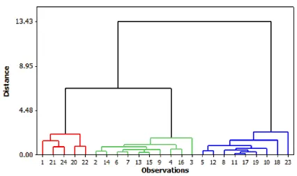
The results of a cluster analysis can be effectively summarized visually with the aid of a

dendogram. A dendogram is type of tree diagram with U-shaped links, which helps to

visualize the clusters produced by the unsupervised classification method described above.

The dendogram is constructed by plotting the distance versus the observation number, as

shown in Figure 3.3.

Figure 3.3: Sample Dendogram to Visualize Clusters

Figure 3.3, shows three distinct groups identified through cluster analysis since the

(36)

20

other. The distance between two individual groups, Ci and Cj can be determined using the

combinatorial expression presented in Equation 15 [14].

𝐷(𝐶𝑖, 𝐶𝑗) =

(𝑛_𝑗+ 𝑛_𝑘)𝑑_𝑘𝑗+ (𝑛_𝑗 + 𝑛_𝑙)𝑑_𝑙𝑗− 𝑛_𝑗𝑑_𝑘𝑙 𝑛𝑖 + 𝑛𝑗

(15)

where, 𝑑 is the Euclidean distance between the two vectors, ni, nj, nk, nl are the number of

observations in Ci, Cj, Ck, Cl. The new cluster Cj is considered to be formed by merging

two clusters Ck and Cl, respectively.

The distance between two respective clusters is sum of squared deviations from

points to cluster centroids [15]. It should be noted that the relative ranking of the distance

in the dendogram is more important in the formation of clusters rather than the magnitude

itself.

3.3 Factor Analysis

In addition to performing a cluster analysis to determine natural groups or clusters

in a data set, it is often beneficial to identify the underlying characteristics of the collected

data. This can be achieved through factor analysis by defining a small number of factors,

n, that can explain most of the variation observed in the data set. The main objective of

factor analysis is to provide logical interpretation of a multivariate data set by reducing

complexity through identification of factors, which can essentially explain most of the

model behaviour. Thus, a data set with x variables can be explained with the help of n

variables instead; where, n will always be smaller than x.

3.3.1 Factor Model

Assume a data set of variables y1, y2,…yx. Also, assume that all the variables in the

data set are linearly related to a small number of common factors (f1, f2,…,fn). These factors

are considered to be inferred from the relationship inherent to the data set, instead of being

collected directly from the data. Thus, each variable in the data set can be expressed as a

(37)

21

𝑦₁ = 𝛽 ₁₀+ 𝛽 ₁₁𝑓₁+ 𝛽 ₁₂𝑓₂+ ⋯ + 𝛽 _1𝑛𝑓_𝑛 + 𝑒₁ 𝑦₂ = 𝛽 ₂₀+ 𝛽 ₂₁𝑓₁+ 𝛽 ₂₂𝑓₂+ ⋯ + 𝛽 _2𝑛𝑓_𝑛+ 𝑒₂

𝑦_𝑥 = 𝛽 _𝑥0+ 𝛽 _𝑥1𝑓₁+ 𝛽 _𝑥2𝑓₂+ ⋯ + 𝛽 _𝑥𝑛𝑓_𝑛+ 𝑒_𝑥 (16)

In equation 16, e1, e2,…ex are considered as the errors between the actual values and the

predicted values of a given variable, by the factor model. Moreover, the terms β10, β21,…βfn

are the coefficients for the respective factors and are referred to as the factor loadings.

Hence, the abovementioned model is analogous to a regression model where each variable

can be modelled using n factors, which can explain the variation in the data set. At this

point, it should be realized that n << x.

Before a detailed discussion is presented on how to interpret the factor model, the following assumptions are necessary to uniquely estimate the parameters for the model

[13]:

1. The mean and variance of random errors, ei, are zero: 𝑒̅ = 0, and σe2 = 0, where i =

1, 2,…x.

2. The mean and variance of common factors, fi, is zero and one respectively: 𝑓̅ = 0, and σf2 = 1, where i = 1, 2,…n.

3. There is no correlation within common factors, errors, and between common factors

and errors: cov(fi, fj) =0, cov(ei, ej) = 0, and : cov(ei, fj) = 0.

Based on the assumptions presented for the model, the variance of any given variable

xi can be calculated using Equation 17.

𝜎𝑥𝑖

2 _{= 𝛾} 𝑖12𝜎𝑓1

2 _{+ 𝛾}

𝑖22𝜎𝑓2

2 _{+ … + 𝛾} 𝑖𝑛2 𝜎𝑓𝑛

2 _{+ (1}2_)𝜎 𝑒𝑖

2

𝜎𝑥𝑖

2 _{= 𝛾}

𝑖12 + 𝛾𝑖22 + … + 𝛾𝑖𝑛2 + 𝜎𝑖2

(17)

where, the terms 𝛾_𝑖12 + 𝛾_𝑖22 + … + 𝛾_𝑖𝑛2 are referred to as the communality, and 𝜎_𝑖2 is

referred to as the specific variance, of any give variable i. Communality represents the

(38)

22

Communality serves as a good assessment tool to determine how well the

developed factor model behaves with respect to a set of variables. Moreover, the covariance

between any two variables (xi, xj) can be determined using Equation 18.

𝑐𝑜𝑣(𝑥_𝑖, 𝑥_𝑗) = 𝛾_𝑖1𝛾_𝑗1+ 𝛾_𝑖2𝛾_𝑗2+ ⋯ + 𝛾_𝑖𝑛𝛾_𝑗𝑛 (18)

Once the variance and covariance are computed for all the variables using Equations 17

and 18, the results can be organized in a variance-covariance matrix, C, as explained in

Section 3.1.1. Matrix C will have a dimension of x x x, since there are x variables in the

data set.

The variance for each variable is organized along the major diagonal of the matrix,

while the covariance between the individual variables is arranged in the remainder

elements of the symmetric matrix, C. A matrix computed using original variables from the

data set leads to the formation of theoretical variance-covariance matrix. On the other hand,

computation of a matrix using the predicted variables from the factor model leads to the

formation of an observed variance-covariance matrix. The difference between the

theoretical and the observed matrices is stored in a new matrix known as the residual

variance-covariance matrix (RD), as shown in Equation 19. The structure of matrix RD is

similar to that of matrix C.

𝑅𝑒𝑠𝑖𝑑𝑢𝑎𝑙 𝑀𝑎𝑡𝑟𝑥, 𝑅𝐷 = 𝐶𝑡ℎ𝑒𝑜𝑟𝑒𝑡𝑖𝑐𝑎𝑙− 𝐶𝑝𝑟𝑒𝑑𝑖𝑐𝑡𝑒𝑑 (19)

The residual matrix helps to assess the fit of the factor model. The lower the values of the

residual matrix, the better the factor model performs in modelling the initial set of

variables, p, present the data set.

There are two methods widely used in factor analysis to determine the factor loading values for the model – principal component method and maximum likelihood

estimation method. The following section provides an overview of the principal component

method, since this method will be further used to analyse the multivariate driving data set.

Maximum likelihood estimation method requires the data set to be obtained from a

multivariate normal distribution data. Since not all variables necessarily follow a normal

distribution, principal component method was selected as the most suitable method for

(39)

23

3.3.2 Principal Component Method

The objective of the principal component method is to determine the factor loadings

in such a manner that the total communality of the model is as close as possible to the total

of the predicted variables. Principal component analysis will help to reduce the number of

variables in a data set for better interpretation, using linear combinations. Before the

principal component method is applied, it is very important for the data to be standardized.

The data standardization process and its implications are explained in further detail in

Chapter 5.

The first step, in determining the factor loadings using the principal component

method, is to construct the variance covariance matrix, C, of the data set using Equations

3 and 4. Since the variance covariance matrix is a square matrix, it can be re-represented

using eigenvalues and eigenvectors (Equation 8), as discussed in Section 3.1.2. Since the

idea is to reduce the dimension of the data set matrix, the eigenvector and the eigenvalues

are arranged in a descending order. Thus, the eigenvector with the highest eigenvalue forms

the first principal component and so on.

Once the principal components are identified, the factor loading can be determined

using the spectral decomposition (SD) theorem, as shown in Equation 20.

𝑆𝐷 = ∑ 𝜆_𝑖𝑣_𝑖𝑣_𝑖𝑇

𝑥

𝑖−1

=̃ ∑ 𝜆_𝑖𝑣_𝑖𝑣_𝑖𝑇

𝑛

𝑖−1

= 𝐿𝐿𝑇 ₍₂₀₎

where, v is the eigenvector corresponding to the eigenvalue λi, viT is the transpose of v, and

L is the factor loading matrix. Thus, the estimator of factor loadings [13] can be expressed

using Equation 21 as follows:

𝑙𝑖𝑗 = 𝑣𝑖𝑗√𝜆𝑖 (21)

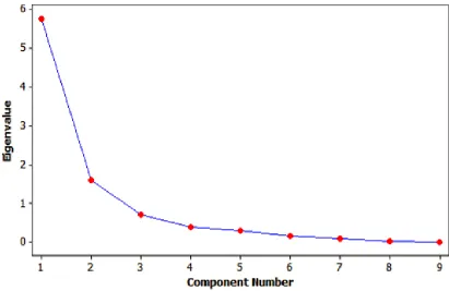
Finally, to determine the number of factors required for the analysis, a scree plot

can be generated by plotting the eigenvalues vs. the number of principal components, as

shown in Figure 3.4. The number of factors is determined at the point beyond which the

eigenvalues are comparably small and do not change significantly with respect to each

other. For instance, by observing Figure 3.4, it can be seen that beyond the third component,

(40)

24

components can be selected for use in the factor model. The interconnecting lines for scree

plots serve as a visual aid for determining the trend, the eigenvalues cannot assume any

values along the interconnecting lines (blue lines). The set of eigenvalues calculated for

each data set is discrete in nature.

(41)

25

CHAPTER 4 ARTIFICIAL NEURAL NETWORKS

4.1 Background

Artificial neural networks (ANN), as the name suggests, are inspired by biological

neurons and the information processing capabilities of the human brain. ANNs can be

described as massive interconnected processing elements (neurons) that can obtain and

store knowledge from an external environment or data set. From a mathematical

standpoint, neural networks can be considered as “black boxes”, and serve as an essential

analysis and modelling tool for multivariate data sets. ANNs are capable of performing a

variety of tasks including prediction (function approximation), pattern recognition, and

forecasting [16]. They are versatile tools used across multiple disciplines and areas of

research ranging from engineering systems and stock market predictions to speech pattern

recognition.

Traditional methods for determining the relationship between input and output

parameters require a set number of rules, equations, or assumptions for describing the

system. One of the biggest advantages of ANNs are that no prior assumptions or rules are

required to determine the underlying relationships between the input and the output

parameters. This thesis will focus on developing a classification ANN model for

categorizing driving performance using a known set of inputs and outputs. This technique

is known as supervised learning, where the network attempts to approximate the

relationship between the inputs and the different classes of driver performance using a

known set of targets or classes. The aim of this chapter is to provide introduction to the

concepts associated with the design and construction of classification neural networks. The

chapter concludes with some general design guidelines and evaluation methods to ensure

the quality, in terms of network accuracy and generalization capabilities, of any desired

network of choice.

4.2 Multi-Layer Perceptrons

As mentioned earlier, ANNs are built by interconnecting processing units called

(42)

26

weights that help the ANN to learn and map inputs to outputs. The weights are an integral

part of a network and help to describe the effect of each single unit on the network output.

For the purpose of this research, a specific type of neural network known as multi-layer

perceptrons (MLP) will be discussed. MLPs are one of the most widely used types of neural

networks [17], consisting of a set of input units and a set of output units connected together

through one or more processing hidden units. The hidden units will be primarily used as

non-linear classifiers to categorize driver performance. Such networks are arranged in

layers and will be represented henceforth as a series of three numbers in the following

format: Input layer – Hidden layer(s) – Output layer.

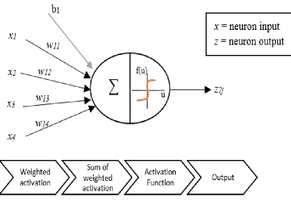
The number of inputs, hidden layer(s), and outputs will be expressed in numeric

format to provide an overview of the network architecture. For example, a basic

feedforward MLP network with a 4-2-1 architecture is presented in Figure 4.1. The term

feedforward indicates that information flows only in one direction in the network (i.e. from

inputs to outputs). No feedback loops are present in such networks.

A Method for Classifying Driver Performance

Scholarship at UWindsor

Scholarship at UWindsor

A Method for Classifying Driver Performance

A Method for Classifying Driver Performance

A Method for Classifying Driver Performance

A Method for Classifying Driver Performance

DECLARATION OF ORIGINALITY

ABSTRACT

DEDICATION

ACKNOWLEDGEMENTS

TABLE OF CONTENTS

LIST OF FIGURES

LIST OF APPENDICES

LIST OF ABBREVIATIONS/NOMENCLATURE

LIST OF SYMBOLS

CHAPTER 1

INTRODUCTION

CHAPTER 2

LITERATURE REVIEW

• Vehicle state

• Road geometry

and condition

• Driver workload

Inputs

• Vehicle control

• Risk perception

• Cognitive

processes

Information

Processing

• Safety

• Performance

evaluation

• Efficiency

CHAPTER 3

STATISTICAL METHODS

CHAPTER 4

ARTIFICIAL NEURAL NETWORKS

_{• Safety}