DOA and Polarization Estimation Algorithm Based on the Virtual
Multiple Baseline Theory
Guibao Wang1, *, Mingxing Fu1, Feng Zhao1, and Xiang Liu1, 2, 3
Abstract—An algorithm of solving phase ambiguity of multi-baseline direction finding system based on sparse uniform circular array is proposed in this paper. This sparse uniform circular array whose inter-element spacing is larger than half-wavelength distance suffers from cyclic phase ambiguities, which may cause estimation errors. In order to solve the above phase ambiguities, the corresponding virtual short baselines are acquired by transforming the array element phases that meet with the contraction relationship. The obtained short baselines are used to solve the phase ambiguities according to the virtual baseline and stagger baseline theory. Highly accurate estimates of direction of arrival are herein acquired. Furthermore, the direction of arrival and polarization parameter estimates are automatically matched with no additional processing. The array arrangement problem in high frequency scenario is solved. The estimation accuracy of angle of arrival is improved by means of the phase ambiguity resolution. Simulation results verify the effectiveness of this algorithm.
1. INTRODUCTION
Electromagnetic vector sensor array can obtain multi-dimensional information of electromagnetic signal, and it herein has the ability of spatial and polarization domain signal processing. The direction of arrival (abbreviated DOA) and polarization parameter estimations of multiple narrowband signals using electromagnetic vector sensor array techniques have a crucial role to play in many applications involving communication, radio astronomy, radar, sonar, seismic sensing, etc., and many valuable research results have been obtained [1–29]. Electromagnetic vector sensor can be divided into two categories: complete electromagnetic vector sensor (namely six-component electromagnetic vector sensor) and incomplete electromagnetic vector sensor (namely the antenna number of electromagnetic vector sensor is less than six). Particularly, the collocated loop and dipole pair has good performance because its antenna elements are not sensitive to the signal direction of arrival, which can decouple the polarization from direction of arrival [1–6].
A subspace algorithm to estimate direction of arrival and polarization by exploiting complete electromagnetic vector sensor was first proposed in [7–9]. Li and Compton [10] first applied estimations of signal parameters via rotational invariance techniques (abbreviated ESPRIT) to a vector-sensor array, and “vector-cross-product” DOA estimator was first applied to ESPRIT in [11, 12]. The uni-vector-sensor multiple signal classification (abbreviated MUSIC) algorithms were proposed in [13, 14]. Ref. [15] proposed an efficient two-dimensional direction finding method for improving estimation accuracy via aperture extension using the propagator method. The spread six-component electromagnetic vector-sensor direction-finding algorithms were proposed in [16, 17], which extended the spatial aperture at lower hardware cost. Ref. [18] proposed a novel disambiguation method using a MUSIC-like procedure to
Received 17 April 2016, Accepted 7 June 2016, Scheduled 21 June 2016 * Corresponding author: Guibao Wang ([email protected]).
identify the true direction cosine estimate from a set of cyclically related ambiguous candidate estimates. A novel closed-form ESPRIT-based algorithm using arbitrarily spaced electromagnetic vector-sensors was proposed in [19].
To ensure unambiguous angle estimations, it is required that the array inter-sensor spacing is less than half wavelength. However, the extended array aperture can offer enhanced array resolution but will cause the phase ambiguity of angle estimates. Therefore, resolving the phase ambiguity of array aperture extension is important [20–22], and the contribution of some work lies in that direction. Wang and co-authors proposed a DOA and polarization joint estimation method based on uniform concentric circular array [20], in which the phase differences between two array elements on inner circle were used to give rough but unambiguous estimates of DOA and as coarse references to disambiguate the cyclic phase ambiguities in phase differences between two array elements on outer ring circle. In [21], a two-dimensional DOA and polarization estimation algorithm for coherent sources using a linear vector-sensor array is presented. Yuan put forward the direction finding and polarization estimation method by using the spatially spread dipole/loop quads/quints in literature [22]. A 2-D direction finding algorithm with a sparse uniform array was introduced in [23], and the disambiguation of the resulting cyclic ambiguities was accomplished by the use of arrival angle information.
In this paper, we present a new phase ambiguity resolution approach based on the virtual multiple baseline theory [24–27]. The estimated phase differences are implemented by virtual array transformation when the phase differences of array elements satisfy certain conditions, and the ambiguous phase differences are herein resolved. The unambiguous but coarse phase differences are used to disambiguate the true phase differences of original array.
2. SIGNAL AND ARRAY MODELS
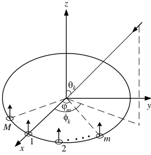
The receiving uniform circular array is composed ofM identical collocated loop and dipole pair, whose antenna elements are distributed over a circle with radius R. Supposing that the center of circle is located at the origin, the reference element of the array is a collocated loop and dipole, which is placed at origin, and the whole array elements are placed in the x-y plane, as shown in Fig. 1.
The collocated loop and dipole pairs’ steering vector of the kth (1 ≤ k ≤ K) unit-power electromagnetic source signal is 2×1 vector as follows:
ekz
hkz
=
−sinθksinγkejηk
sinθkcosγk
(1)
where θk ∈[0, π/2] is the signal’s elevation measured from the positivez-axis; γk ∈[0, π/2] symbolizes
the auxiliary polarization angle; ηk ∈[−π, π] represents the polarization phase difference. hkz and ekz
denote thez-axis magnetic and electric field received by loop and dipole at the origin of the coordinates.
K(K < M) narrowband completely polarized electromagnetic plane wave source signals from
far-field impinge upon an array, and the output of the uniform circular array at time t can be written
x
z
y
M
m
1 2
k
θ
φ ϕm
k
compactly as
X(t) =
B1
B2
S(t) +N(t) =BS(t) +N(t) (2)
whereX(t) is the received signal,Bthe (2M+ 2)×K array manifold matrix for theK incident signals, S(t) the incident signal andN(t) the noise. B1 and B2 are respective the sub-array steering vectors of M+ 1 loops andM + 1 dipoles, which can be represented as
B1 = [sinθ1cosγ1q(θ1, φ1), . . . ,sinθKcosγKq(θK, φK)] (3)
B2 =
−sinθ1sinγ1ejη1q(θ1, φ1), . . . ,−sinθKsinγKejηKq(θK, φK)
(4) where
q(θk, φk) =
1, ejϕk,1, . . . , ejϕk,m, ejϕk,M (5)
with the phase difference between the mth element and reference element of array ϕk,m defined in
Eq. (6).
ϕk,m=
2πR
λk
sinθkcos (φk−ϕm) (6)
where ϕm = 2π(m−1)/M, m= 1, . . . , M determines the angular location of antenna m on the circle,
and φk∈[−π, π] denotes the signal’s azimuth measured from the positivex-axis.
The true phase differences between theM elements and reference element of array can be obtained:
Φk= [ϕk,1, . . . , ϕk,m, . . . , ϕk,M] =
2πR
λk
W1Γk (7)
whereW1 is the matrix whose elements are involved in the array element angular position information,
so we call W1 as angular position information matrix. Γk is the vector whose elements are composed
of the direction cosine information. W1 and Γk have the following form:
W1 =
⎡ ⎢ ⎢ ⎢ ⎢ ⎢ ⎢ ⎣
0 1
sin 2π
M
cos 2π
M
..
. ...
sin
(M −1)2π
M
cos
(M −1)2π
M
⎤ ⎥ ⎥ ⎥ ⎥ ⎥ ⎥ ⎦
, Γk=
sinθksinφk
sinθkcosφk
(8)
From formulas (3) and (4), the following relationship can be obtained:
B2 =B1Φ (9)
where
Φ=
⎡ ⎢ ⎣
−tanγ1ejη1
. ..
−tanγKejηK
⎤ ⎥
⎦ (10)
3. DOA AND POLARIZATION ESTIMATION ALGORITHM
3.1. Polarization and Phase Difference Estimation Model
The covariance matrix Rx can be written as
Rx=EXXH=BRsBH+σ2I (11)
where Rs denotes the correlation matrix of incident signals and σ2 the white noise power. Let Es represent the (2M + 2) ×K matrix composing of the K eigenvectors corresponding to K largest eigenvalues of Rx. According to the subspace theory, there exists K×K nonsingular matrix T, and the signal subspace can be represented explicitly as [14]
Es=BT =
B1
B2
Since bothE1 and E2 are column full-rank, there is a unique nonsingular matrixΩsuch that
E1Ω = E2 ⇒Ω=
EH1 E1
−1
EH1 E2 (13)
ΩT−1 = T−1Φ (14)
It can be seen from Equation (14) that the estimation of Φ, namely ˆΦ, consists of K eigenvalues of matrix Ω, and the full-rank matrixT−1 is composed ofK eigenvectors of matrix Ω.
From matrix ˆΦ, the auxiliary polarization angle and polarization phase difference are obtained: ˆ
γk= tan−1Φˆk,k
ˆ
ηk= arg
−Φˆ
k,k
(15) The estimates ofB,B1 and B2 can be obtained by
ˆ
B1 =E1Tˆ−1 Bˆ2 =E2Tˆ−1 Bˆ =EsTˆ−1 (16)
The estimate of spatial steering vector ˆq(θk, φk) is obtained from the normalized Bˆ1:
ˆ
q(θk, φk) =
ˆ
B1(2 : M+ 1, k)
ˆ B1(1, k)
(17)
From formula (17), the estimated phase difference between the M elements and reference element of array can be obtained:
ˆ
Φk= arg [ˆq(θk, φk)] = [ ˆϕk,1, . . . ,ϕˆk,m, . . . ,ϕˆk,M] (18)
where ˆϕk,m is the estimated value of phase difference ϕk,m.
The sparse uniform circular array whose radius is larger than half maximum wavelength will suffer from phase ambiguities, that is to say, the estimated phase differences matrix ˆΦk and true phase differences matrix Φk meet the following relationship:
Φk= ˆΦk+ 2πpk (19)
where pk = [pk1, pk2, . . . , pkM] is the phase ambiguity vector. In order to obtain the exact direction of
arrival information, vector pk should be acquired.
3.2. Virtual Transformation and Phase Ambiguity Resolution
The virtual element of the array can be obtained by executing virtual transformations on two true array-elements. The phase difference between the kth virtual element and reference element of array can be expressed as follows:
ˆ
ϕk,n+ ˆϕk,m =
2πR
λk
sinθk[cos (φk−ϕn) + cos (φk−ϕm)]
= 2π
2RcosMπ (m−n)
λk
sinθkcos
φk− m
+n
2 −1
·2π
M
(20)
From Equations (6) and (20), the radius of the virtual circular array becomes R(1) =
2Rcos [π(m−n)/M] after one time virtual array transformation. The necessary condition for the operation of virtual array transformation is thatR(1) is less than R.
According to the relationship of R(1) andR, it can be obtained:
0<cos [π(m−n)/M]< 1
2 (21)
According to formula (21), the relationship of m andn can be obtained:
M/3< m−n < M/2 or M/3< n−m < M/2 (22)
3.2.1. The Case of Same Angular Position Information Matrix
When i = (m+n)/2 is integer, after one virtual array transformation, the phase difference matrix between the virtual M-element and reference element of array can be expressed as:
ˆ Φ(1)k =
ˆ
ϕ(1)k,1,ϕˆ
(1)
k,2, . . . , ϕˆ
(1)
k,M
(23)
where ˆϕ(1)k,i is the phase difference between theith (i= 1, . . . , M) virtual element and reference element of array, with
ˆ
ϕ(1)k,i = ˆϕk,n+ ˆϕk,m=
2πR(1)
λk
sinθkcos
φk−(i−1)·
2π M
(24)
From formula (24), there exists the following relationship: ˆ
Φ(1)k =T(1)k Φˆk (25)
whereT(1)k is the first time virtual array transformation matrix whose elements come from Equation (24). Since there exist phase ambiguities in ˆΦ(1)k , the virtual array transformation needs to be done, provided that the virtual circular radius is larger than incident signal half wavelength. Suppose that the virtual circular radiusR(L) is less than incident signal half wavelength after implementing Ltimes virtual array transformations, that is to say, R(L) < λk/2. According to formulas (6) and (20), the
following expression is obtained:
R(L)=R
2 cosπ(m−n)
M
L
(26)
Suppose that the phase difference matrix and virtual transformation matrix after Ltimes virtual transformations are labeled as ˆΦ(kL) andT(kL), then the following relationship can be obtained:
ˆ
Φk(L)=Tk(L)Φˆ(kL−1)=
T(1)k
L
ˆ
Φk (27)
with ˆΦ(kL) =
ˆ
ϕ(k,L1),ϕˆ
(L)
k,2, . . . ,ϕˆ
(L)
k,M
T
.
The matrices ˆΦ(kL) and R(L) also have the following form:
ˆ
Φ(kL)= 2πR
(L)
λk
W1Γˆk (28)
where ˆΓk=
sin ˆθksin ˆφk,sin ˆθkcos ˆφk
T
is the coarse and unambiguous estimation of direction cosine, and W1 is defined in Equation (8). SinceR(L) < λk/2, there does not exist phase ambiguity in ˆΦ
(L)
k ,
that is to say, the elements ˆϕ(k,iL) in ˆΦk(L) are in the range of −π to π, with 1≤i≤M. Based on the foregoing analysis, the following relationship can be obtained:
ˆ
Φk(L) =Tk(L)Φˆ(kL−1) =
T(1)k
L
ˆ
Φk= 2πR
(L)
λk
W1Γˆk (29)
The angular position information matrices of virtual and true circular arrays are the same, but the radii of the two arrays are different.
3.2.2. The Case of Different Angular Position Information Matrix
When i = (m+n)/2 is non-integer, let d = (m+n+ 1)/2, and d is the sequence number of the virtual array. After one time virtual array transformation, the phase difference matrix between the virtualM-element and reference element of array can be represented as:
ˆ Φ(1)k =
ˆ
ϕ(1)k,1,ϕˆ
(1)
k,2, . . . , ϕˆ
(1)
k,M
where ˆϕ(1)k,dis the phase difference between thedth (d= 1, . . . , M) virtual element and reference element
of array, with
ˆ
ϕ(1)k,d = ˆϕk,n+ ˆϕk,m=
2πR(1)
λk
sinθkcos
φk− d−
1 2
·2π
M
(31)
From formula (31), there exists the following relationship: ˆ
Φ(1)k =Tk1Φˆk (32)
where Tk1 is the first time virtual array transformation matrix whose elements are derived from
Equation (31), and ˆΦ(1)k is the phase difference matrix after the first time virtual array transformation. The relation of ˆΦ(1)k and R(1) can also be represented in matrix notation as follows:
ˆ
Φ(1)k = 2πR
(1)
λk
W2Γˆk (33)
whereW2 is the matrix whose elements denote the angular position information, i.e.,
W2 =
⎡ ⎢ ⎢ ⎢ ⎢ ⎢ ⎢ ⎢ ⎣
sin
π
M
cos
π
M
sin 3π
M
cos 3π
M
..
. ...
sin
(2M−1) π
M
cos
(2M−1) π
M
⎤ ⎥ ⎥ ⎥ ⎥ ⎥ ⎥ ⎥ ⎦
(34)
From formulas (8) and (34), we can see that the matrixW1 is different from W2.
After two times of virtual array transformations, the phase differences can be expressed as follows:
ˆ
ϕ(2)k,d = ˆϕ(1)k,n+ ˆϕ(1)k,m =
2πR(2)
λk
sinθkcos
φk−
d−1·2π
M
(35)
where m and n are the sequence numbers after one virtual transformation. Since i = (m+n)/2 is non-integer, d = (m+n−1)/2 is integer. Furthermore, the phase differences ˆϕ(2)k,d in Eq. (35) have
the same form as ˆϕ(1)k,i in Eq. (24).
Equation (35) can be indicated with the following matrix form:
ˆ
Φ(2)k = 2πR
(2)
λk
W1Γk (36)
Formula (35) can also be represented by the following matrix form ˆ
Φ(2)k =Tk2Φˆ (1)
k =Tk2Tk1Φˆk (37)
where Tk2 and ˆΦ (2)
k are the virtual array transformation matrix and phase difference matrix after two
times of virtual array transformation, which are determined by formula (35). Based on the above-mentioned analysis, it can be shown that the virtual angular position information matrix is the same as the true angular position information matrix after two times of virtual transformations. Meanwhile, the radii of the virtual circular array and initial circular arrays are different.
The true phase difference matrix can be obtained if R(1) or R(2) is less than incident signal half wavelength. Otherwise, ˆΦ(1)k or ˆΦ(2)k has phase ambiguities, and the virtual transformation herein needs to be continued until the virtual circular radius is less than incident signal half wavelength. Supposing that R(L) defined in formula (26) is less than half wavelength of the incident signal after conducting
L times virtual transformations, the corresponding phase difference matrix is labeled as ˆΦ(kL), whereL
1) The number of virtual array transformation timesL is odd, and the relation between ˆΦ(kL) and ˆΦk are summarized as follows:
ˆ
Φ(kL) = 2πR
(L)
k
λk
W2Γˆk =Tk1(Tk2Tk1) L−1
2 Φˆk (38)
where L is the minimal positive even number that meets R(L) < λk/2, andR(L) has the form in
Equation (26). ˆΦk is the original phase difference matrix.
2) The number of virtual array transformation times L is even, and the relation between ˆΦ(kL) and ˆ
Φk are summarized as follows:
ˆ
Φ(kL) = 2πR
(L)
k
λk
W1Γˆk = (Tk2Tk1) L
2 Φˆk (39)
3.3. Phase Ambiguity Resolution in Direction Finding
According to Equations (29), (38) and (39), we get the coarse and unambiguous estimate ˆΓk: ˆ
Γk=W#Φˆ(kL) =W#T(kL)Φˆ (40) whereW#=WHW−1WH is a pseudo-inverse matrix of W, with
⎧ ⎪ ⎪ ⎪ ⎪ ⎪ ⎪ ⎪ ⎪ ⎨ ⎪ ⎪ ⎪ ⎪ ⎪ ⎪ ⎪ ⎪ ⎩
W= 2πR
(L)
k
λk
W1, T(kL)= (Tk)L when m
+n
2 and L are intergers
W= 2πR
(L)
k
λk
W2, T (L)
k =Tk1(Tk2Tk1) L−1
2 when m+n
2 is non-interger, Lis odd number
W= 2πR
(L)
k
λk
W1, T(kL)= (Tk2Tk1) L
2 when m+n
2 is non-interger, Lis even number
.
By substitution of Eq. (40) into Eq. (41), the coarse but unambiguous estimations of the true phase difference matrix ¯Φare obtained as follows:
¯
Φk = 2πR
λk
W1Γˆk (41)
From formulas (19) and (41), a method is developed for solving the phase cycle number ambiguity vector pk, opt, and this problem is formulated as the optimization procedure:
pk, opt= arg min
pk Φ¯ k− ˆ
Φk+ 2πpk (42)
From Eq. (42), the estimates of true phase difference matrix ˜Φcan be obtained as: ˜
Φk= ˆΦk+ 2πpk, opt (43)
Here ˜Φis the high-precision estimation.
According to Equations (7) and (43), it is shown that ˜
Φk=EkΓ˜k (44)
where
Ek= 2πR
λk
W1 Γ˜k=
˜
Γk1
˜ Γk2
=
sin ˜θksin ˜φk
sin ˜θkcos ˜φk
(45)
The accurate direction cosine estimates are obtained by employing the least square norm: ˜
Γk=
˜
Γk1
˜ Γk2
=
sin ˜θksin ˜φk
sin ˜θkcos ˜φk
whereE#k =EHkEk−1EHk is a pseudo-inverse matrix of Ek.
According to formula (46), the accurate estimates of direction of arrival are obtained:
⎧ ⎪ ⎪ ⎪ ⎪ ⎪ ⎪ ⎪ ⎪ ⎨ ⎪ ⎪ ⎪ ⎪ ⎪ ⎪ ⎪ ⎪ ⎩
˜
θk= arcsin
˜
Γ2k1+ ˜Γ2k2
⎧ ⎪ ⎪ ⎪ ⎪ ⎨ ⎪ ⎪ ⎪ ⎪ ⎩
˜
φk= arctan
˜ Γk1
˜ Γk2
, Γ˜k2≥0
˜
φk=π+ arctan
˜ Γk1
˜ Γk2
, Γ˜k2<0
(47)
Our proposed virtual transformation method for estimating the direction of arrival and polarization parameters can herein be summarized as follows.
1) Measure the phase differences ˆΦk between the array element and the origin of coordinate, and ˆΦk is ambiguous.
2) The matrix ˆΦ(kL) whose phase difference is unambiguous, and the coarse estimates of direction cosine ˆΓk are obtained according to the virtual transformation Equation (40).
3) The number of phase cycle ambiguities of the true phase difference matrix is acquired according to formula (42), thus the true phase difference matrix ˜Φk is achieved, and the DOA estimates are herein obtained.
4. SIMULATION RESULTS
In this section, the direction of arrival and polarization parameter estimation experiments are carried out to verify the effectiveness of the proposed method. Incident signal source with parameters (θ1, φ1, γ1, η1) = (28◦,45◦,65◦,78◦) and (θ2, φ2, γ2, η2) = (72◦,85◦,35◦,120◦) impinge upon a sparse
7-element uniform circular array with a radius ofR = 3.5λ, as shown in Fig. 1. 200 independent Monte Carlo trials and 512 temporal snapshots are used in these simulations. The simulation results are shown in Figs. 2–8.
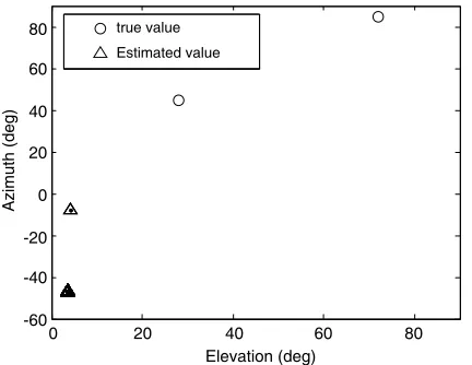
In the first experiment, we consider the scatter diagrams of elevation and azimuth. The signal-to-noise ratio (abbreviated SNR) is set to 15 dB, and the sets of values of the DOA variables have been represented in Figs. 2 and 3.
The true values of direction of arrival are (θ1, φ1) = (28◦,45◦) and (θ2, φ2) = (72◦,85◦). From
Fig. 3, we can see that the perturbation of the estimated values using virtual array is small, and the estimated values of direction of arrival, namely ˆθ1 and ˆφ1, are respectively the numerical ranges
0 20 40 60 80
Elevation (deg) 0
20 40 60 80
-20 -40 -60
Azimuth (deg)
true value
Estimated value
Figure 2. Scatter diagram using original array.
30 40 50 60 70
Elevation (deg) 60
70 80 90
50
40
Azimuth (deg)
30 40 50 SNR (dB)
0 10 20
RMSE of Elevation (deg)
10
10
10
10
10 4
2
0
-2
-4
Estimation of original array
Estimation of virtual array
Figure 4. RMSE of elevation versus SNR.
30 40 50
SNR (dB)
0 10 20
RMSE of Azimuth (deg)
10
10
10
10
10 4
2
0
-2
-4
Estimation of original array
Estimation of virtual array
Figure 5. RMSE of azimuth versus SNR.
ˆ
θ1∈(27.9◦,28.1◦) and ˆφ1 ∈(44.85◦,45.15◦). Similarly, the estimated values of ˆθ2 and ˆφ2are respectively
the numerical ranges θ2 ∈ (71.8◦,72.2◦) and φ2 ∈ (84.8◦,85.2◦). On the contrary, using the original
array the estimated points of azimuth are wrongly distributed in the ranges of φ1 ∈ (−7.75◦,−7.65◦)
and φ2∈(−46.7◦,−47.3◦), and the estimated points of elevation are wrongly distributed in the ranges
of θ1 ∈(4.16◦,4.18◦) and θ2∈(3.48◦,3.52◦), as shown in Fig. 2.
In the second experiment, we consider the performance of the estimations of DOA and polarization. Without loss of generality, we discuss only the signal one. The root mean square error (abbreviated RMSE) of the DOA and polarization variables are represented in Figs. 4–7, and the SNR ranges in Figs. 4-7 are from 0 dB to 50 dB.
Figure 4 shows that the RMSE of elevation using original array is 27.55◦. The RMSE of elevation using the virtual array is 0.053◦ at SNR = 0. Moreover, the RMSE of elevation decreases evidently as the SNR increases. Similarly, the RMSEs of azimuth using the original and virtual array are indicated in Fig. 5, and the RMSE of azimuth using the original array is 69◦. In the SNR range (namely, at or above 0 dB), the RMSE of azimuth is degraded significantly using the virtual array, and the RMSE of azimuth is 0.09◦ at SNR = 0. The reason that the estimation using original array has larger deviation is as follows: the existence of phase ambiguity makes the estimates have larger deviation, which cannot be overcome even if improving the SNR. The virtual transform processing can effectively solve the problem of phase ambiguity. Hence the precise estimates of DOA can be obtained.
Figures 6–7 respectively plot the estimation RMSE of polarization phase difference and auxiliary polarization angle, respectively estimated using the virtual array and original array, at various SNR levels. The two estimated results are nearly the same because the sparse embattle of uniform circular array has little influence on polarization phase difference and auxiliary polarization angle.
In Figs. 4 and 5, the RMSE using the original array is plotted as the horizontal line, because the phase ambiguities exist, and then the estimates have larger deviations. For example, the average estimated value of elevation using the original array is 28◦ and the corresponding average estimated values of azimuth is 69◦. The disturbances of all the estimated values appear around the average estimated values. The disturbances grow smaller and smaller with the increase of SNR, which is too small relative to the average deviation to be shown in Figs. 4 and 5.
10 15 20 SNR (dB)
5 0
RMSE of Polarization Phase Difference (deg)
Estimation of original array Estimation of virtual array
-5 5
0 4
3
2
1
Figure 6. RMSE of polarization phase difference versus SNR.
10 15 20
SNR (dB) 5 0
RMSE of Auxiliary Polarization Angle (deg)
Estimation of original array Estimation of virtual array
-5 1.8
0 1.2
0.8
0.2 1.6 1.4
1
0.6 0.4
Figure 7. RMSE of auxiliary polarization angle versus SNR.
are similar to that of the elevation.
30 40 50
SNR (dB)
0 10 20
Standard Deviation of Elevation (deg)
10
10
10
10 -1
-2
-3
-4
Estimation of original array Estimation of virtual array
Figure 8. Standard deviation of elevation versus SNR.
5. CONCLUSION
ACKNOWLEDGMENT
This work was supported by the National Natural Science Foundation of China (61475094, 61201295) and also supported by the projects program of Shaanxi University of Technology Academician Workstation (fckt201504). The authors would like to thank the anonymous reviewers and the associated editor for their valuable comments and suggestions that improved the clarity of this manuscript. We also thank L. M. Wang very much for all the help she gave us when we wrote this manuscript.
REFERENCES
1. Yuan, X., K. T. Wong, Z. Xu, and K. Agrawal, “Various compositions to form a triad of collocated dipoles/loops, for direction finding and polarization estimation,” IEEE Sens. J., Vol. 12, No. 6, 1763–1771, 2012.
2. Wang, G., “A joint parameter estimation method with conical conformal CLD pair array,”Progress In Electromagnetics Research C, Vol. 57, 99–107, 2015.
3. Li, Y. and J. Q. Zhang, “An enumerative nonlinear programming approach to direction finding with a general spatially spread electromagnetic vector sensor array,” IEEE Trans. Signal Process., Vol. 93, 856–865, 2013.
4. Yuan, X., K. T. Wong, and K. Agrawal, “Polarization estimation with a dipole pair, a dipole-loop pair, or a dipole-loop-dipole-loop pair of various orientations,”IEEE Trans. Antenn. Propag., Vol. 60, No. 5, 2442–2452, 2012.
5. Luo, F. and X. Yuan, “Enhanced ‘vector-cross-product’ direction-finding using a constrained sparse triangular-array,” EURASIP J. Adv. Signal Process., Vol. 2012, No. 115, 1–11, 2012.
6. Wang, L. M., Z. H. Chen, and G. B. Wang, “Direction finding and positioning algorithm with COLD-ULA based on quaternion theory,” Journal of Communications, Vol. 9, No. 10, 778–784, 2014.
7. Nehorai, A. and E. Paldi, “Vector-sensor array processing for electromagnetic source localization,”
25th Asilomar Conf. Signals, Syst., Comput., 566–572, Pacific Grove, CA, 1991.
8. Nehorai, A. and E. Paldi, “Vector sensor array processing for electromagnetic source localization,”
IEEE Trans. Signal Process., Vol. 42, No. 2, 376–398, 1994.
9. Li, J., “Direction and polarization estimation using arrays with small loops and short dipoles,”
IEEE Trans. Antenn. Propag., Vol. 41, No. 3, 379–387, 1993.
10. Li, J. and R. T. Compton, “Two-dimensional angle and polarization estimation using the ESPRIT algorithm,”IEEE Trans. Antenn. Propag., Vol. 40, No. 5, 550–555, 1992.
11. Wong, K. T. and M. D. Zoltowski, “Polarization diversity and extended aperture spatial diversity to mitigate fading-channel effects with a sparse array of electric dipoles or magnetic loops,” IEEE Int. Veh. Technol. Conf., 1163–1167, 1997.
12. Wong, K. T. and M. D. Zoltowski, “High accuracy 2D angle estimation with extended aperture vector sensor arrays,”Proc. IEEE. Int. Conf. Acoust., Speech, Signal Processing, Vol. 5, 2789–2792, 1996.
13. Wang, L. M., L. Yang, G. B. Wang, and Z. H. Chen, “Uni-vector-sensor dimensionality reduction MUSIC algorithm for DOA and polarization estimation,” Math. Probl. Eng., Vol. 2014, 1–9, 2014. 14. Wong, K. T. and M. D. Zoltowski, “Uni-vector-sensor ESPRIT for multisource azimuth, elevation,
and polarization estimation,” IEEE Trans. Antenn. Propag., Vol. 45, No. 10, 1467–1474, 1997. 15. He, J. and Z. Liu, “Extended aperture 2-D direction finding with a two-parallel-shape-array using
propagator method,”IEEE Antenn. Wirel. Pr., Vol. 8, 323–327, 2009.
16. Wong, K. T. and X. Yuan, “Vector cross-product direction-finding’ with an electromagnetic vector-sensor of six orthogonally oriented but spatially non-collocating dipoles/loops,”IEEE Trans. Signal Process., Vol. 59, No. 1, 160–171, 2011.
18. Zoltowski, M. D. and K. T. Wong, “Closed-form eigenstructure-based direction finding using arbitrary but identical subarrays on a sparse uniform rectangular array grid,”IEEE Trans. Signal Process., Vol. 48, No. 8, 2205–2210, 2000.
19. Wong, K. T. and M. D. Zoltowski, “Closed-form direction-finding with arbitrarily spaced electromagnetic vector-sensors at unknown locations,”IEEE Trans. Antenn. Propag., Vol. 48, No. 5, 671–681, 2000.
20. Wang, L. M., G. B. Wang, and Z. H. Chen, “Joint DOA-polarization estimation based on uniform concentric circular array,” Journal of Electromagnetic Waves and Applications, Vol. 27, No. 13, 1702–1714, 2013.
21. Liu, J., Z. Liu, and Q. Liu, “Direction and polarization estimation for coherent sources using vector sensors,”Journal of Systems Engineering and Electronics, Vol. 24, No. 4, 600–605, 2013.
22. Yuan, X., “Spatially spread dipole/loop quads/quints: For direction finding and polarization estimation,” IEEE Antennas Wireless Propag. Lett., Vol. 12, 1081–1084, 2013.
23. Zoltowski, M. D. and K. T. Wong, “ESPRIT-based 2D direction finding with a sparse array of electromagnetic vector-sensors,” IEEE Trans. Signal Process., Vol. 48, No. 8, 2195–2204, 2000. 24. Gavish, M. and A. J. Weiss, “Array geometry for ambiguity resolution in direction finding,”IEEE
Trans. Antenn. Propag., Vol. 44, No. 6, 889–895, 1996.
25. Zhou, Y. Q. and F. K. Huang, “Solving ambiguity problem of digitized multi-baseline interferometer under noisy circumstance,” Journal of China Institute of Communications, Vol. 34, No. 8, 16–21, 2005.
26. Wang, L. M., J. P. Lin, G. B. Wang, and Z. H. Chen, “A direction finding technique using millimeter-wave interferometer,”J. Infrared Millim. W., Vol. 34, No. 2, 140–144, 2015.
27. Wu, Y. W., S. Rhodes, and E. H. Satorius, “Direction of arrival estimation via extended phase interferometry,”IEEE Trans. Aero. Elec. Sys., Vol. 31, No. 1, 375–381, 1995.
28. Wang, G. B., “Direction of arrival and polarization estimation with a polarized circular array,”
Journal of Beijing University of Posts and Telecommunications, Vol. 39, No. 2, 72–75, 2016. 29. Lomin´e, J., C. Morlaas, C. Imbert, and H. Aubert, “Dual-band vector sensor for direction of