www.ijiset.com
306
Application Of AHP Method For Optimal
Placement Of SSS
C Device Using TLBO
Sathupati keziaP
1
P
, Dr K PadmaP
2
P
1
P
Department of Electrical Engineering, Andhra University, Visakhapatnam, Andhra Pradesh, India
P
2
P
Department of Electrical Engineering, Andhra University, Visakhapatnam, Andhra Pradesh, India
ABSTRACT
The concept of FACTS (Flexible Alternating Current Transmission System) refers to a family of power electronics-based devices able to enhance AC system controllability and stability and to increase power transfer capability. FACTS devices, thanks to their speed and flexibility, are able to provide the transmission system with several advantages such as: transmission capacity enhancement, power flow control, transient stability improved, and power oscillation damping and voltage stability. This paper investigates modeling and analysis of Static Series Synchronous Compensator (SSSC) and performance of SSSC in power system. The ability of these FACTS devices for power flow control of normal/steady state condition is examined. The ability of FACTS device with AHP method using Teacher Learning Based Optimization (TLBO) method is also examined. This paper shows the Optimal Location of Static Series Synchronous Compensator (SSSC) in Transmission line using TLBO based AHP method. The objective is to minimize the fuel cost of generation, voltage deviation, transmission losses and to determine the optimal value of control variables such as generator real power, generator voltage magnitudes, tap setting of the transformer and number of compensation devices and also maintain a reasonable system performance in terms of limits on generator real power and reactive power outputs, bus voltages and power flow of transmission lines. The proposed method is examined and implemented on IEEE 30-bus power system network.
Keywords: -Analytical hierarchy process, static series synchronous compensator, Teacher learning based optimization.
1. Introduction
Modern power system networks are being operated under highly stressed conditions due to continuous increase
in power demand. This has imposed the threat of maintaining the required bus voltage and thus the systems have
been facing voltage instability problem. Voltage stability refers to the potency of the system to sustain the
sufficient voltage under normal operating condition, whereas the voltage instability refers to the lack of voltage
stability, which results in a continuous voltage decrease or increase. Using Flexible Alternating Current
Transmission System (FACTS) devices, the voltage stability and steady state and transient stabilities of a
stressed power system can be enhanced effectively. The power system network can be modified to alleviate
voltage instability or collapse by adding FACTS devices at the appropriate locations. FACTS devices can
control the active and reactive power as well as become adaptive to voltage-magnitude control simultaneously,
because of their flexibility and fast control characteristics. The devices are mainly used in power systems for
increasing the power transmission capability, enhancing static and dynamic stability, increasing the availability
and reducing the transmission loss. Also, the devices have the ability to control the parameter and variables of
the transmission line, such as line impedance, terminal voltages and voltage angle in a rapid and effective
307
2. Voltage stability index
Voltage stability refers to the ability of a power system to maintain steady voltages at all buses in the system
after being subjected to a disturbance from a given initial operating condition. It depends on the ability to
maintain/restore equilibrium between load demand and load supply from the power system. Voltage instability
occurs in the form of a progressive fall or rise of voltages of some buses.
∑
=−
=
g i j i ji jV
V
F
L
11
(1)Where the voltage stability index limit must lie between 0 to 1.
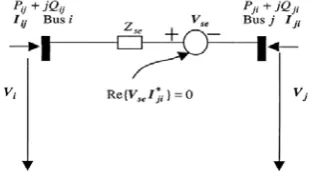
3. Modeling of Static Series Synchronous Compensator (SSSC)
A SSSC usually consists of a coupling transformer, an inverter and a capacitor. The SSSC is series connected
with a transmission line through the coupling transformer.
Figure 1: Equivalent Circuit of SSSC
The equivalent circuit of SSSC is as shown in the Figure 1. From the equivalent circuit the power flow
constraints of the SSSC can be given as
))
sin(
)
cos(
(
)
sin
cos
(
2 se i ij se i ij se i ij ij ij ij j i ii i ijb
g
V
V
b
g
V
V
g
V
P
θ
θ
θ
θ
θ
θ
−
+
−
−
+
−
=
(2)))
cos(
)
sin(
(
)
cos
sin
(
2 se i ij se i ij se i ij ij ij ij j i ii i ijb
g
V
V
b
g
V
V
b
V
Q
θ
θ
θ
θ
θ
θ
−
−
−
−
−
−
−
=
(3)))
sin(
)
cos(
(
)
sin
cos
(
2 se j ij se j ij se j ji ij ji ij j i ji j jib
g
V
V
b
g
V
V
g
V
P
θ
θ
θ
θ
θ
θ
−
+
−
+
+
−
=
(4)))
cos(
)
sin(
(
)
cos
sin
(
2 se j ij se j ij se j ji ij ji ij j i jj j jib
g
V
V
b
g
V
V
b
V
Q
θ
θ
θ
θ
θ
θ
−
−
−
+
−
−
−
=
(5) Where ij jj ij jj ij ii ij ii se ijij jb Z g g b b g g b b
g + =1/ , = , = , = , = Operating constraint of the SSSC (active
power exchange via the DC link) is as
www.ijiset.com
308
The active power flow constraint is
0
=
−
specifiedji ji
P
P
(7)0
=
−
specifiedji ji
Q
Q
(8)Where z is specified active power flow
The equivalent voltage injection
V
se∠
θ
se bound constraints are asmax min
se se se V V
V ≤ ≤ (9)
max min
se se se
θ
θ
θ
≤ ≤ (10)4. Teaching Learning Based Optimization Algorithm (TLBO)
Teaching Learning Based Optimization Algorithm is a new kind of population based global Rao et al in 2011.As
in other population population-based algorithms, in TLBO, The basic idea of TLBO is that the teacher is
considered as the most knowledgeable person in a class who shares his/her knowledge with the students to
improve the output (i.e., grades or marks) of the class. The quality of the learners is evaluated by the mean value
of the student’s grade in class. Furthermore, learners also learn from interaction between themselves, which also
helps in their results. The demonstration or working of TLBO Algorithm is divided into two parts:
1. “Teacher phase”.
2. “Learner phase”.
The first part consists of the “Teacher Phase” and the second part consists of the “Learner Phase”. The “Teacher
Phase” means learning from the teacher and the “Learner Phase” means learning through the interaction
between learners. TLBO searches for the global optimum mainly through two steps: teacher phase and learner
phase.
4.1 Teacher Phase
It is the first part of the algorithm where learners learn through the teacher. During this phase, a teacher tries to
increase the mean result of the class in the subject taught by him or her depending on his or her capability. The
difference between the existing mean result of each subject and the corresponding result of the teacher for each
subject is given by,
Difference_Mean𝑗,𝑘,𝑖=𝑟𝑖(𝑋𝑗,𝑘𝑏𝑒𝑠𝑡,𝑖− 𝑇𝐹𝑀𝑗,𝑖) (11)
Where,𝑋𝑗,𝑘𝑏𝑒𝑠𝑡,𝑖 i is the result of the best learner in subject j. TF is the teaching factor which decides the value of
mean to be changed, and 𝑟𝑖 is the random number in the range [0, 1]. Value of𝑇𝐹 can be either 1 or 2. The value
of 𝑇𝐹 is decided randomly with equal probability as,
TF = round [1+rand (0, 1) {2 -1}] (12)
TFis not a parameter of the TLBO algorithm the existing solution is updated in the teacher phase according to
the following expression.
Xj,k,iʼ = Xj,k,i+ Difference_Meanj,k,i (13)
Where;𝑋𝑗,𝑘,𝑖ʼ is the updated value of 𝑋𝑗,𝑘,𝑖 . 𝑋𝑗,𝑘,𝑖ʼ is accepted if it gives better function value. The learner phase
309
4.2 Learner Phase
A learner interacts randomly with other learners for enhancing his or her knowledge. The random inter- action
among learners improves his or her knowledge. In this stage a teacher choose a student randomly and tries to
enhance his information and knowledge by means of interaction.
Xj,P,iʼʼ = Xj,P,iʼ +ri�Xj,P,iʼ −�, If Xtotal−P,iʼ ˂Xtotal−Q,iʼ (14)
Xj,P,iʼʼ = Xj,P,iʼ +ri�Xj,Q,iʼ Xj,P,iʼ �, If Xtotal−Q,Iʼ ˂Xtotal−P,iʼ (15)
The equations (14) and (15) are for minimization problems. In the case of maximization problems, the eqs. (16)
And (17) are used.
Xj,P,iʼʼ = Xj,P,iʼ +ri�Xj,P,iʼ − Xj,Q,iʼ �, IfXtotal−Q,iʼ ˂Xtotal−P,iʼ (16)
Xj,P,iʼʼ = Xj,P,iʼ +ri�Xj,Q,iʼ − Xj,P,iʼ �, IfXtotal−P,Iʼ ˂Xtotal−Q,iʼ (17)
4.3 Pseudo Code for Teaching Learning Base Optimization Algorithm (TLBO)
STEP 1: Initialization
Step 1.1. : Generate a well-distributed set of N weighting vectors 𝑤𝑗= �𝑤1𝑗, … . . , 𝑤𝑚𝑗�, j=1,…, N and find
the neighborhood of each sub-problems: B (j) = { 𝑤𝑗,……,𝑤𝑗}.
Step 1.2.: Generate the initial population and evaluate its fitness.
Step 1.3. : Initialize the reference point𝑧∗.
STEP 2: For j= 1 to N do
Step 2.1. : Determine the class according to: C=� 𝐵(𝑗) 𝑖𝑓 𝑟𝑎𝑛𝑑 ˂𝛿
{1, … . , 𝑁} 𝑜𝑡ℎ𝑒𝑟𝑤𝑖𝑠𝑒
Where rand is a random number within [0,1] and 𝛿 the probability to select the neighborhood as the class.
Step 2.2. : Teacher phase
Step 2.3. : Update the reference point𝑧∗.
Step 2.4. : Update (𝑆𝑟) solutions. Where (𝑆𝑟) is the maximal number of solutions replaced by each new
solution obtained.
STEP 3: For j= 1 to N do
Step 3.1. : Determine the class according to: C=� 𝐵(𝑗) 𝑖𝑓 𝑟𝑎𝑛𝑑 ˂𝛿
{1, … . , 𝑁} 𝑜𝑡ℎ𝑒𝑟𝑤𝑖𝑠𝑒
Step 3.2. : Learner Phase
Step 3.3. : Update the reference point𝑧∗.
Step 3.4. : Update (𝑆𝑟) solutions.
www.ijiset.com
310
5. Mathematical Model of OPF Problem
Four types of objective functions of OPF problem are identified as below:
Objective Function I: Min
2 1
1
(
)
(
)
ng
i gi i gi i i
f
F pg
a P
b P
c
=
=
=
∑
+
+
Is total generation cost functionObjective Function II: Min
1
2 2 2
1
[
2
cos(
)]
N
L k i j i j i J
i
f
P
g V
V
VV
δ δ
=
=
=
∑
+
−
−
Is total real power loss.Objective Function III: Min 3 2
1
2
nb
j j g
f
Lj s
L
= +
=
=
∑
is the sum of squared voltage stability index.Objective Function IV: Min
2
4
1
(
1)
nb
i i
f
VD
V
=
=
=
∑
−
is the total voltage deviation.5.1 Constraints
The OPF problem has two categories of constraints.
5.1.1 Equality Constraints
These are the sets of nonlinear power flow equations that govern the power system, i.e.,
• load flow constraints:
0
)
cos(
1
=
+
−
−
−
∑
=
j i ij ij
j n
j i Di
Gi
P
V
V
Y
P
θ
δ
δ
(18)
0
)
sin(
1
=
+
−
+
−
∑
= j ij ij i j
n
j i Di
Gi
Q
V
V
Y
Q
θ
δ
δ
(19)
where
P
Gi andQ
Gi are the real and reactive power outputs injected at bus irespectively, the load demand atthe same bus is represented by
P
Di andQ
Di, and elements of the bus admittance matrix are represented byij
Y
and
θ
ij.5.1.2 Inequality Constraints
These are the set of constraints that represent the system operational and security limits like the bounds on the
following:
• Generators real and reactive power output
ng
i
P
P
P
Gi Gi Gi,
1
,
,
maxmin
=
≤
≤
(20)
Q
GiQ
GiQ
Gi,
i
1
,
,
ng
maxmin
=
≤
311
• Voltage magnitudes at each bus in the network
NL
i
V
V
V
i i i,
1
,
,
maxmin
=
≤
≤
(22)
Where NL is the number of load buses
• Transformer taps settings:
nt
i
T
T
T
i i i,
1
,
,
maxmin
=
≤
≤
(23)Where nt is the number of tap changing transformers
• Reactive power injections due to capacitor banks:
cs
i
Q
Q
Q
Cimin≤
Ci≤
Cimax,
=
1
,
,
(24)
Where cs is the number of shunt capacitor
• Transmission lines loading:
nl
i
S
S
i i,
1
,
,
max
=
≤
(25)
• Voltage stability index:
•
L
jL
j,
j
1
,
,
NL
max
=
≤
(26)
• FACTS device constraint:
min max
cR cR cR
V
≤
V
≤
V
SSSC voltage magnitude (27)
min max
cR cR cR
θ
≤
θ
≤
θ
SSSC voltage angle (28)
5.2 Overall Computational Procedure for Solving the Problem
The implementation steps of the proposed TLBO based algorithm can be written as follows:
Step 1: Input the system data for load flow analysis using economical dispatch approach.
Step 2: Select a FACTS device and its location in the system.
Step 3: Initial population (the number of learners) is generated using the design variables which are the amount
of rescheduling required by generators to manage congestion, (randomly within the limits).
Step 4: Using the generated (new) learners, the fitness function is evaluated (teacher phase).
Step 5: Mean of each design variable is computed and the best solution is identified as teacher among the
learners based on their fitness value.
Step 6: All other learners are modified with reference to the mean and the fitness function is evaluated using the
modified learners. Any two learners are randomly selected and their fitness values are compared. The student
with better fitness value is accepted while the other is rejected (learner phase).
Step 7: Run the newton Raphson load flow for updated values from teacher phase for the improvement of the
performance analysis.
Step 8: Repeat Step4, until all the learners participating in the test, confirms that any two learners do not repeat
the test.
Step 9: If maximum number of iteration is reached then the program is stopped otherwise it goes back to Step 3.
www.ijiset.com
312
6. Analytical Hierarchy process (AHP)
AHP is a decision-making tool, which helps in finding alternatives among alternative. It is a systematic method
for comparing a list of objectives and the alternative
Solutions satisfying respective objectives. Some mathematical steps involved in AHP method are as follows.
Step 1: selection and evaluation of attributes
Step 2: selection of alternatives
Step 3: Formation of decision matrix
Step 4: construction of pair wise comparison matrix
Step 5: Find the relative normalized weight.
Step6: Calculate matrices
A
3
and A4such thatA
3
=
A
1* 2
A
andA
4
=
A
3 / 2
A
, where A1is pair wisecomparison matrix,
2
(
1,
2,
3...
)
T jA
=
W W W
W
.Step7: Determine the maximum Eigen value
λ
max that is the average of matrixA
4.Step8: Calculate the consistency index ( max )
1
M
CI
M
λ −
=
−
. The smaller the value ofCI
, the smaller is thedeviation from the consistency
Step10: Calculate the consistency ratio
CR CI RI
=
/
. UsuallyCR
of 0.1 or less is considered as acceptableand it reflects an informed judgment attributable to the knowledge of the analyst regarding the problem under
study.
Step11: The overall performance score of the alternatives is obtained by multiplying the relative normalized
weight (
W
j) of each attribute with its corresponding normalized weight value for each alternative and summingover the attributes for each alternative.
7. RESULTS AND DISCUSSION
The proposed TLBO algorithm is applied for solving optimal power flow problem on standard IEEE-30bus
system without and with SSSC device installation.
7.1 IEEE 30-bus system results
This section presents the details of the study carried out on IEEE 30-bus system for power system performance
enhancement. The network and load data and the cost coefficients along with real and reactive power
generations upper and lower limits are given in Appendix. The maximum and minimum values for the generator
voltage and tap changing transformer control variables are 1.1 and 0.9 in per unit respectively. The maximum
and minimum voltages for the load buses are considered to be 1.05 and 0.95 in per unit. The proposed algorithm
was implemented in MATLAB 10 running on Intel Core 2 Duo,2.5GHz and 4.0 B RAM PC. The case studies
for simulation study are as follows:
Case I: Single-objective optimization with SSSC device at the selected locations.
313
7.1.1 Case I: Single-objective optimization with SSSC device at the selected locations
In the present power system operation, the utilities need to operate their power transmission system much more
effectively, increasing their utilization degree. Reducing the effective reactance of lines by series compensation
is a direct approach to increase transmission capability. However, power transfer capability of long transmission
lines is limited by stability considerations. Because of the power electronic switching capabilities in terms of
control and high speed, more advantages have been done in areas of FACTS devices and presence of these
devices improve the performance of the power system.
The proposed TLBO algorithm is applied for solving the optimal power flow problems subjected to different
equality and inequality constraints with SSSC device in the selected locations. The selected locations of SSSC
are the lines connected between buses13-7, 11-13, 9-10, 12-14 and 12-16. These locations are taken based on
maximum difference between MVA line rating and base case MVA line loading. The TLBO algorithm is
applied for solving the OPF problem with four different objective functions. In each case study, four sets of 10
test runs were performed for solving the OPF problems under three operating conditions. All the solution
satisfies the constraints on reactive power generation limits and line flow limits.
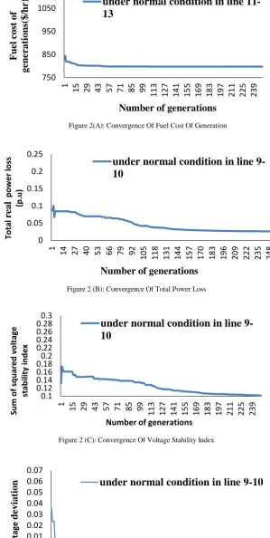
Figures 2(a)-2(d) shows the convergence characteristics of fuel cost of generation, total real power loss, sum of
squared voltage stability index and voltage deviation with SSSC located at different locations of optimal value
under three operating conditions. From these figures it can be observed that the TLBO algorithm reaches the
best solution within 150 iterations under all the operating conditions. Table 5.1shows the OPF results with SSSC
device located in the selected lines with respect to different objective functions. Table 5.1 shows four different
attributes (objectives) such as total fuel cost of generation, total real power loss, sum of squared voltage stability
index and voltage deviation with five different alternatives (different lines)such as 13-7, 11-13, 9-10, 12-14 and
12-16 lines has being taken for SSSC device installation.
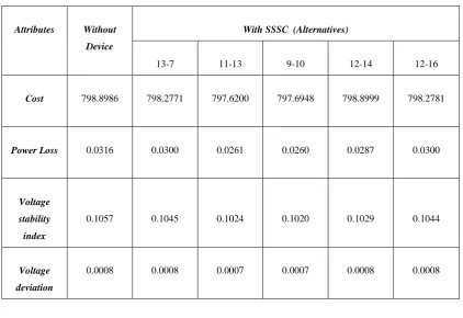
This table also gives that SSSC candidate line 11-13 gives best minimum fuel cost of generation 797.6200$/hr,
SSSC candidate line 9-10 gives best minimum power loss 0.0260p.u, SSSC candidate line 9-10 gives best
minimum sum of squared voltage stability index 0.1020 and best minimum voltage deviation 0.0007in line
11-13 and 9-10 when compared to optimization without device and with SSSC in other alternatives under normal
operation. From the Table 5.1.It can be observed that each candidate bus has given minimum attributes
(objective function value) as best value when compared to optimization without SSSC device.
7.1.2 Case II: Application of MADM methods for determination of optimal location of SSSC
In this section, in order to differentiate the best alternative out of five considered alternatives 13-7, 11-13, 9-10,
12-14 and 12-16 MADM methods are applied. The decision making method considered for determination of
best location of SSSC is AHP. This matrix is based on the preferences given to the four attributes i.e. the pair
wise comparisons determines the preference of each attribute over another. Table 2 also used as priority vector
of the attributes. Priority vector shows relative weights among the attributes that are used for comparison.
Table 1 gives the OPF results with SSSC device is located in the lines with respect to the different objective
functions and is used in decision table for MADM methods. The considered decision matrix of MADM methods
for the system consists of 5 alternatives (different lines)such as 13-7, 11-13, 9-10, 12-14 and 12-16 and 4
www.ijiset.com
314
index and voltage deviation. This decision matrix is given as an input to all the methods. The element in this
matrix indicates the performance of alternative when it is evaluated in terms of decision criterion.
Table 1 Decision Table For MADM Methods
Attributes Without Device
With SSSC (Alternatives)
13-7 11-13 9-10 12-14 12-16
Cost 798.8986 798.2771 797.6200 797.6948 798.8999 798.2781
Power Loss 0.0316 0.0300 0.0261 0.0260 0.0287 0.0300
Voltage stability index
0.1057 0.1045 0.1024 0.1020 0.1029 0.1044
Voltage deviation
0.0008 0.0008 0.0007 0.0007 0.0008 0.0008
Table 2: Relative Ranking Of Alternatives Using AHP Method
Alternatives AHP
13-7 5
11-13 2
9-10 1
12-14 3
12-16 4
As a best choice for the location of SSSC device among the lines considered for the system and this gives
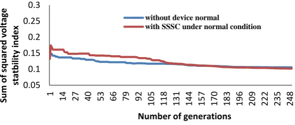
highest benefits to the power system operation in terms of performance parameters. Figure 3(a)-3(d) shows the
convergence characteristics of fuel cost of generation, total real power loss, sum of squared voltage stability
index and voltage deviation with SSSC located in optimal line 9-10.From Figures 5.2(a)-5.3(d), it is observed
that the convergence characteristics of the four objectives obtained are better when compared to without SSSC
315
Figure 2(A): Convergence Of Fuel Cost Of Generation
Figure 2 (B): Convergence Of Total Power Loss
Figure 2 (C): Convergence Of Voltage Stability Index
Figure 2 (d): Convergence of voltage deviation
750 850 950 1050
1 15 29 43 57 71 85 99 113
12 7 14 1 15 5 16 9 18 3 19 7 21 1 22 5 23 9
F
u
el
co
st
o
f
g
en
era
ti
o
n
s(
$
/h
r)
Number of generations
under normal condition in line
11-13
0 0.05 0.1 0.15 0.2 0.251 14 27 40 53 66 79 92
10 5 11 8 13 1 14 4 15 7 17 0 18 3 19 6 20 9 22 2 23 5 24 8 To ta l
rea
l
p ow er lo ss (p .u )Number of generations
under normal condition in line
9-10
0.1 0.12 0.14 0.16 0.180.2 0.22 0.24 0.26 0.280.31 15 29 43 57 71 85 99 113
12 7 14 1 15 5 16 9 18 3 19 7 21 1 22 5 23 9 Su m o f s qu are d vo lta ge st ab ilit y in de x
Number of generations
under normal condition in line
9-10
0 0.01 0.02 0.03 0.04 0.05 0.06 0.071 15 29 43 57 71 85 99
11 3 12 7 14 1 15 5 16 9 18 3 19 7 21 1 22 5 23 9 Vo lta ge
d
evi
at
ion
Number
of
generations
www.ijiset.com
316
Figure 3(a): Convergence of fuel cost of generation of IEEE30 bus system with optimal location of SSSC
Figure 3(b): Convergence of power loss of IEEE 30-bus system with optimal location of SSSC
Figure 3(c): Convergence of voltage stability index of IEEE 30-bus system with optimal location of SSS
750 850 950 1050 1150
1 13 25 37 49 61 73 85 97
10 9 12 1 13 3 14 5 15 7 16 9 18 1 19 3 20 5 21 7 22 9 24 1 Fu el c os t o f gen er at io n( $ /hr )
Number of generations
without device normal condition with SSSC under normal condition
0 0.05 0.1 0.15 0.2 0.25 0.3
1 14 27 40 53 66 79 92
10 5 11 8 13 1 14 4 15 7 17 0 18 3 19 6 20 9 22 2 23 5 24 8 To ta l re al p ow er lo ss (p .u )
Number of generations
without device under normal with SSSC under normal condition
0.05 0.1 0.15 0.2 0.25 0.3
1 14 27 40 53 66 79 92
10 5 11 8 13 1 14 4 15 7 17 0 18 3 19 6 20 9 22 2 23 5 24 8 Su m o f s qu are d vo lta ge st at bilit y in de x
Number of generations
without device normal
with SSSC under normal condition
0 0.01 0.02 0.03 0.04 0.05 0.06 0.07 0.08 0.090.1
1 13 25 37 49 61 73 85 97 109
12 1 13 3 14 5 15 7 16 9 18 1 19 3 20 5 21 7 22 9 24 1 Vv ol ta ge d ev ia tio ns
Number of generations
317
Figure 3(d): convergence of voltage deviations of IEEE 30-bus system with optimal location of SSS
8. Conclusions
In this paper, the TLBO has performed better to solve optimal placement of SSSC for reducing the active power
loss, enhancing voltage stability index, improvement in voltage deviations and reducing the cost. It has been
observed here, that TLBO has the efficiency to reduce the active power loss reasonably without violating any
constraints. Moreover, TLBO owns excellent convergence characteristics. Therefore .from the simulation results
it may be concluded that TLBO is superior to the other algorithms. Simulation results for IEEE 30 bus system
are analyzed and graphs are generated for the optimal placement of SSSC in the transmission line using TLBO
optimization technique based on the AHP method. Graphs are generated for convergence for cost of generator,
power loss, and voltage stability index (VSI) and voltage deviation without and with SSSC FACTS device.
Appendix
OPF-Optimal power flow
SSSC-Static Series Synchronous Compensator
MADM-Multi attribute decision making
AHP-Analytical hierarchy process
TLBO-Teaching learning based optimization
References
[1] Amiri, B. (2012). Application of teaching-learning-based optimization algorithm on cluster analysis. Journal of Basic Applied Science Research, 2(11), 11795-11802.
[2] Babu, B.S., &Palaniswami, S. (2015). Teaching learning based algorithm for OPF with DC link placement problem. International Journal of Electrical Power & Energy Systems, 73, 773-781
[3] 41TSumitVerma41T,41TSubhodipSaha41T, 41TV.Mukherjee41T43TOptimal rescheduling of real power generation for congestion management
using teaching-learning-based optimization algorithm.43T J31TUournal of Electrical Systems and Information TechnologyVolume 5,
Issue 3U31T, December 2018
[4] Bhattacharjee, K., Bhattacharya, A. &Halder, S. (2014). Teaching-learning-based optimization for different economic dispatch problems. ScientiaIranica, 21(3), 870-884.
[5] 31TUhttps://sites.google.com/site/TLBOalgorithm/U31T
[6] Baykasoğlu, A., Hamzadayi, A., &Köse, S.Y. (2014). Testing the performance of teaching-learning based optimization (TLBO) algorithm on combinatorial problems: Flowshop and job shop scheduling cases. Information Sciences, 276(20), 204-218.
[7] Charak, A. (2014). Optimal scheduling of multi-chain hydrothermal system using teaching-learning based optimization. M.Tech. Thesis, Thapar University, Punjab–India.
[8]R. V Rao and VivekPatel . ”An improved teaching- learning – based optimization algorithm for solving unconstrained optimization problems”,ScientiaIranica D (2013) 20 (3), 710-720
[9] FACTS CONTROLLERS IN POWER TRANSMISSION AND DISTRIBUTIONbyK. R. Padiyar.
[10]Understanding FACTS Concepts and Technology ofFlexible AC Transmission SystemsbyNarain G. Hingoranl And Laszlo Gyugyi
www.ijiset.com
318 [12] H. Happ. "Optimal Power Dispatch - A Comprehensive Survey," IEEE Transactions on Power Apparatus and Systems, Vol. PAS-96 (3). pp. 841-854, MaylJune, 1977.
[13] J. Carpentier, Optimal Power Flow, Electric Power and Energy Systems, Vol. 1. No. 1, April 1979, pp. 3-15.
[14] R. C. Burchett, H. H. Happ, D. R. Vierath, and K. A. Wirgau, "Developments in Optimal Power Flow," IEEE Transactions on Power Apparatus and Systems, Vol. PAS-I01 (5). pp. 406-414, February. 1982
[15] B. H. Chowdhury and Rahman, “Recent advances in economic dispatch”, IEEE Trans. Power Syst., no. 5, pp. 1248-1259, 1990
[16] J. A. Momoh, M. E. El-Harwary and RamababuAdapa, “A review of selected optimal power flow literature to 1993, part- I and II”, IEEE Trans. Power Syst., vol. 14, no. 1, pp. 96-111, Feb. 1999.
[17] A. Bhattacharya and P. Chattopadhyay, “Solution of optimal reactive power flow using biogeography-based optimization,”International Journal of Energy and Power Engineering, vol. 3, no. 4, 2010, pp. 269-277.
[18] Enrique Acha, Claudio Esquivel, and Hugo Perez, FACTS Modeling and Simulation in Power Networks. John Wiley and Sons, 2004
[19] Khaled N. Nusair and Muwaffaq I. Alomoush Optimal Reactive Power Dispatch Using Teaching Learning Based Optimization Algorithm with Consideration of FACTS Device “STATCOM”
[20] R. Venkata Rao* Review of applications of TLBO algorithm and a tutorial for beginners to solve the unconstrained and constrained optimization problems
[21] Črepinšek et al. (2012) Presented a note on TLBO algorithm