EPOS

EPOS

K.Werner1_,B.Guiot1,2_,Iu.Karpenko1_,T.Pierog3_,G.Sophys1_,M.Stefaniak1,4

1 _{SUBATECH,UniversityofNantes–IN2P3/CNRS–IMTAtlantique,Nantes,France} 2 _{UniversidadTecnicaFedericoSantaMariayCentro}

Cientifico-TecnologicodeValparaiso,Valparaiso,Chile

3 _{KarlsruheInst.ofTechnology,KIT,CampusNorth,Inst.f.Kernphysik,Germany} 4 _{WarsawUniversityofTechnology,Warsaw,Poland}

Abstract.We summarize the main features of the hadronic interaction model EPOS, which is used for cosmic ray air shower simulations but also for p-p, p-A, and A-A collisions to be compared with experimental data from LHC and RHIC.

1 Introduction

Recent experimental findings required considerable changes in the theoretical understanding of hadronic in-teractions (in particular proton-proton (p-p) scattering). Collective hydrodynamic flow seemed to be well estab-lished in heavy ion (HI) collisions at energies between 200 and 2760 AGeV since a long time, whereas p-p and p-A collisions have often been considered to be simple refer-ence systems, showing “normal” behavior, such that de-viations of HI results with respect to p-p or p-A reveal “new physics”. Surprisingly, the first results from p-Pb at 5 TeV on the transverse momentum dependence of az-imuthal anisotropies and particle yields are very similar to the observations in HI scattering [1, 2].

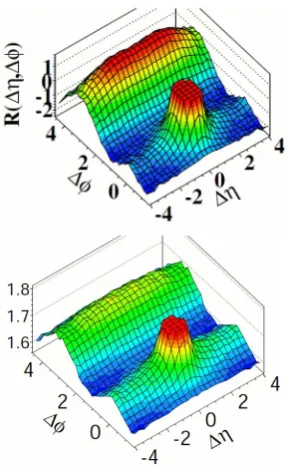
More detailed information about collective flow can be obtained via studying two particle correlations as a func-tion of the pseudorapidity difference∆ηand the azimuthal angle difference∆φ. So-called ridge structures (at∆φ=0, very broad in∆η) have been observed first in heavy ion collisions, later also in pp [3] and very recently in p-Pb col-lisions [4–6], as shown in fig. 1. In the case of heavy ions, these structures appear naturally in models employing a hydrodynamic expansion, in an event-by-event treatment – provided the azimuthal asymmetries are (essentially) lon-gitudinally invariant, as in the string model approach.

To clearly pin down the origin of such structures in small systems, one needs to consider identified particles. In the fluid dynamical scenario, where particles are pro-duced in the local rest frame of fluid cells characterized by transverse velocities, large mass particles (compared to low mass ones) are pushed to higher transverse momenta. These typical “mass effecte” are clearly observed in spec-tra and correlations in HI collisions, but p-Pb results are qualitatively very similar to the Pb-Pb ones.

Figure 1.Two particle correlation functions as a function of the

pseudorapidity difference∆ηand the azimuthal angle difference ∆φ, from the CMS experiment. Upper plot: p, Lower plot: p-Pb. In both cases, the jet peak at∆η=0 and∆φ =0 has been truncated, for better visibility. In both cases a “ridge structure” shows up, at∆φ=0 and very broad in∆η.

In the following, we discuss the EPOS approach, where these “new features” are taken care of.

evolu--2 -1.5

-1 -0.5

0 0.5

1 1.5

2 -1 0

1 2 3 4 1.1

1.2 1.3 1.4

2.0-4.0 GeV/c trigg

T p 1.0-2.0 GeV/c assoc

T p

η

∆

φ

∆

R

EPOS3.074

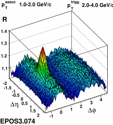
Figure 2. Dihadron correlation function in pPb scattering at 5

TeV, from EPOS simulations.

tion [8–10]. This approach (PBGRT) is the the theoretical basis of the EPOS event generator, or more precisely of the “primary interactions”, happening (at high energies) instantaneously att = 0. We also consider “secondary interactions”, which amounts to a hydrodynamical expan-sion of a core part of matter (determined from the primary scatterings). The EPOS approach uses precisely the same concepts for proton-proton (pp), proton-nucleus (pA) and nucleus-nucleus (AA) scattering.

All EPOS versions, also the most recent ones, are com-posed of primary and secondary interactions, also referred to as initial state and final state scatterings. The former ones are based on PBGRT [7], almost unchanged over the years. The only issue which evolved significantly is the way of treating so-called “high density effects”, referred nowadays as saturation effects. We will discuss this topic in detail.

Also common to all EPOS versions is a core-corona separation mechanism [11], which defines the initial con-ditions of the secondary interactions. This mechanism al-lows to identify a core part which expands collectively, and a corona part of particles escaping from the dense core re-gion. The core part corresponds to a collective evolution of matter. And this collective behavior is present (more or less dominant) in all reactions, from pp to AA. This picture is supported by many experimental LHC results, showing flow-like behavior also for small systems.

Broadening of transverse momentum spectra, and also ridge structures appear naturally in this picture, see Fig. 2. All this discussion about flow in small systems is very interesting, but the main requirement of having a flow-ing medium is a sufficiently high density of strings after the primary scattering stage, and here multiple scattering plays a crucial role. We will therefore in section 2 dis-cuss in detail the multiple scattering approach of primary interactions in EPOS.

Figure 3.Two Pomeron exchange.

+

+ +

Figure 4.Cutting the two Pomeron diagram.

2 Multiple scattering approach of primary

interactions in EPOS

All details of the PBGRT approach, discussed in the fol-lowing, can be found in [7]. LetTbe the elastic (pp, pA, or AA) scattering T-matrix, which means that the total cross section is given as

2sσtot=1

idiscT, (1)

where the discontinuity ofT is defined as discT =T(s+ i,t)−T(s−i). The quantitiessandtare the Mandelstam variables. The basic assumption of PBGRT is the hypothe-sis that the T-matrix can be expressed as a sum of products of elementary objects called Pomerons, in the case of pp scattering (AA is slightly more complicated)

T =

k 1

k!{TPom×...×TPom} (2)

The multiple Pomeron structure must be parallel, as shown in Fig. 3 for the case of two Pomerons, so energy-momentum sharing is an important issue, and Eq. (2) is meant to be symbolic: in reality it contains multidimen-sional integrations over momentum fractions. For the mo-ment the Pomerons are considered to be black boxes (ac-tually the blue and green box in the figure). The next step is the evaluation of the discontinuities (“cuts”),

1

-2 -1.5 -1 -0.5 0 0.5 1 1.5

2 -1 0

1 2 3 4 1.1 1.2 1.3 1.4 2.0-4.0 GeV/c trigg T p 1.0-2.0 GeV/c assoc T p

η

∆

φ

∆

R

EPOS3.074

Figure 2. Dihadron correlation function in pPb scattering at 5

TeV, from EPOS simulations.

tion [8–10]. This approach (PBGRT) is the the theoretical basis of the EPOS event generator, or more precisely of the “primary interactions”, happening (at high energies) instantaneously at t = 0. We also consider “secondary interactions”, which amounts to a hydrodynamical expan-sion of a core part of matter (determined from the primary scatterings). The EPOS approach uses precisely the same concepts for proton-proton (pp), proton-nucleus (pA) and nucleus-nucleus (AA) scattering.

All EPOS versions, also the most recent ones, are com-posed of primary and secondary interactions, also referred to as initial state and final state scatterings. The former ones are based on PBGRT [7], almost unchanged over the years. The only issue which evolved significantly is the way of treating so-called “high density effects”, referred nowadays as saturation effects. We will discuss this topic in detail.

Also common to all EPOS versions is a core-corona separation mechanism [11], which defines the initial con-ditions of the secondary interactions. This mechanism al-lows to identify a core part which expands collectively, and a corona part of particles escaping from the dense core re-gion. The core part corresponds to a collective evolution of matter. And this collective behavior is present (more or less dominant) in all reactions, from pp to AA. This picture is supported by many experimental LHC results, showing flow-like behavior also for small systems.

Broadening of transverse momentum spectra, and also ridge structures appear naturally in this picture, see Fig. 2. All this discussion about flow in small systems is very interesting, but the main requirement of having a flow-ing medium is a sufficiently high density of strings after the primary scattering stage, and here multiple scattering plays a crucial role. We will therefore in section 2 dis-cuss in detail the multiple scattering approach of primary interactions in EPOS.

Figure 3.Two Pomeron exchange.

+

+ +

Figure 4.Cutting the two Pomeron diagram.

2 Multiple scattering approach of primary

interactions in EPOS

All details of the PBGRT approach, discussed in the fol-lowing, can be found in [7]. LetTbe the elastic (pp, pA, or AA) scattering T-matrix, which means that the total cross section is given as

2sσtot=1

idiscT, (1)

where the discontinuity ofT is defined as discT =T(s+ i,t)−T(s−i). The quantitiessandtare the Mandelstam variables. The basic assumption of PBGRT is the hypothe-sis that the T-matrix can be expressed as a sum of products of elementary objects called Pomerons, in the case of pp scattering (AA is slightly more complicated)

T =

k 1

k!{TPom×...×TPom} (2)

The multiple Pomeron structure must be parallel, as shown in Fig. 3 for the case of two Pomerons, so energy-momentum sharing is an important issue, and Eq. (2) is meant to be symbolic: in reality it contains multidimen-sional integrations over momentum fractions. For the mo-ment the Pomerons are considered to be black boxes (ac-tually the blue and green box in the figure). The next step is the evaluation of the discontinuities (“cuts”),

1

idisc{TPom×...×TPom}, (3) which is done using “cutting rules” : A “cut” multi-Pomeron diagram amounts to the sum of all possible cuts,

σ

=

cut P uncut P

A

B

Figure 5.PBGRT formalism: The total cross section expressed

in terms of cut (dashed lines) and uncut (solid lines) Pomerons, for nucleus-nucleus, proton-nucleus, and proton-proton colli-sions. Partial summations allow to obtain exclusive cross sec-tions, the mathematical formulas can be found in [7] or in a some-what simplified form in[12].

as shown in Fig 4 for the example of two Pomerons. Based on these cutting rules, one may express the total cross sec-tion in terms of cut and uncut Pomerons, as sketched in fig. 5. The great advantage of this approach: doing par-tial summations, one obtains expressions for parpar-tial cross sectionsdσexclusive, for particular multiple scattering con-figurations, based on which the Monte Carlo generation of configurations can be done. No additional approximations are needed. The above multiple scattering picture is used for pp, pA, and AA.

The Pomeron is a parton ladder following DGLAP par-ton evolution from both ends, with an elementary hard parton-parton scattering in the middle. It is clear that DGLAP evolution is not enough, in particular when it comes to nuclear collisions. In our approach they will be accommodated via a saturation scaleQs. This is the major improvement of our approach over the past years, so we will discuss this topic in the following.

In our multiple scattering approach PBGRT, we have for each cut Pomeron an expression G = _{2s i}1 discTPom, where TPom represents a parton ladder, computed using the DGLAP equations, using some soft cutoff Q0. The functionsGcan be computed using numerical integration, and their dependence on the light cone momentum frac-tionsx+_andx−_{can be perfectly fitted asG(Q0; x}+_,x−₎₌

α(x+_x−₎β_{,with coefficientsαandβwhich depend onsand} the impact parameterb, and of course on the cutoffQ₀. To mimic nonlinear effects, our fits are modified (for pp) by adding an exponentε, which means instead ofGwe use

Geff(Q0, x+,x−)=α(x+x−)β+ε, (4)

withαandβstill being the above-mentioned coefficient used to fitG. The exponentε =ε(s) is chosen to repro-duce the energy dependence of cross sections. This is the procedure employed in EPOS LHC, which has proven to quite successfully describe LHC data.

Nevertheless, the problem remains that adding an ex-ponentεmust be accompanied by a corresponding modi-fication of the internal structure of the Pomeron, otherwise the whole approach is inconsistent! This can be done by

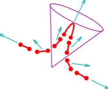
Figure 6.String segments inside and outside the “jet cone”.

defining a saturation scaleQsvia

Geff(Q0; x+,x−)= f ×G(Qs; x+,x−), (5)

(with some coefficient f) and then considering the parton ladder with the cutoffQs, and thus changing the internal structure of the Pomeron.

3 Secondary interactions in EPOS

In heavy ion collisions and also in high multiplicity events in proton-proton and proton-nucleus scattering at very high energies, the density of strings will be so high that the strings cannot decay independently as described above. Here we have to modify the procedure as discussed in the following. The starting point are the flux tubes (kinky strings) representing the cut Pomerons. Some of these flux tubes will constitute bulk matter which thermalizes and ex-pands collectively – this is the so-called “core”. Other seg-ments, being close to the surface or having a large trans-verse momentum, will leave the “bulk matter” and show up as hadrons (including jet-hadrons), this is the so-called “corona”.

In principle the core–corona separation is a dynamical process. However, the knowledge of the initial transverse momenta pt of string segments and their density ρ(x, y) already allows an estimate about the fate of these string segments. By “initial” we mean some early proper time τ0, which is a parameter of the model. String segments constitute bulk matter or escape, depending on their trans-verse momentaptand the local string densityρ. Also low pt segments corresponding to a very high pt jet may es-cape.

Our core-corona separation procedure is based on “jet cones”. We identify for each hard process (in other words for each semihard Pomeron) the primary produced par-tons, and then the string segments corresponding to the same process and being within a cone with respect to the primary parton axis, referred to as “jet cone”, see fig. 6. The jet-cone is defined as

(∆η)2+(∆φ)2 <R2_{, (6)}

central AA

peripheral AA

high mult pp, pA _{low mult pp}

Figure 7.Schematic view of core-corona separation in different

systems. Red dots are core segments, blue ones corona segments.

10-4 10-3 10-2 10-1 1 10 102 103

0 2 4 6

p_t

dn/dp

t

dy

pPb 5TeV 20-40% pions x 100

protons

corona

core

EPOS3.076

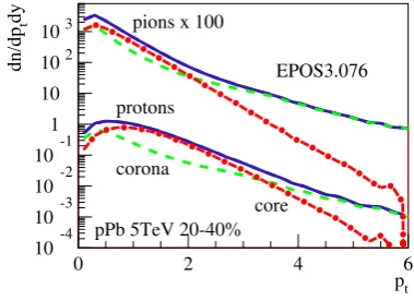
Figure 8.Core and corona contributions.

at initial timeτ0. In the future one may imagine a more sophisticated treatment for the “inside-cone” part, consid-ering the time evolution of the partons in the medium.

We compute for each string segment

pnew

t =pt−fEloss

γ

ρdL, (7)

whereγis the trajectory of the segment. If a segment has a positivepnew

t , it is allowed to escape – it is a corona par-ticle. Otherwise, the segment contributes to the core.

As sketched in fig. 7, we have a nonzero core contri-bution not only in central heavy ion collisions, but even in pp. String segments contributing to the core are shown as red dots, the blue ones represent the corona. The latter ones will show up as hadrons, whereas the core provides the initial condition of a hydrodynamical evolution, where the particles will be produced later at “freeze-out” from the flowing medium, which occurs at some “hadronization temperature”TH. After this “hadronization” the hadrons still interact among each other, realized via a hadronic cascade procedure. For details about hydro evolution and hadronic cascade see [12–14].

In fig. 8, we show how core (red dashed-dotted lines) and corona (green dashed lines) contribute to the produc-tion of pions (upper curves, multiplied by 100) and pro-tons, in semi-peripheral p-Pb collisions at 5 TeV. The blue solid lines are the sum of core and corona. The calcu-lations are done based on the hydrodynamical evolution, without employing a hadronic cascade. The corona contri-butions dominate completely the highptregions. The core

10-1 1 10 102 103

1 10 102 103

<dn_ch/dη(0)>

yield π

EPOS 3.210

full co+co core

Figure 9.The pion production rate as a function of the

multiplic-ity, for pp scattering (thin lines), pPb (normal lines) and PbPb (thick lines), for different contributions. Without the hadronic cascade: From core only (dashed-dotted), from corona only (dot-ted), and the sum of core and corona (co+co) shown as dashed line. The complete simulation, including hadronic cascade (full) is plotted as full line.

becomes important for both pions and protons at interme-diate pt, but the core over corona fraction is much big-ger for protons, and the crossing (core=corona) happens at larger pt. The fact that the core is much more visible in protons compared to pions is a consequence of radial flow: when particles are produced in a radially flowing medium, the heavier particles acquire more transverse momentum than the light ones. It is a mass effect (lambdas look simi-lar to protons, kaons are in between pions and protons).

4 Multiplicity dependence of particle

yields

To test the model for different systems, we compare simu-lations (mainly) to ALICE data [15–23] concerning par-ticle ratios to pions versus multiplicity (more precisely dnch/dη(0)) for different particle species, for minimum bias pp scattering at 7 TeV as well as pPb at 5 TeV and PbPb at 2.76 TeV for different multiplicity bins. Whereas detailed comparisons for different hadrons have been been published [24], we will show here only two examples.

The discussion of these results in the EPOS framework is based very much on the concept of core-corona sepa-ration, as discussed earlier. We therefore show in Fig. 9 the pion production rate at central rapidity as a function of the multiplicity

dη(0)

central AA

peripheral AA

high mult pp, pA _{low mult pp}

Figure 7.Schematic view of core-corona separation in different

systems. Red dots are core segments, blue ones corona segments.

10-4 10-3 10-2 10-1 1 10 102 103

0 2 4 6

p_t

dn/dp

t

dy

pPb 5TeV 20-40% pions x 100

protons

corona

core

EPOS3.076

Figure 8.Core and corona contributions.

at initial timeτ0. In the future one may imagine a more sophisticated treatment for the “inside-cone” part, consid-ering the time evolution of the partons in the medium.

We compute for each string segment

pnew

t =pt− fEloss

γ

ρdL, (7)

whereγis the trajectory of the segment. If a segment has a positivepnew

t , it is allowed to escape – it is a corona par-ticle. Otherwise, the segment contributes to the core.

As sketched in fig. 7, we have a nonzero core contri-bution not only in central heavy ion collisions, but even in pp. String segments contributing to the core are shown as red dots, the blue ones represent the corona. The latter ones will show up as hadrons, whereas the core provides the initial condition of a hydrodynamical evolution, where the particles will be produced later at “freeze-out” from the flowing medium, which occurs at some “hadronization temperature”TH. After this “hadronization” the hadrons still interact among each other, realized via a hadronic cascade procedure. For details about hydro evolution and hadronic cascade see [12–14].

In fig. 8, we show how core (red dashed-dotted lines) and corona (green dashed lines) contribute to the produc-tion of pions (upper curves, multiplied by 100) and pro-tons, in semi-peripheral p-Pb collisions at 5 TeV. The blue solid lines are the sum of core and corona. The calcu-lations are done based on the hydrodynamical evolution, without employing a hadronic cascade. The corona contri-butions dominate completely the highptregions. The core

10-1 1 10 102 103

1 10 102 103

<dn_ch/dη(0)>

yield π

EPOS 3.210

full co+co core

Figure 9.The pion production rate as a function of the

multiplic-ity, for pp scattering (thin lines), pPb (normal lines) and PbPb (thick lines), for different contributions. Without the hadronic cascade: From core only (dashed-dotted), from corona only (dot-ted), and the sum of core and corona (co+co) shown as dashed line. The complete simulation, including hadronic cascade (full) is plotted as full line.

becomes important for both pions and protons at interme-diate pt, but the core over corona fraction is much big-ger for protons, and the crossing (core=corona) happens at larger pt. The fact that the core is much more visible in protons compared to pions is a consequence of radial flow: when particles are produced in a radially flowing medium, the heavier particles acquire more transverse momentum than the light ones. It is a mass effect (lambdas look simi-lar to protons, kaons are in between pions and protons).

4 Multiplicity dependence of particle

yields

To test the model for different systems, we compare simu-lations (mainly) to ALICE data [15–23] concerning par-ticle ratios to pions versus multiplicity (more precisely dnch/dη(0)) for different particle species, for minimum bias pp scattering at 7 TeV as well as pPb at 5 TeV and PbPb at 2.76 TeV for different multiplicity bins. Whereas detailed comparisons for different hadrons have been been published [24], we will show here only two examples.

The discussion of these results in the EPOS framework is based very much on the concept of core-corona sepa-ration, as discussed earlier. We therefore show in Fig. 9 the pion production rate at central rapidity as a function of the multiplicity

dη(0)

as well as pPb (normal lines) and PbPb (thick lines), for different contributions. We first consider results without hadronic cascade: From core only (dashed-dotted), from corona only (dotted), and the sum of core and corona “co+co” shown as dashed line. The complete simulation, including hadronic cascade referred to as a “full” is plot-ted as full line. The curves corresponding to the three col-liding systems (pp, pPb, PbPb) have considerably over-lapping multiplicity ranges. Amazingly, we observe for any of the contributions (full, core, ...) essentially unique

10-2

10-1

1 10 102 103

<dn_ch/dη(0)>

ratio to

π _{ALICE (black)}

p EPOS 3.210 full co+co corona core 10 -4 10-3

1 10 102 103

<dn_ch/dη(0)>

ratio to

π _{ALICE (black)}

Ω EPOS 3.210 full co+co corona core

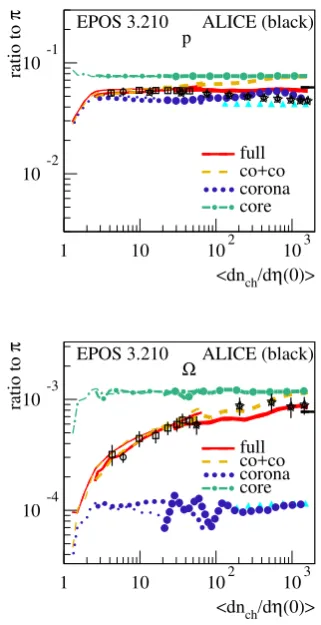
Figure 10. Upper plot: Particle ratios to pions of protons and

antiprotons as a function of multiplicity, as obtained from EPOS simulations, for pp scattering (thin lines), pPb (normal lines) and PbPb (thick lines), for different contributions (as explained in the figure caption of Fig 9). We also show the result from a “pure” EPOS simuation, without hydro and hadronic cascade (triangles). We compare with ALICE data for minimum bias pp scattering (circles) as well as pPb (squares) and PbPb (stars). Lower plot: Same, but for omegas and anti-omegas

curves, so the yields do not depend on the system, but rather on the multiplicity. The yields for pp, pPb, and PbPb agree, as long as the multiplicity is the same. Consid-ering then these unique continuous curves, which extend over the whole multiplicity range, we see that the relative core rate (the core relative to core+corona(co-co) shows a smooth transition from 0% to 100%. Low multiplicity pp is pure corona, high multiplicity PbPb is pure core.

We will now study ratios to pions versus multiplicity and mean transverse momenta versus multiplicity, as ob-tained from EPOS simulations. In Fig. 10 (upper panel), we plot the ratios of protons and antiprotons to pions as a function of multiplicity, as obtained from EPOS simula-tions, for pp scattering (thin lines), pPb (normal lines) and PbPb (thick lines), for different contributions. In addition to the corona contribution, we also show the result from a “pure” EPOS simulation, without hydro and hadronic cascade (triangles). Whereas the origin of both is sim-ply kinky string fragmentation, they are not identical, be-cause the corona particles may suffer energy loss (of the

underlying partons), and the core-corona separation intro-duces biases. Despite this complication, both corona and core contributions are universal curves (pp=pPb=PbPb in the overlap regions), and in addition these two univer-sal curves are flat. Since we know from Fig. 9 that the relative core contribution increases with multiplicity, we understand that the core+corona curve (co+co, dashed) simply interpolates between the corona level at small mul-tiplicity towards the core level at high mulmul-tiplicity. The “full” results shows some reduction with respect to the “co+co” case, with increasing multiplicity, due to baryon-antibaryon annihilation, so at the end the “full” contribu-tion is almost a constant curve. Also shown on the figure as short black horizontal line on the right-hand-side is the result from a statistical model calculation [25].

In Fig. 10 (lower panel), we plot particle ratios to pi-ons of omegas and anti-omegas as a function of multiplic-ity, as obtained from EPOS simulations (same conventions as for the plot on the left). Here again, both corona and core contributions are universal and flat curves (pp=pPb =PbPb in the overlap regions). Again, due to the fact that the relative core contribution increases with multiplicity, we understand that the core+corona curve (co+co, dashed) interpolates between the corona level at small multiplicity towards the core level at high multiplicity. The “full” re-sults shows some reduction with respect to the “co+co” case. The main difference to the proton case of Fig. 10 (upper panel) is the big difference between the corona and the core level (omega production from string decay is very rare), and therefore we get a strong enhancement from low towards high multiplicity.

Apart of protons and omegas, as discussed above, we also studied other hadrons; the results will be summa-rized in the following. Concerning the ratios h/π for h = p,K,Λ,Ξ,Ωversus multiplicity, the core and corona contributions separately are roughly constant, with the dif-ference (core - corona) increasing for p → K → Λ → Ξ → Ω. Since the relative core rate increases with increasing multiplicity, we get monotonically increasing curves for the total contributions, with increasing slopes for p→K→Λ_→Ξ_→Ω.

5 Conclusions

EPOS can explain many experimental curves, concerning basic quantities (not shown) and HI like effects (discussed in this paper), but for the moment still based on different approaches (EPOS LHC, EPOS 3). The “fusion” towards a unique approach, covering all aspects of LHC but also RHIC physics, is the major activity at this moment.

Acknowledgments

This research was carried out within the scope of the GDRE (European Research Group) “Heavy ions at ultra-relativistic energies”.

References

[2] ALICE collaboration, arXiv:1307.6796, Phys. Lett. B 728 (2014) 25-38

[3] CMS collaboration, arXiv:1009.4122, JHEP 1009:091,2010

[4] ALICE collaboration, Phys.Lett. B719 (2013) 29-41, arXiv:1212.2001

[5] CMS collaboration, arXiv:1210.5482, Phys. Lett. B 718 (2013) 795

[6] ATLAS collaboration, arXiv:1303.2084, Phys. Lett. B 725 (2013) 60-78

[7] H.J. Drescher, M. Hladik, S. Ostapchenko, T. Pierog, K. Werner, Phys.Rept. 350 (2001) 93-289.

[8] Yu. L. Dokshitzer, Sov. Phys. JETP 46 (1977) 641 [9] V.N. Gribov and L.N. Lipatov, Sov. J. Nucl. Phys. 15

(1972) 438

[10] G. Altarelli and G. Parisi, Nucl. Phys. B126 (1977) 298

[11] K. Werner, Phys. Rev. Lett. 98, 152301 (2007) [12] K. Werner, B. Guiot, I. Karpenko, and T. Pierog,

Phys.Rev. C89 (2014) 064903, arXiv:1312.1233. [13] Iu. Karpenko, P. Huovinen, M. Bleicher,

arXiv:1312.4160

[14] M. Bleicher et al., J. Phys. G25 (1999) 1859; H. Pe-tersen, J. Steinheimer, G. Burau, M. Bleicher and H. Stocker, Phys. Rev. C78 (2008) 044901

[15] ALICE collaboration, Phys. Rev. C 88 044910 (2013)

[16] ALICE collaboration, Phys. Rev. Lett. 111 222301 (2013)

[17] ALICE collaboration, Phys. Lett. B 728 216–227 (2014)

[18] ALICE collaboration, Phys. Lett. B 728 25-38 (2014)

[19] ALICE collaboration, Eur. Phys. J. C 76 245 (2016) [20] ALICE collaboration, Phys. Lett. B 758 389-401

(2016)

[21] ALICE collaboration, Eur. Phys. J. C 68 345-354 (2010)

[22] ALICE collaboration, Eur. Phys. J. C 75 226 (2015) [23] ALICE collaboration, Phys. Lett. B 712 309 (2012) [24] K. Werner et al, EPJ Web of Conferences Volume