A Fuzzy Replenishment Policy for
Non-instantaneous Deteriorating Inventory
System under Partial Backlogging and Inflation
Effect
D. Chitra , Dr. P.Parvathi
Assistant Professor, Dept. of Maths, Quiad-E-Millath Govt. College for Women(Autonomous), Chennai, India. Head & Associate Professor, Dept. of Maths, Quiad-E-Millath Govt. College for Women(Autonomous), Chennai,
India.
ABSTRACT: This paper explores an Fuzzy inventory model for Non-instantaneous deteriorating items with time varying demand under the effect of inflation. In the proposed model, shortages are allowed and or partially backlogged assuming that backlogging rate varies inversely as the waiting time for the next replenishment. Our goal is to minimize the total Fuzzy cost function with respect to optimal order quantity and optimal interval of the total cost function over a finite planning horizon. All the inventory costs involved here are taken as pentagonal fuzzy number. Graded mean representation method is used to defuzzify the model. The model is illustrated with the help of numerical examples. Sensitivity analysis of the optimal solution with respect to various parameters of the system is carried out and the results are discussed in detail.
KEYWORDS AND PHRASES:Linear time dependent demand, Inflation, Partial backlogging, Non-instantaneous deterioration, pentagonal fuzzy numbers.
I. INTRODUCTION
DETERIORATION plays a significant role in many inventory system. Deterioration is defined as decay, damage, spoilage, evaporation ,obsolescence, pilferage, loss of utility or loss of marginal value of a commodity that results in decrease usefulness. Most physical good undergo decay or deterioration over time, examples being medicines, volatile liquids , blood banks and so on. So decay or deterioration of physical goods in stock is very realistic factor and there is big need to consider this in inventory modeling.
Many researcher assume that the deterioration of an item in an inventory starts from the instant of their arrival in stock. Infact most goods would have span of maintaining quality or original condition.(e.g Vegetables,Fruits,Fish,Meat and so on), namely, during that period there is no deterioration is occurring defined as “non-instantaneous deterioration”. In the real world, this type of phenomenon exist commonly such as first hand vegetables and fruits have short span of maintaining fresh quality, in which there is almost no spoilage. After words, some of the items will start to decay. For this kind of items, the assumption that the deterioration is starts from the instant of arrival in stock may cause retailer to make in appropriate replenishment policies due to over value the total annual relevant inventory cost. Therefore, in the field of inventory management, it is necessary to consider the inventory problems for non-instantaneous deteriorating items.
have a span of maintaining quality or the original condition, for some period. That is during that period there was no deterioration occurring. We term the phenomenon as “non - instantaneous deterioration”. Recently, Wu et.al. [13] developed an inventory model for non-instantaneous deteriorating items with stock–dependent demand.
Furthermore, when the shortages occur, it is assumed that it is either completely backlogged or completely lost. But practically some customers are willing to wait for backorder and others would turn to buy from other sellers.
Researchers such as Park [8], Hollier and Mak [6] and Wee [12] developed inventory models with partial backorders. Goyal and Giri [5] developed production inventory model with shortages partially backlogged.
In all the models mentioned above, the inflation and time value of money were disregarded. It has happened most because of the belief that the inflation and the time value of money would not influence the inventory policy to any significant degree. However, in the last several years most of the countries have suffered from large-scale inflation and sharp decline in the purchasing power of money. As a result, while determining the optimal inventory policy, the effects of inflation and time value of money cannot be ignored. Recently Hou [7] developed an inventory model for deteriorating items with stock dependent demand under inflation. He considered that shortages are completely backordered. R.Udhayakumar et.al have developed a model for Non-instantaneous deteriorating inventory system with partial backlogging.
To fit into realistic circumstances we have developed a finite planning horizon fuzzy inventory model for non-instantaneous deteriorating items with time-dependent consumption rate. In which the Deterioration is a Weibull two parameter distribution and shortages are allowed and partially backlogged. In addition, the effects of inflation and time value of money on replenishment policy under instantaneous replenishment with zero lead-time are also considered. All the inventory cost involved here are taken as pentagonal fuzzy numbers. Graded mean representation method is used for defuzzification. An optimization frame work is presented to derive optimal replenishment policy when the present value of total cost is minimized. Numerical examples are provided to illustrate the optimization procedure. In addition, the sensitivity analysis of the optimal solution with respect to parameters of the system is carried out.
II. FUZZY PRELIMINARIES Definition 1
Let X denotes a universal set. Then the fuzzy subset
A
~
of X is defined by its membership function]
1
,
0
[
:
)
(
~
x
X
A
which assigns a real number ~(
x
)
A
in the interval [0,1], to each element x X where the value of ~(
x
)
A
at x shows the grade of membership of xDefinition 2
A fuzzy set
A
~
on R is convex if ( + (1- for allx
1,
x
2
R
and
[
0
,
1
]
.Definition 3
A fuzzy set in the universe of discourse X is called as a fuzzy number in the universe of discourse X.
Definition 4
A pentagonal fuzzy number (PFN)[9] is represented with membership function
A~As:
e
x
d
x
e
x
L
d
x
c
c
d
x
d
x
R
c
x
c
x
b
b
c
b
x
x
L
b
x
a
a
b
a
x
x
L
x
A
,
)
(
,
)
(
,
1
,
)
(
,
)
(
)
(
1 2 1
~
The a-cut of
A
~
(
a
,
b
,
c
,
d
),
0
a
1
isA
(
)
[
A
L(
),
A
R(
)]
where(
)
(
)
(
)
1 11
a
b
a
L
A
L ,)
(
)
(
)
(
2 12
b
c
b
L
A
L and)
(
)
(
)
(
1 11
d
d
c
R
A
R(
)
(
)
(
)
1 2
2
e
e
d
R
A
RSo
2
)
(
2
)
(
2
)
(
)
(
2
)
(
)
(
)
(
1 2 1
1
1
L
L
a
b
a
b
c
b
a
b
b
a
c
b
a
b
c
a
L
2
)
(
2
)
(
2
)
(
)
(
2
)
(
)
(
)
(
1 2 1
1
1
R
R
d
d
c
e
e
d
d
e
d
c
e
d
d
e
e
c
R
Definition 5:
If is a pentagonal fuzzy number then the graded mean integration representation of
A
~
Is defined as
A A
W W
hdh
dh
h
R
h
L
h
A
P
0 0
1 1
2
)
(
)
(
)
~
(
with0
h
W
A and0
W
A
1
12
3
4
3
2
)
(
2
)
(
2
1
)
~
(
10 1
0
a
b
c
d
e
hdh
dh
h
c
e
e
d
h
a
c
b
a
h
A
P
III. ASSUMPTIONS AND NOTATIONS
The following assumptions are made:
1 . The Consumption rate D(t) at time t is assumed to be
T
t
t
B
t
t
t
t
t
bt
a
t
D
j
j d d
,
,
0
,
)
(
where a is a positive constant, b is the time-dependent consumption rate parameter, 0 ≤ b ≤ 12. The replenishment rate is infinite and lead time is zero.
3. The system operates for a prescribed period of a planning horizon. 4. Shortages are allowed and the backlogged rate is defined to be
)
(
1
1
t
T
when inventory is negative. The backlogging parameter
is a positive constant and5. It is assumed that during certain period of time the product has no deterioration (i.e., fresh product time). After this period, a fraction, θ (0<θ<1), of the n-hand inventory deteriorates according to Weibull two
parameter distribution. i.e.
(
t
)
t
1 is the Weibull tow parameter deterioration where 0<α<1, β>0 are called scale and shape parameter.6. Product transactions are followed by instantaneous cash flow. The following notations are used:
R - r-i, representing the net discount rate of inflation (which is constant.) H - planning horizon.
T - Replenishiment cycle.
M - the number of replenishment during the planning horizon, m=H/T
j
T
-the total time that elapsed up to and including the j
th
replenishment cycle (j=1,2,…,m). where T0=0, T1=T, …, Tm=H.
j
t
-the time at which the inventory level in the jth replenishment cycle drops to zero (j=1,2,…,m).
d
t
- the length of time in which the product has no deterioration (Fresh producj
j
t
T
- time period when shortage occurs (j=1,2,…,m).Q
- the 2
nd, 3rd,…,
m th replenishment lot size
m
I
- maximum Inventory level.b
I
- maximum amount of shortage demand to be backlogged.K
~
- Fuzzy Ordering cost of inventory, $ per order.
t
I
- The inventory level at time t.
- Deterioration rate, a fraction of the on hand inventory, follows weibull two parameter distribution.p
~
- Fuzzy Purchase cost, $ per unith
~
- Fuzzy Holding cost excluding interest charges, $ per unit/ year.s
~
- Fuzzy Shortage cost, $ per unit/year
~
- Fuzzy Opportunity cost due to lost sales, $ per unit
t
T
C
R
T
~
1,
- The Fuzzy average total inventory cost per replenishment.
t
T
TC
DG 1,
- Defuzzified average total inventory cost per unit time.
t
T
C
IV. MODEL FORMULATION
Suppose that the planning horizon H is divided into m equal parts of length T=H/m. Hence the reorder times over the planning horizon H are Tj=jT (j=0,1,2,…,m). When the inventory is positive, demand rate is dependent on linear function of time, whereas for negative inventory, the demand is partially backlogged. The period for which there is no-shortage in each interval [jT,(j+1)T] is a fraction of the scheduling period T and is equal to kT (0<k<1). Shortages occur at time tj=(k+j-1)T, (j=1,2,…,m) and are accumulated until time t=jT (j=1,2,…,m) before they are backordered. This model is illustrated in Fig.1. The first replenishment lot size of Im is replenished at T0=0. During the interval [ 0, t d ], the inventory level decreases due to time-dependent demand rate. The inventory level drops to zero due to time-dependent demand and deterioration during the time interval [t
d , t1]. During the interval [t1, T],
shortages occur and are accumulated until t=T before they are partially backlogged.
I
1
t
denotes the inventorylevel at time t
(
0
t
t
d)
in the product which the product has no deterioration.I
2
t
is the inventory level at timet
(
t
d
t
t
1)
in which the product has no shortage.Therefore the inventory system at any time t can be represented by the following differential equations:
d
t
t
bt
a
dt
t
dI
0
)
(
)
(
1(1)
j d
t
t
t
bt
a
t
I
dt
t
dI
)
(
)
(
)
(
2
2
(2)
T
t
t
t
T
B
dt
t
dI
j
)
(
1
)
(
3
(3)Fig.1 Graphical representation of inventory system
The solutions of the above differential equations after applying the boundary conditions
b
m
I
t
I
t
I
T
I
I
I
1(
0
)
,
2(
1)
0
;
3(
1)
0
,
3(
)
d m
t
t
I
bt
at
t
I
0
2
)
(
2 1
1 2 2 1 2 2 1 2 1 1 1 1 2,
2
)
(
)
(
2
1
)
(
)
(
)
(
t
e
a
t
t
a
t
t
b
t
t
b
t
t
t
t
t
I
t d
(5)
T
t
T
t
t
t
T
B
t
I
3(
)
log
1
1
log
1
1
(6)Considering the continuity of I(t) at t=td it follows that I1(td)=I2(td) which implies that
2
2
)
(
)
(
2
1
)
(
)
(
2 2 2 1 2 2 1 2 1 1 1 1 d d d d d d t mbt
at
t
t
b
t
t
b
t
t
a
t
t
a
e
I
d
(7)At
t
T
the maximum amount of shortage demand to be backlogged during first replenishment cycle is
k
m
H
B
I
b
log
1
1
(8)And also the maximum inventory level during first replenishment cycle are
2
2
2
1
)
)
((
)
(
2 2 2 2 2 2 1 1 d d d d d d t mbt
at
t
m
kH
b
t
m
kH
b
t
m
kH
a
t
m
kH
a
e
I
d
(9)There are m cycles during the planning horizon. Since, inventory is assumed to start and end at zero, an extra replenishment at
T
m
H
is required to satisfy the backorders of the last cycle in the planning horizon. Thereforethere are
m
1
replenishments in the entire planning horizon H. The first replenishment lot size isI
m . The 2nd , 3rd ,…mthreplenishment lot size is
b m
I
I
Q
(10)And the last or (m+1)th replenishment lot size is
I
b Since replenishment in each cycle is done at the start of each cycle, the present value of fuzzy ordering cost/ setup cost during the first cycle is K~Inventory occurs during period
0
t
t
d,t
d
t
t
1 therefore the present value of fuzzy holding costduring the first replenishment cycle is
HC =
33 2 2 2 2 2 2
)
3
(
2
2
2
1
2
d d d Rt d dt
m
kH
b
t
m
kH
a
t
m
kH
a
R
e
bt
at
d (11) Fuzzy Deterioration cost in (0, T1) denoted by DC is given byDC =
1 1
)
(
~
)
(
)
(
~
2 1 2 t t Rt t t Rt d ddt
e
t
I
t
p
dt
e
t
I
t
p
2 22 2 2 1 2 1 2 1 1
)
2
2
(
2
)
1
(
2
1
~
d dt
dm
kH
b
t
m
kH
a
t
m
kH
a
p
(12) The Fuzzy shortage cost in the interval [t1, T) denoted by SC is given bySC =
T t
dt
t
I
s
1)
(
~
3
2~
log[
1
(
)]
(
1
)
1
(
)
m
kH
T
m
H
e
m
kH
T
s
R
B
RmH
(13)The Fuzzy opportunity cost due to lost sales denoted by OC is given by
T tdt
t
T
B
B
OC
11
~
(
1
)
log[
1
(
1
)]
~
k
m
H
k
m
H
B
OC
(14) Fuzzy purchasing cost for the first replenishment cycle is given by
b Rt m
p
e
I
I
p
PC
~
~
2
2
2
1
)
)
((
)
(
~
2 2 2 2 2 2 1 1 d d d d d d tbt
at
t
m
kH
b
t
m
kH
b
t
m
kH
a
t
m
kH
a
e
p
PC
d
k
m
H
B
e
p
RTlog
1
1
~
(15)
Consequently, the present value of fuzzy total cost of system during the first replenishment cycle can be formulated as
T
R
C
K
HC
DC
SC
OC
PC
~
~
(16)
So, the present value of fuzzy total cost of the system over a finite planning horizon
H is RH
m j M RH RH RH RT
Ae
e
e
C
R
T
Ke
Ce
R
T
k
m
C
T
j
1Where T=H/m and
T
R
~
C
is got by substituting the equation 11 to 15 in equation 17 On simplification we get
K
k
m
C
T
~
(
,
)
~
R e bt at t m kH b t m kH b t m kH a t m kH a e R e bt at h d d d Rt d d d d d d t Rt d d 1 2 2 2 1 ) ( 2 ~ 2 2 2 2 2 2 1 1 2
33 2 2 2 2 2
)
3
(
2
2
2
d d dt
m
kH
b
t
m
kH
a
t
m
kH
a
2 2
2 2 2 1 2 1 2 2 1 ) 2 2 ( 2 ) 1 ( 2 1 ~
d d td
m kH b t m kH a t m kH a p
(1 ) log[1 (1 )]
~ ) 1 ( 1 ) 1 ( )] 1 ( 1 log[ ~ 2 k m H k m H B k m H m H e k m H s R B m H R 2 2 2 1 ) ) (( ) ( ~ 2 2 2 2 2 2 1 1 d d d d d d t bt at t m kH b t m kH b t m kH a t m kH a e p d
RHM RH RH RT
e
K
e
e
k
m
H
B
e
p
~
1
1
1
1
log
~
/
Equation (17) is convex with respect to m, k i.e.
0
,
~
m
k
m
C
T
………....(18)and
,
0
~
k
k
m
C
T
………....(19) provided they satisfy the sufficient conditionsand
,
0
~
,
~
,
~
) , ( 2
2
* *
k m at
k
m
k
m
C
T
k
k
m
C
T
m
k
m
C
T
V. NUMERICAL EXAMPLES
To illustrate the preceding theory the following examples are presented.
Example-1:Expressing the fuzzy inventory costs (pentagonal fuzzy numbers) in relevant units. Let
K
~
=(100,150,200,250,300),~
p
=(10,15,20,25,30),h
~
=(1,3,5,7,9),t
d=0.08,~
s
=(5,10,15,20,25),
~
=(8,10,12,14,16),a
=100, b=.09, =0.08, α=0.1, β=2,R
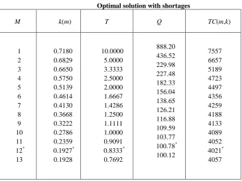
=0.2 B=30, H=10, =.56 From the results presented in Table.1 we see that when the number of replenishment m=12, the total costTC
DG
m
,
k
(defuzzified value) becomes minimum. Hence the optimal values of m and k are m* =12, k*=0.1937 respectively, the minimum defuzzified total cost TCDG(m*,k*),=4021. We then have T*=H/ m*=10/12=0.8333, t1*=k*H/m*=0.1614, Q*=100.78
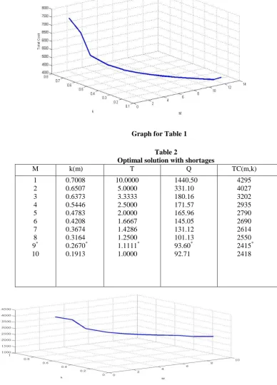
Example-2:Expressing the fuzzy inventory costs (pentagonal fuzzy numbers) in relevant units. Let
K
~
=(200,250,300,350,400),~
p
=(11,13,15,17,19),~
h
=(3,5,7,9,11),t
d=0.08,~
s
=(10,15,20,25,30),
~
=(6,8,10,12,14),a
=80, b=.025, =0.08, α=0.1, β=2,R
=0.2 B=15, =.56, H=10.From the results presented in Table.2 we see that when the number of replenishment m=12, the total cost
m
k
TC
DG,
(defuzzified value) becomes minimum. Hence the optimal values of m and k are m* =9, k*=0.2670 respectively, the minimum defuzzified total cost TCDG(m*, k*)=2415. We then have T*=H/ m*=10/9=1.111,t1*=k*H/m*=0.2966, Q*=93.60.
We now study the effects of changing the parameters θ, R, td and δ on the optimal replenishment policy of the Example 1. The results are summarized in Table 3. Based on Table 3, the observations can be made as follows:
When the deterioration rate θ is increasing, the optimal cost is increasing and the order quantity is decreasing.
When the net discount rate of inflation R is increasing, the optimal cost is decreasing
When the length of fresh product time „ t d ‟ is increasing, the total cost is decreasing And the order quantity is increasing.
When the backlogging rate δ is increasing, the total cost and the order quantity is increasing.
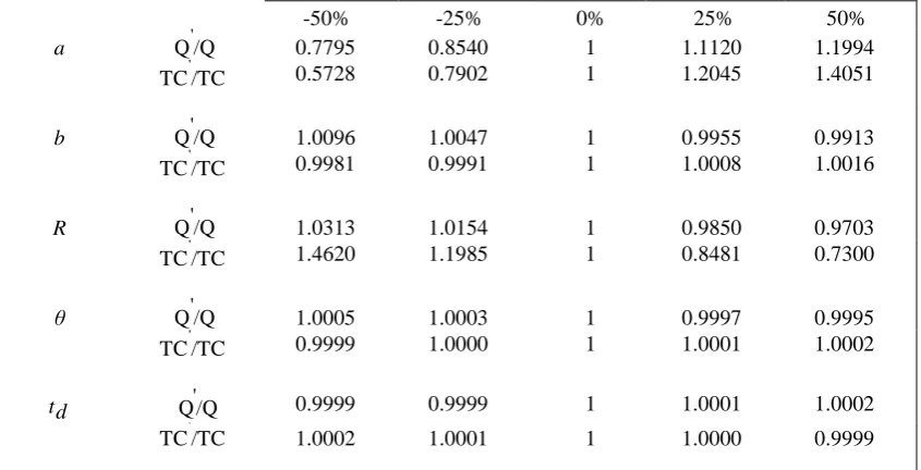
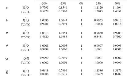
VI. SENSITIVITY ANALYSIS
1. When the consumption rate (a) decreases or increases the ordering quantity (Q) and the present value of total cost (TC) will also decrease or increase. Similarly, the ordering quantity (Q) and the present value of total cost (TC) will also decrease or increase as the ordering cost (A) decrease or increase. That is changes in (a) and (A) will lead to the positive changes in (Q) and (TC).
2. The change in the stock-dependent consumption rate (b) leads to a positive change in the present value of the total cost (TC).
3. The change in net discount rate of inflation (R) leads to a negative change in the present value of total cost (TC).
4. The change in deterioration rate (θ) leads to a negative change on the ordering quantity (Q) and a positive change in the present value of the total cost (TC). That is Q decreases with the increase of (θ).Whereas (TC) increases with the increase of (θ).
5. Increasing the fresh product time ( t d ) increases the order quantity (Q) and decreases the total cost (TC). 6. When the backlogging parameter (δ) increases the ordering quantity (Q) and the present value of total cost
(TC) increases. That is change in (δ) leads to a positive change in (Q) and (TC).
7. Changes in carrying cost (h) and shortage cost (s) result in a positive change in the present value of total cost (TC) and a negative change in the ordering quantity (Q).
8. When the opportunity cost ( π ) increases, the ordering quantity (Q) and the present value of total cost (TC) increases.
9. Change in purchase cost (p) leads to positive change in the present value of total cost(TC) and negative change in the ordering quantity (Q).
10. The present value of total cost (TC) is more sensitive to the consumption rate (a), the unit purchase cost (p) and the net discount rate of inflation (R) as compared to other parameters.
11. Tables 4 and 5 imply that the effect of (R) on (TC) is quite significant for 50% over or under estimation of (R). It implies that the effect of inflation and time value of money on present value of total cost is significant.
Table 1
Optimal solution with shortages
M k(m) T Q TC(m,k)
1 2 3 4 5 6 7 8 9 10 11 12* 13
0.7180 0.6829 0.6650 0.5750 0.5139 0.4614 0.4130 0.3668 0.3222 0.2786 0.2359 0.1927*
0.1928
10.0000 5.0000 3.3333 2.5000 2.0000 1.6667 1.4286 1.2500 1.1111 1.0000 0.9091 0.8333*
0.7692
888.20 436.52 229.98 227.48 182.33 156.04 138.65 126.21 116.88 109.59 103.77 100.78*
100.12
Graph for Table 1
Table 2
Optimal solution with shortages
M k(m) T Q TC(m,k)
1 2 3 4 5 6 7 8 9* 10
0.7008 0.6507 0.6373 0.5446 0.4783 0.4208 0.3674 0.3164 0.2670* 0.1913
10.0000 5.0000 3.3333 2.5000 2.0000 1.6667 1.4286 1.2500 1.1111* 1.0000
1440.50 331.10 180.16 171.57 165.96 145.05 131.12 101.13 93.60* 92.71
4295 4027 3202 2935 2790 2690 2614 2550 2415* 2418
Table 3
Effects of changing the parameter θ, R, td, δ on the optimal replenishment policy
parameter parameter m k T Q TC(m,k) value
θ 0.04 12 0.1901 0.8333 100.14 4009
0.06 12 0.1930 0.8333 100.52 4015
0.08 12 0.1937 0.8333 100.78 4021
0.10 12 0.1934 0.8333 100.80 4023
R 0.10 12 0.2144 0.8333 117.80 8716
0.15 12 0.2044 0.8333 116.40 6243
0.20 12 0.1937 0.8333 100.78 4021
0.25 12 0.1734 0.8333 100.20 3997
td 0.0417 12 0.1913 0.8333 100.70 4025
0.0625 12 0.1926 0.8333 100.74 4023
0.0833 12 0.1937 0.8333 100.78 4021
0.1041 12 0.1952 0.8333 100.84 4019
δ 0.28 9 0.1459 1.1111 98.04 4017
0.42 11 0.0822 0.9091 100.45 4018
0.56 12 0.1937 0.8333 100.48 4021
0.70 13 0.2808 0.7692 120.14 4134
Table 4
Sensitivity analysis for Example 1 with respect to various parameters on order quantity and total cost for Time-dependent consumption rate model.
Parameter Percentage of under estimation and over estimation of parameter
-50% -25% 0% 25% 50%
a Q'/Q 0.7795 0.8540 1 1.1120 1.1994
TC'/TC 0.5728 0.7902 1 1.2045 1.4051
b Q'/Q 1.0096 1.0047 1 0.9955 0.9913
TC'/TC 0.9981 0.9991 1 1.0008 1.0016
R Q'/Q 1.0313 1.0154 1 0.9850 0.9703
TC'/TC 1.4620 1.1985 1 0.8481 0.7300
θ Q'/Q 1.0005 1.0003 1 0.9997 0.9995
K
~
Q '/Q TC'/TC
0.6618 0.8988
0.7996 0.9537
1 1
1.1386 1.0409
1.3179 1.0787
δ Q'/Q 0.5832 0.8396 1 1.0972 1.2710
TC'/TC 0.8291 0.9235 1 1.0638 1.1180
p
~
Q'/Q 1.1881 1.0876 1 0.8162 0.7512
TC'/TC 0.7503 0.8823 1 1.1051 1.1976
h
~
Q'/Q 1.0519 1.0224 1 0.9823 0.9681TC'/TC 0.9940 0.9974 1 1.0021 1.0038
s
~
Q'/Q 1.3242 1.0581 1 0.9453 0.8945
TC'/TC 0.8800 0.9494 1 1.0393 1.0712
~
Q'/Q 0.8200 0.9647 1 1.0354 1.0709 TC'/TC 0.8956 0.9495 1 1.0480 1.0936
Table 5
Sensitivity analysis for Example 2 with respect to various parameters on order quantity and total cost for Time-dependent consumption rate model.
Parameter Percentage of under estimation and over estimation of parameter
-50% -25% 0% 25% 50%
a Q'/Q 0.7795 0.8540 1 1.1120 1.1994
TC'/TC 0.5728 0.7902 1 1.2045 1.4051
b Q'/Q 1.0096 1.0047 1 0.9955 0.9913
TC'/TC 0.9981 0.9991 1 1.0008 1.0016
R Q'/Q 1.0313 1.0154 1 0.9850 0.9703
TC'/TC 1.4620 1.1985 1 0.8481 0.7300
θ Q'/Q 1.0005 1.0003 1 0.9997 0.9995
TC'/TC 0.9999 1.0000 1 1.0001 1.0002 t d Q /Q ' 0.9999 0.9999 1 1.0001 1.0002 TC'/TC 1.0002 1.0001 1 1.0000 0.9999
K
~
Q' /Q TC'/TC
0.6618 0.8988
0.7996 0.9537
1 1
1.1386 1.0409
δ Q'/Q 0.5832 0.8396 1 1.0972 1.2710 TC'/TC 0.8291 0.9235 1 1.0638 1.1180
p
~
Q'/Q 1.1881 1.0876 1 0.8162 0.7512
TC'/TC 0.7503 0.8823 1 1.1051 1.1976
h
~
Q'/Q 1.0519 1.0224 1 0.9823 0.9681TC'/TC 0.9940 0.9974 1 1.0021 1.0038
s
~
Q'/Q 1.3242 1.0581 1 0.9453 0.8945
TC'/TC 0.8800 0.9494 1 1.0393 1.0712
~
Q'/Q 0.8200 0.9647 1 1.0354 1.0709 TC'/TC 0.8956 0.9495 1 1.0480 1.0936
VII. CONCLUSION
In this article, a Fuzzy inventory model has been framed for Non-instantaneous deteriorating items with time-dependent consumption rate over a finite planning horizon. Shortages are allowed and partially backlogged. Further we have considered the effects of inflation and the time value of money in formulating the Fuzzy inventory replenishment policy. Weibull deterioration is considered. All the costs involved in this model are taken as pentagonal Fuzzy numbers and defuzzification by graded mean representation method. Sensitivity analysis with respect to various parameters has been carried out. Our research results implies that, the effect of inflation and time value of money on present value of total cost is more significant and increasing the fresh product time increases the order quantity and decreases the total cost.
Thus, this model incorporates some realistic features that are likely to be associated with some kinds of inventory. The model is very useful in their retail business. It can be used for electronic components, fashionable clothes, domestic goods and other products which are more likely with the characteristics above.
REFERENCES
[1] R.Uthayakumar and K.V.Geetha, A Replenishment policy for Non-instantaneous deteriorating inventory system with partial backlogging,
Tamsi Oxford Journal of Mathematical Sciences 25(3) (2009)313-332.
[2] M. Palanivel, R.Uthayakumar, An EOQ Model for Non-instantaneous deteriorating items with power demand, Time dependent holding
cost, partial backlogging and permissible delay in payments, International Journal of Mathematical, Computational, Statistical, Natural and
physical Engineering Vol:8,No:8,2014.
[3] R. P. Covert and G. C. Philip, An EOQ model for items with weibull distribution deterioration, AIIE Transactions, 5(1973), 323-326.
[4] P. M. Ghare and G. H. Schrader, A model for exponentially decaying inventory system, International Journal of Production Research,
21(1963), 49-46.
[5] S. K. Goyal and B. C. Giri, The production-inventory problem of a product with time varying demand, production and deterioration rates,
European Journal of Operational Research, 147(2003), 549-557.
[6] R. H. Hollier and K. L. Mak, Inventory replenishment policies for deteriorating items in a declining market, International Journal of
Production Economics, 21 (1983), 813-826.
[9] G. C. Philip, A generalized EOQ model for items with weibull distribution, AIIE Transactions, 6(1974), 159-162.
[10] S. Sana, S. K. Goyal, and K. S. Chaudhuri, A production-inventory model for a deteriorating item with trended demand and shortages,
European Journal of Operational Research, 157(2004), 357-371.
[11] Y. K. Shah, An Order-level lot size inventory model for deteriorating items, AIIE Transactions, 9(1977), 108-112.
[12] H. M. Wee, A deterministic lot-size inventory model for deteriorating items with shortages and a declining market, Computers and Operations
Research, 22(1995), 345-356.
[13] K. S. Wu, L. Y. Ouyang, and C. T. Yang, An optimal replenishment policy for non-instantaneous deteriorating items with stock-dependent
demand and partial backlogging, International Journal of Production Economics, 101(2006),369-384.