Modeling multiple time units delayed gene regulatory network using dynamic Bayesian network.

University of Windsor University of Windsor

Scholarship at UWindsor

Scholarship at UWindsor

Electronic Theses and Dissertations Theses, Dissertations, and Major Papers

1-1-2006

Modeling multiple time units delayed gene regulatory network

Modeling multiple time units delayed gene regulatory network

using dynamic Bayesian network.

using dynamic Bayesian network.

University of Windsor

Follow this and additional works at: https://scholar.uwindsor.ca/etd

Recommended Citation Recommended Citation

Xing, Zhengzheng, "Modeling multiple time units delayed gene regulatory network using dynamic Bayesian network." (2006). Electronic Theses and Dissertations. 7147.

https://scholar.uwindsor.ca/etd/7147

M od elin g M u ltip le T im e U n its D elayed G ene

R egu latory N etw ork U sin g D ynam ic B ayesian

N etw ork

by

Zhengzheng Xing

A Thesis

Submitted to the Faculty of Graduate Studies and Research through Computer Science

in Partial Fulfillment of the Requirements for the Degree of Master of Science at the

University of Windsor

Windsor, Ontario, Canada 2006

1 * 1

395 W ellington Street Ottawa ON K 1 A 0N 4 Canada

Bibliotheque et Archives Canada

Direction du

Patrimoine de I'edition

395, rue W ellington Ottawa ON K 1 A 0N 4 Canada

Your file Votre reference ISBN: 978-0-494-42338-7

Our file Notre reference

ISBN: 978-0-494-42338-7

NOTICE:

The author has granted a non­ exclusive license allowing Library and Archives Canada to reproduce, publish, archive, preserve, conserve, communicate to the public by

telecommunication or on the Internet, loan, distribute and sell theses

worldwide, for commercial or non­ commercial purposes, in microform, paper, electronic and/or any other formats.

AVIS:

L'auteur a accorde une licence non exclusive permettant a la Bibliotheque et Archives Canada de reproduire, publier, archiver,

sauvegarder, conserver, transmettre au public par telecommunication ou par I'lnternet, preter, distribuer et vendre des theses partout dans le monde, a des fins commerciales ou autres, sur support microforme, papier, electronique et/ou autres formats.

The author retains copyright ownership and moral rights in this thesis. Neither the thesis nor substantial extracts from it may be printed or otherwise reproduced without the author's permission.

L'auteur conserve la propriete du droit d'auteur et des droits moraux qui protege cette these. Ni la these ni des extraits substantiels de celle-ci ne doivent etre imprimes ou autrement reproduits sans son autorisation.

In compliance with the Canadian Privacy Act some supporting forms may have been removed from this thesis.

While these forms may be included in the document page count,

their removal does not represent any loss of content from the

Conformement a la loi canadienne sur la protection de la vie privee, quelques formulaires secondaires ont ete enleves de cette these.

A bstract

Time delay is an important biological feature of gene regulation, and it is widely observed by biological experiments. Most of the current applications

which use dynamic Bayesian network to model gene regulatory network assume th at the time delay between regulators and their targets is one time unit in a time series gene expression dataset. In fact, multiple time units delay is indicated to exist in the gene regulation process. In this thesis, a method of using higher-order Markov dynamic Bayesian network (HMDBN) to model multiple time units delayed gene regulatory network is proposed. A learning framework using mutual information and genetic algorithm is designed to learn the structure of a HMDBN from time series gene expression data. When applied to real-world yeast cell cycle gene expression datasets, the predicted gene regulatory networks are strongly supported by biological evidence and

Acknowledgm ents

The first person I would like to thank is my supervisor, Dr. Dan Wu. He brought me to the research area of bioinformatics and taught me the way of doing research. When I was frustrated by proposing my own idea about the thesis, his insightful discussions and trust help me out of the hardest time.

Furthermore, he always encourages me to continue my research in the future. Dr. Dan Wu is an excellent supervisor and a good friend to me. I feel fortunate to be his student and finish the thesis under his supervision.

I would like to express my gratitude to my thesis committee members, . Dr. Alioune Ngom, Dr. Andrew Hubberstey, and Dr. Robin Gras. Dr. Alioune Ngom’s excellent courses build me a solid knowledge base in machine learning and computational molecular biology. I was always inspired by his comments during doing the thesis. Dr. Andrew Hubberstey provided me many construc­ tive suggestions on the thesis from a biological point of view. Dr. Robin Gras offered his precious time to be the chair.

Contents

A bstract iii

Acknow ledgm ents iv

List o f Figures vii

List of Tables viii

1 Introduction 1

1.1 Bioinformatics... 1

1.2 Gene Regulatory N etw orks... 2

1.3 Microarray and Gene Expression D a t a ... 6

1.4 Gene Expression A n a ly s is ...10

1.4.1 The First L e v e l...10

1.4.2 The Second L e v e l...11

1.4.3 The Third Level...11

1.5 M otivation...16

1.6 O utline... 17

2 Bayesian N etworks and D ynam ic Bayesian Networks 18 2.1 Bayesian N e tw o rk s ... 18

2.2 Structure Learning of B N s ...21

2.3 First-order Markov Dynamic Bayesian N etw orks... 24

2.4 Structure Learning of First-order Markov D B N s ... 25

3 Learning H M D B N s From G ene Expression D ata 28 3.1 Higher-order Markov Dynamic Bayesian Networks... 28

3.2 A Two Steps Learning Framework...31

CONTENTS CONTENTS

3.2.2 Step 1: Mutual Information M a tr ix ...33

3.2.3 Step 2: Genetic A lgorithm ... 37

3.3 The Problem of Varied Size of Training D a ta ... 42

4 Experim ents 47 4.1 A Nine-Gene Network ... 47

4.1.1 Dataset ...47

4.1.2 R esu lts... 48

4.1.3 Parameter Selection... 56

4.2 A Fourteen-Gene N e tw o rk ...59

4.2.1 Dataset ...59

4.2.2 R e s u l t ... 59

5 Conclusion and Future Work 63 5.1 C o n trib u tio n s... 63

5.2 Future W o rk ...64

Bibliography 65 A ppendix A Source C ode 71 1. A-mean Discretization...71

2. Score. Functions... 74

4. Mutual Information M atrix...76

4. Genetic A lgorithm ... 79

List of Figures

1.1 The process of gene expression... 4 1.2 DNA m ic ro a rra y ... 6 1.3 Collecting gene expression data in cDNA micorarray experiments. 8

2.1 An example of a 5-node Bayesian network...20

2.2 An example of a first-order Markov DBN... 25 2.3 An example of dataset shifting for learning the structure of

first-order Markov DBNs... 26

3.1 An example of a HMDBN...29 3.2 discrete profiles of six yeast genes using k-mean algorithm. . . . 34 3.3 Mutual information matrix for a 2-node 3rd-order Markov DBN. 36 3.4 Crossover for 3-node 3rd-order Markov DBNs... 40 3.5 Knowledge guided mutation for a 2-node 3r<i-order Markov DBN. 42 3.6 Random mutation a 2-node 3rd-order Markov DBN...42 3.7 An example of training data size variation for different HMDBN

structures... 43 3.8 An example of using dataset as a loop... 45

4.1 Gene expression profiles and yeast cell cycle phase information of Chou’s dataset... 48 4.2 Fitness function converging plots for the 9-gene network... 50 4.3 Results Comparison of the 9-gene network using ML score . . . 52 4.4 Results Comparison of the 9-gene network using MDL score. . . 57 4.5 Learning results of r > 5...58

4.6 Fitness function converging plots for the 14-gene network. . . . 60

List o f Tables

1.1 Gene expression d a t a s e t ... 9

3.1 Representation of a network structure in genetic algorithm . . . 39

Chapter 1

Introduction

1.1

B ioinform atics

W ith the completion of sequencing the human genome, the post-genome era

comes. Instead of concentrating on sequencing the genome in a pre-genome

era, now the challenge is to develop efficient methods to harvest the fruits

hidden in the large amount of genomic data. The challenge inspired an emerg­

ing research field, bioinformatics, to appear. Bioinformatics involves biology,

computer science, mathematics, and statistics to analyze genomic data, and

to solve biological problems usually on the molecular level [53]. Besides the

sequence data, many new experimental data produced by modern technolo­

gies, such as gene expression microarray, genetic manipulation of genes in cells

and organisms, are being assembled. The abundance of data offers researchers

a great opportunity to understand the secret of diseases, evolution, biolog­

ical variations, etc. The field of bioinformatics supports a broad spectrum

of research which includes determining the biological significance of the data,

providing the expertise to organize it, and developing practical computational

2 1.2 Gene Regulatory Networks

Currently, the topics in bioinformatics include sequence analysis, computa­

tional evolutionary biology, measuring biodiversity, gene expression analysis,

regulation analysis, protein expression analysis, analysis of mutations in can­

cer, structure prediction, comparative genomics, modeling biological systems,

and high-throughput image analysis [52]. This thesis falls into the areas of

gene expression analysis and regulation analysis.

1.2

G ene R eg u la to ry N etw orks

Deoxyribonucleic acid (DNA) is a nucleic acid that contains the genetic in­

structions specifying the biological development of all cellular forms of life,

and most viruses [1]. A DNA molecule is composed of two strands in the form

of a double helix structure. Each strand is the sequence of combination of four

nucleotides, Adenine (A), Thymine (T), Guanine (G) and Cytosine (C). A is

complementary to T and G is complementary to C, which is also called Watson-

Crick rule [26]. Each nucleotide along one strand of the DNA is matched with

its complimentary nucleotide in the opposite position on the other strand .

Genetic information in DNA is coded in the sequences of nucleotides. The

sequence can be viewed as an instruction book. Using the instruction book,

various proteins can be generated. Protein is a molecular comprising a long

chain of amino acids, which folds into a three-dimensional structure unique to

a particular protein th at has certain biological activities [53]. Every triplet of

nucleotides in a ribo nucleic acid sequence is called a codon. Because there

3 1.2 Gene Regulatory Networks

4 * 4 * 4 = 64. Each codon specify a single amino acid, while a single amino

acid may correspond to several different codons. For example, the amino acid

Lys can be represented by codon AAA or codon AAG. Totally, there are only

20 different amino acids to compose proteins. The set of rules which map a

tri-nucleotide sequences (codon) to an amino acid is also known as the genetic

code. Proteins axe responsible for catalyzing most intracellular chemical reac­

tions (enzymes), for regulating gene expressions (regulatory proteins), and for

determining many features of the structures of cell, tissue, and virus (struc­

tural protein) [27].

A gene is a segment of DNA that specifies a unit of biological functions and

usually corresponds to a protein [53]. In many species, only a small fraction of

DNA appears to be the gene area. The other area of the DNA which has not

been understood to contain genes or have a function is assumed to be the junk

DNA. Genes contain the sequence th at determine the amino acid sequence

of proteins and the surrounding sequences that controls when and where the

protein will be produced [52].

RNA is usually a single-stranded molecule, and similar to DNA, is com­

posed by four nucleotides A, C, G, U. In RNAs, nucleotide U replaces nu­

cleotide T. The complementary rule between nucleotides applies to both RNA

and DNA as A paired with T /U and G paired with C. RNA severs as the

template in the process of converting genes to proteins.

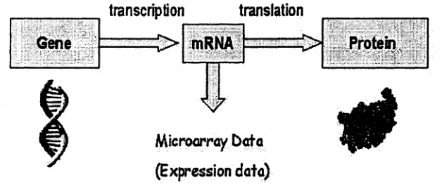
The process of converting the genetic information from DNA into pro­

teins is called gene expression. Gene expression is accomplished by a series of

4 1.2 Gene Regulatory Networks

tion. In the transcription step, a segment of DNA is copied into a messenger

RNA (mRNA). The translation step in gene expression is the synthesis of

proteins from mRNAs. The genetic information flows from DNA to RNA to

proteins, as shown in Figure 1.1, is also known as the central dogma of molec­

ular biology. During the process of gene expression, the amount of mRNA

reflects the degree of genes’ expression. Microarray gene expression data is

obtained by utilizing mRNAs, which is explained in Section 1.3.

Among all the genes in a cell, not all of them are active continuously. In

a particular cell of an organism, at a certain time and under a specific con­

dition, only a subset of genes axe expressed at a high level. The levels of

gene expression may differ from one cell type to another or according to the

stages in the cell cycle. Viewing DNA as the a complex program, then genes

can be seen as functions in the program. The output of every gene function

is a protein. Inside the program, we need a mechanism to call various gene

functions under different conditions. In general, the mechanism th at control

the expression of particular genes in response to external or internal signals is

called gene regulation [27]. Any steps in the process of gene expression may be

regulated, from transcription to post-translational modification of a protein.

transcription

translation

Gene ' ... [>» mRNA C > Protein,

V

Microorray Data (Expression data)

5 1.2 Gene Regulatory Networks

Many genes in eukaryotes are regulated at the level of transcription. Although

both negative and positive regulations occur, positive regulation is typical [27].

In transcriptional regulation, a special protein, called transcription factor,

binds itself to the promoter region of a gene to activate its expression. Be­

cause transcription factors themselves are also the expression products of some

genes, so, they can affect the expression of other genes through their protein

products. The binding site of a gene can be recognized by multiple transcrip­

tion factors, and the expression level of a gene is determined by a combination

of these factors th at bind to the binding site [32]. The regulatory interactions

among genes and proteins form a complex network, called gene regulatory net­

work [26].

Gene regulatory network dynamically regulates the level of expression for

each gene and often includes dynamic feedbacks. Malfunction of gene regu­

latory network is a major cause of human diseases. For example, more than

50 transcription factors have now been identified to be related to human can­

cer [32], Although gene regulatory network is valuable to us, it is still un­

known. A central goal of molecular biology is to understand the regulatory

mechanisms and the synthesis of proteins [19]. Several approaches have been

explored to construct gene regulatory network from available experimental

data. Microarray gene expression data is a major data source th at is used in

6 1.3 Microarray and Gene Expression Data

1.3

M icroarray and G ene E xpression D a ta

A DNA microarray (also commonly known as gene chip, DNA chip, or gene

array) is a collection of microscopic DNA spots attached to a solid surface,

such as glass, plastic or silicon chip forming an array for the purpose of ex­

pression profiling, monitoring expression levels for thousands of genes simul­

taneously [52].

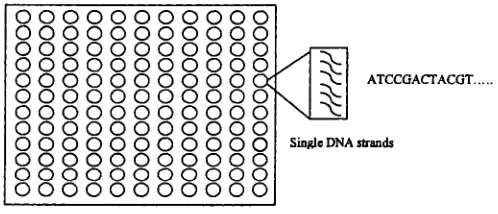
Figure 1.2 is an example of DNA microarray. The spots on the chip axe

arranged in a regular pattern usually forming a rectangular array. Usually,

each spot corresponds to a particular gene, and the specific location of the

spot is used as the identity of a gene. Hybridization is the fundamental basis

of DNA microarray [26]. If two DNA stands are complementary to each other,

they will hybridize to form a double strands union. Hybridization will still

occur when one or both strands of the DNA axe replaced by RNA as long as

they are complementary. Every spot contains many copies of single strand

DNAs (DNA segment) of a particular gene. In microarray experiments, the

spot is used to detect the amount of mRNAs which hybridize with the single

strand DNAs, and the spot is also called probe.

O O O O O O O O O O O O O O O O O O O O O O

ATCCGACTACGT.

O O O O O O O O O O O

O O O O O O O O O O O Single DNA strands

7 1.3 Microarray and Gene Expression Data

There are mainly two kinds of microarray, oligonucleotide microarray (single­

channel microarray) and cDNA microarray (two-channel microarray) [53]. The

basic ideas of the two kinds of arrays are similar. The difference is the way in

which DNA fragments representing the genes are attached to the array.

Oligonucleotides are short sequences of nucleotides (RNA or DNA), typi­

cally with twenty or fewer bases. In oligonucleotide microarrays, the probes

are oligonucleotides, and it is designed to match parts of the sequence of known

or predicted mRNAs. Several companies such as Affymetrix, Healthcare, and

Agilent provide commercial oligonucleaotide microarrays th at cover complete

genomes. These microarrays give estimations of the absolute value of gene

expression. If we have two samples from different conditions, one control sam­

ple and one experimental sample, two separate microarrays need to be used.

Therefore, Oligonucleotides array is also called single-channel microarray.

Complementary DNA (cDNA) microarrays are silimar to the oligonu­

cleotide arrays. Instead of using short oligonucleotides as probes, each spot

contains a cDNA segments clone from a known gene, usually of hundreds of

bases. cDNA is a single stranded DNA synthesized from a mature mRNA

template witch only has exons of genes [53]. cDNA microarray allows multiple

experimental samples, such as control sample and experimental sample, to hy­

bridize at the same time, as long as different dyes are used. Therefore cDNA

microarray is also called two-channel microarray.

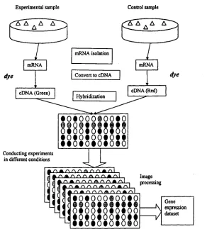
Figure 1.3 depicts the process of using cDNA microarray to collect gene

expression data in a series of experiments. In a single experiment, experi­

8 1.3 Microarray and Gene Expression Data

Experimental sample Control sample

dye dye

mRNA mRNA

cDNA (Red) cDNA (Green)

Hybridization Convert to cDNA mRNA isolation

• 0 « 0 0 0 i 0 0 « 0 9 I 0 9 M I H M

otooioiotoo

• o # o # o o # o # i

• t o t o i o t o i o

in different conditions

ClClO

r \r \r \ r\ r\ Image

processing

• O t O O O i O O t O

o t o o t o e o e o o

• o t o t o o i o f t

• • o t o t o t o t o

expression dataset

Figure 1.3: Collecting gene expression data in cDNA micorarray experiments.

are isolated first. The concentration of a particular mRNA in the sample is a

result of the expression of its corresponding gene. So, the amount of a par­

ticular mRNA is a measure of the expression level of its corresponding gene.

Then, mRNA in the sample is transformed into its cDNA because cDNA is

more stable than mRNA. Experimental and control samples are labeled with

different fluorescent dyes. At last, the two samples are put onto the surface

of a cDNA microarray to let the cDNA in the samples to hybridize with the

probes on the array. Because the microarray chips contains many DNA probes,

when a experimental sample is applied to a chip, different probes will match

dif-9 1.3 Microarray and Gene Expression Data

UID NAME 10 min 30 min 50 min 70 min 80 min 90 min

YAL001C TFC3 -1.04 -0.173 -0.257 -0.617 0.0865 -0.979

YAL002W VPS8 -0.414 0.508 -0.103

YAL003W EFB1 -0.185 -0.039 0.125 0.08 0.655 -0.277

YAL005C SSA1 -1.735 -2.676 -2.865 -3.058 -1.729 -3.262

YAL007C ERP2 0.074 0.61 0.142

YAL008W FUN14 0.394 0.35 0.442 -0.38 0.788 -0.605

YAL009W S P 07 -0.419 0.291 -0.161 0.259 -0.683

YAL010C MDM10 1.585 -0.406 -0.048 -0.023

YAL012W CYS3 -0.289 -0.717 -0.292 0.034 0.879 -0.434

Table 1.1: Gene expression dataset

ferent colors, and the intensity of each spot is related to the expression level

of the particular gene corresponding to th at spot. After an image processing

step , the colors are transformed into gene expression values. Usually, a series

of experiments are conducted under several different experimental conditions,

such as temperatures, times, outside stimulations. A series of experimental

data is organized into a gene expression dataset.

Currently, many gene expression dataset, such as yeast cell cycle gene ex­

pression dataset [6,47], human cell cycle gene expression dataset [51], are

published and can be accessed freely on the Internet. Table 1.1 is an segment

of the gene expression dataset of Spellman et al. [47]. The first two columns

in the table are the IDs and names of genes. Prom the third column, every

column represents the expression levels of all the genes measured at a specific

time in the yeast cell cycle. Every row in the table is the gene expression

profile of a single gene collected in a time series. The blank cells in the table

10 1.4 Gene Expression Analysis

1.4

G ene E xp ression A nalysis

Gene expression data provides a snap shot of the gene expression levels of a

large amount of genes in genome scope and under many different experimen­

tal conditions. It provides us a great opportunity to interpret the underlying

biologcal mechanisms that control the expression of genes. Analyzing gene ex­

pression dataset has become a complete new research area in bioinformatics.

In this section, a literature review on gene expression analysis is provided.

Gene expression data has been analyzed on at least three levels of increas­

ing complexity. First, the level of single genes, where one intends to establish

whether each gene in isolation behaves differently in a control versus a treat­

ment situation. The second level considers gene combinations, where clusters

of genes are analyzed in terms of common functionalities, interactions, co­

regulation, and so forth. The third level is to uncover the gene regulatory

network, or gene regulation pathway [2]. It is the ultimate goal of gene ex­

pression data analysis.

1.4.1 The First Level

In the first level, a mathematical description of the biophysical processes in

terms of a system of coupled differential equations is provided to describe the

processes of transcription factor binding, diffusion, protein and UNA degrada­

tion [4], Constructing differential equations requires detailed understanding of

the interaction agents as well as the parameters of the biochemical reaction.

Therefore, this approach is restricted to describing very small systems [19]. In

11 1.4 Gene Expression Analysis

differential equations are not identifiable when only gene expression data is

observed.

1.4.2 The Second Level

The most popular method in the second level is clustering. The basic idea

of clustering is to group genes into clusters based on the similarities among

their gene expression patterns over different experimental conditions. Genes

in the same cluster are co-expressed. In clustering analysis, it is assumed that

co-expressed genes are co-regulated. Thus, genes in the same cluster may have

similar functions or are involved in related biological processes. Defining the

meaning of similarity is an important issue in all clustering methods. Eisen

et al. [11] first proposed to apply clustering to gene expression data analysis.

Following that, a lot of clustering methods have been designed to group gene

expression data in different ways. D’Haeseleer et al. [8] provided a good survey

of clustering in gene expression analysis. Although clustering provided us a

fast cheap way to extract useful information from a large scale gene expression

dataset, it did not lead to a fine solution of the interaction process. It only

indicates which genes are co-regulated, but in a cluster, whether a gene is the

regulator or the regulatee can not be distinguished [19].

1.4.3 The Third Level

In the third level, it aims to address the ultimate goal of gene expression data

analysis, constructing the gene regulatory network, or gene regulation pathway,

12 1.4 Gene Expression Analysis

from gene expression data can be attacked using two different forms of data:

time series data and steady-state data of gene knockouts [26]. The method

proposed in this thesis belongs to constructing gene regulatory network from

time series gene expression data.

Several machine learning (data mining) methods have been explored to

mine gene regulatory network from gene expression data. Relevance net­

work [3] is constructed by computing comprehensive pair-wise mutual infor­

mation, and then adding undirected edges between gene pairs with a high

mutual information above a threshold. This method can only construct a net­

work structure without directions. Boolean network was first applied to model

gene regulatory network by Liang et al. [30]. In a boolean network model, all

factors in a genetic regulatory network are represented by boolean variables,

which can only take on two possible values, on and off; all relationships be­

tween variables are required to be logical. These restrictions limit the ability

of boolean networks to handle noise data, and to model a gene regulatory

network which can not be represented as exactly logic functions but rather

an inherently stochastic process. Other methods, such as decision tree [29],

neural network [49], have also been applied. In particular, Bayesian network

and dynamic Bayesian network have been proved to be useful tools to model

gene regulatory networks.

Friedman et al. [12] was credited with first proposing and using Bayesian

network (BN) to gene expression analysis. When learning a BN structure

from the gene expression data, they treat each measurement as a sample from

a distribution and do not take into account the temporal aspect of the mea­

13 1.4 Gene Expression Analysis

structure from limited gene expression data efficiently without using any prior

knowledge. When looking for results, they do not use a single best full struc­

ture, but use a bootstrap method to attract the common low dimension net­

work structures from a set of full network structures which all fit the data.

Applied to a yeast time series gene expression dataset containing 800 genes

in 76 measurements, it shows some success in extracting central regulatory

pathways in yeast. This exploration demonstrates the potential of applying

BNs to model gene regulatory networks and also exposes some disadvantages.

One of the important problems is th at although delicate learning algorithm

and bootstrap method are used, the accuracy of predicated relationships is

still very low [38]. It indicated th at the method is not suitable to be applied to

large amount of genes where the predication will become extremely unreliable.

Pe’er et al. [39] extended the framework of Friedman et al. [12] to leaxn a

Bayesian network from perturbed gene expression data. It shows the ability of

BN to handle both time series data and steady-state data with gene mutation

and deletion.

Segal et al. [43] proposed a module network procedure, a method based on

Bayesian network for inferring regulatory modules from gene expression data.

This model is a mixture of Bayesian network and clustering. It is capable

of handling large amount of genes as clustering, and at the same time it can

model a fine structure of gene regulation as Bayesian network.

Unlike Friedman et al., who only use gene expression data, some researchers

explored the possibility to mine knowledge from multiple data sources using

14 1.4 Gene Expression Analysis

the gene expression data but also combining with the location data to enhence

the accuracy of the predicted network structure. Tamada et al. [48] developed

a method to integrate microarray gene expression data and DNA sequence in­

formation into a Bayesian network model. Imoto et al. [22] proposed a method

to add protein-protein interactions, protein-DNA interactions, binding site in­

formation, and existing literature knowledge into BNs.

Usually, gene expression data are discretized into two or three categories

before learning a Bayesian network from the data. Instead of using discreted

variables, a method of using Bayesian network and nonparametric regression

to handle continuous variables was proposed [21].

Although these applications of Bayesian networks can provide some useful

biological information, the dynamic nature of gene regulatory networks was

ignored. Dynamic Bayesian network (DBN), an extension of (static) Bayesian

network to model temporal processes, is more suitable to represent gene reg­

ulatory networks [14]. Furthermore, DBN is not restricted to be an acyclic

graph as BN, which makes it possible to model an important property of gene

regulatory network, the regulatory feedback.

DBN was first introduced to model gene regulatory network by Murphy

et al. [35] and Friedman et al. [14]. In Murphy et al. [35], extracting the dy­

namic interactions among genes from gene expression data was discussed from

a very theoretical point of view. In Friedman et al. [14], a simplified dynamic

Bayesian network was defined and a learning framework for DBNs was pro­

posed. Following that, Ong et al. [37] applied DBN to analyze the regulatory

15 1.4 Gene Expression Analysis

data and continuous variables in dynamic Bayesian network and applied it to

extract gene regulations in DNA repair network of the E.coli [40]. Kim et

al. [24] combined DBN with a non-parametric regression method to construct

nonlinear regulatory relationships from continuous data and tested the method

on a yeast cell cycle gene expression dataset [47]. Zou et al. [55] proposed a

new method to increase the accuracy of prediction of DBN through estimating

the accurate transcriptional time lag.

Although many methods of using BNs or DBNs to model gene regulatory

networks have been developed, evaluating their effectiveness has not been well

studied. Currently, comparing the predicted regulatory network with known

biological knowledge from biological experiments is a widely used method.

This evaluation method lacks of formal standards because of the insufficiency

of current biological knowledge. Some researchers suggested to validate the

methods through simulation studies. Smith et al. [46] designed a simulator to

generate data representing a comlex biological system, and then test various

Bayesian network learning algorithms on the simulated datasets to evaluate

the effectivness. Husmeier et al. [19] proposed a method of using dynamic

Bayesian network and Bayesian learning with Markov chain Monte Carlo to

infer networks from simulated data. In the simulation studies, the issues about

how the network learning performance varies with the size of training data, the

degree of inadequacy of prior assumptions, the experimental sampling strategy

16 1.5 Motivation

1.5

M otivation

In the dynamic process of gene regulation, time delay is an important feature

and is observed by many biological experiments [9]. Time delay could exist in

various situations in a gene regulation process. One of the possibilities is that

one gene is transcribed and translated into a protein, and it then activates or

inhibits its target gene to express. This implies that the expression dependence

between the two genes is not simultaneous, but with a time delay. Dynamic

Bayesian network [15] can model the situation th at one event causes another

event in the future, which makes it suitable to model time delayed gene regu­

latory networks. Although there are some applications of using DBN in gene

regulation analysis [25,35,37,40], in their DBNs, the time delay between all

the regulators and their targets is assumed to be one time unit of a time series

gene expression dataset. Although it was indicated that multiple time units

delay in gene regulation is possible, the computational cost for incorporating

this information into the learning process of DBN is expensive [37]. Zou et

al. [55] proposed an approach to handle multiple time units delay using DBN,

however, the structure of the learned DBN ignored the scenario that several

regulators co-regulate one gene with different time lags. Besides DBN, other

methods, such as decision tree [29], clustering [41] have also been tried to cap­

ture multiple time units delay in gene regulatory networks.

In this thesis, we propose using higher-order Markov DBN (HMDBN) to

model multiple time units delayed gene regulatory networks. A two step heuris­

tic learning framework is designed. First, a mutual information matrix is com­

puted to select gene pairs with a particular time lag as candidate pairs. Then,

17 1.6 Outline

mutual information matrix as prior knowledge. Genetic algorithm interacts

with mutual information m atrix through population initialization and genetic

operators. A particular problem in learning the structure of a HMDBN is

that the size of applicable training data varies when scoring different network

structures. One solution to this problem is suggested in this thesis. In or­

der to verify the effectiveness of the proposed method, we apply the learning

framework to real-life gene expression datasets and compare the results with

biological evidence.

1.6

O utline

This thesis is organized as follows. In Chapter 2, the background of Bayesian

network and dynamic Bayesian network is introduced. In Chapter 3, a new

type of DBN, higher-order Markov DBN is proposed, and the learning frame­

work for it is proposed. The experiments results on Saccharomyces cerevisiae

gene expression datasets are analyzed in Chapter 4. In Chapter 5, the conclu­

Chapter 2

Bayesian Networks and

Dynam ic Bayesian Networks

2.1

B ayesian N etw ork s

Bayesian networks are interpretable and flexible models for representing prob­

abilistic relationships between multiple interacting variables [20]. A Bayesian

network is composed of two components, a graphical component (the structure

of a BN) and a numerical component (the parameters of a BN). At a qualita­

tive level, the structure of a BN describes the relationships between variables

in the form of conditional independence relations. At the quantitative level,

relationships between variables are described by conditional probability dis­

tributions [20]. The two components define a joint probability distributions

over a set of random variables together. In this thesis, we use capital letters

for variable nam es and boldface capital letters for sets of variables. Formally,

considering a set X = {Xt, ...,X n} of random variables, a Bayesian network

(BN) 1 is a graphical representation of a joint probability distribution of X [12].

19 2.1 Bayesian Networks

The graphical structure G of a BN consists of a set of nodes and a set of

directed edges. The nodes represent random variables. The edges indicated

conditional dependence between variables. If there is a directed edge from

node A to node B , then A is called the parent B, and B is called the child of

A. Figure 2.1 is an example of the structure of a five-node Bayesian Network.

In Figure 2.1, we have a set of nodes V = {A, B, C, D, E}, and a set of edges

E = {{E ,B ),{A , B ),(A , D ),{B , C)}. Node E and node A do not have any

parents. Node E and A are the parents of node B. Node D is the child of

node A and node C is the child of node B. The graphical structure of a BN

has to be a directed acyclic graph or DAG, which is defined by the absence of

directed cycles.

The graph G encodes the markov assumption: each variable X , is indepen­

dent of its non-descendant, given its parents in G. This assumption enables a

BN to represent a joint probability distribution of X in a more compact way.

Let X = { X i,..., X„} be a set of random variables represented by the nodes

i = 1, ...n in a BN, and let PA (i) to be the set of parents of variable X*, then,

P ( X l t X 2,....X n) = P(X<|PA(*)). (2.1)

In this way, instead of using a space in the order of 0 (2 n) to present the joint

probability, only a space in the order of 0 (2 fc) is require to represent a Bayesian

network, where k is the maximum number of parents of a variable [34]. Take

Figure 2.1 as an example, according to the markov assumption, variable C is

independent of its non-descendant variables A, E, D given its parent, vari­

20 2.1 Bayesian Networks

I(B ; D\A, E), 1(D) B , C, E\A), and 1(E) A, D). The network structure repre­

sent the joint probability in the form of a production,

P(A , B , C, D, E) = P (A )P (B \A , E )P (C \B )P (D \A )P (E ). (2.2)

The variables in BNs can be continuous or discrete. For discrete variables,

the parameters of BNs are a set of conditional probability tables. Every node is

associated with a conditional probability table given its parents. In Figure 2.1,

every variable can only take boolean values, and the table in the bottom of

the figure is the conditional probability table of variable B. In the table, the

probabilities of all possible assignments of P (B = b\E = e,A = a), where

b, e, a = 0,1 are shown. For continuous variables, the parameters are a set

of conditional probability distribution for every variable. The set of local con­

ditional probability tables or distributions for all the variables, together with

the set of conditional dependence assumptions described by the structure of

the BN, define a full joint probability distribution for the network.

When applying BNs to model gene regulatory networks, we associate nodes

E=I,A*I E=1A=Q E°0,A=1 E*0.A»0

21 2.2 Structure Learning o f BNs

with genes and the values of the nodes with the expression values of genes,

while the directed edges indicates interactions between the genes. For instance,

the network structure of Figure 2.1 suggests that gene E and gene A co-regulate

gene B, th at gene B mediates the interaction between gene E, A and gene C\

that gene A regulate gene D. W ith the parameters of a BN, different type of

regulations, such as inhibition or activation can be differentiated.

2.2

Stru ctu re L earning o f B N s

Learning Bayesian networks from training data can be considered in several

different settings. If the structure of a Bayesian network is known, the task is

to the learn the probability table for each variable from the training data, it

is known as parameters learning; otherwise, the structure needs to be learned

from the training data first, it is known as structure learning. Furthermore,

sometime, not all the the variables in a Bayesian network are observable, some

are not presented in the training dataset or the dataset is not complete, it

involves learning Bayesian network with hidden variables. Below, the basic

idea of learning the structure of BNs from complete dataset is reviewed.

Learning the structure of a (static) Bayesian network from training dataset

can be seen as a search problem to find an optimal structure in the search space

that maximizes a score function. The score function measures the fitness of

a given structure with respect to the dataset. The basic idea of learning the

structure of a BN is to enumerate all the possible structures and choose the one

with the highest score. However, the number of network structures increases

super-exponentially with the number of nodes, and the optimization is a NP-

22 2.2 Structure Learning of BNs

possible structures of the Bayesian network composed by N variables is given

by the formula below,

For n=2, the number of possible structure is 3; for n=3, it is 25; for n=5, it is

29,000; and for n=10, it is approximately 4.2*10(18) [7]. In order to solve the

problem of large search space, heuristic search methods, such as hill-climbing,

simulated annealing, have to be resorted to [17].

Among the existing different score functions, Maximum likelihood (ML) [14]

is a widely used score. It is defined as below [14]:

where N ij.^ is the number of cases in the training dataset when node takes

value ji and its parents take the values A:*. The higher the score for a structure,

the better the structure is.

The problem of ML score is th at it prefers complex structures because

adding more parents to a node can not decrease the likelihood [42]. In order

to find a sparse structure, one solution is to limit the maximal number of

parents. Another solution is to use Minimal description length (MDL) score,

which is proposed to penalize complex structures based on ML score [28]. The

MDL score is defined by the following equations [28,50],

n

(2.3)

1 = 1

23 2.2 Structure Learning o f BNs

M D L — DLdota + DLfnodeii (2-5)

DLtota = -M L , (2.6)

D L m o d e i = [kilog2(n) + d ( 8 i

- 1) n «>].

n i £ n jeFni

where n is the number of nodes ; for node n*, is the number of its parents,

Fni is its set of parents, s, is the number of states it can be in, and Sj is the

number of values a particular variable in Fni can take on; d is the number of

bits needed to store a numerical value. MDL score is the sum of two parts.

The first parts is DLdata, which is used to evaluate how the structure fits the

training dataset. It is in fact the negative ML score. The second part is

D Lm o d e i, which is used to evaluate the complexity of a structure. Because the

structure with lower MDL is better, DLm0<2e* is a penalty for complex structure.

BIC score (Bayesian Information Criterion approximation) [36] is an vari­

ation of MDL score. It is defined as below,

B IC = M L — \ I n M, (2.8)

where d is the number of bits needed to store a numerical value, and M mea­

sures the complexity of the network structure. It is designed for approximation

for large amount of data. Compared to BIC score, MDL is more suitable for

24 2.3 First-order Markov Dynamic Bayesian Networks

2.3

F irst-order M arkov D yn am ic B ayesian N e t­

works

Dynamic Bayesian network (DBN) is an extension of (static) Bayesian network

to model temporal processes [14]. Assuming X = { X i,...,X n} is a set of

attributes changing in a temporal process of T time slices, random variable

Xj[t] denotes the value of attribute at time slice t, and X[t] denotes the set

of variables {Xj[t] | 1 < i < n}, for 0 < t < T — 1. A DBN represents the

joint probability distribution over the variables X[0] (JX[1]... (JX [T — 1] [14].

Because the distribution of a DBN is extremely complex, in [14], a simplified

DBN, called first-order Markov DBN, is proposed based on the following two

assumptions:

1 First Order Markovian:

P ( X [ t ] | X [ t - l ) , X [ t - 2 ] ... X[0]) = P(X[(] | X [t - 1])

2 Stationary: P(X[t] | X[£ — 1]) is independent of t.

First order Markovian assumption means that given variables in X[t — 1], vari­

ables in X[t] are independent of variables in X[t — 2] (JX[£ — 3] | J .... [JX[0].

Stationary assumption means that the dependence between X[t] and X [t—1] is

stationary. This two assumptions together suggest that in a first-order Markov

DBN, arrows are only allowed to appear between adjacent time slices and the

structure between two adjacent time slices remains same as time evolves. Fig­

ure 2.2(a) is an example of a first-order Markov DBN, in which there are three

nodes A, B, C evolving in T time slices. Every node in a particular time

slices represents a variable. Arrows represent probabilistic dependence. In

25 2.4 Structure Learning of First-order Markov DBNs

slices are same. Because of the reduplicate structures, usually, a rolled repre­

sentation which only shows two time slices is used. The rolled representation

of Figure 2.2(a) is shown in Figure 2.2(b). The structure between two time

slices is called inter-slice structure. Applying the structure in Figure 2.2(b) to

model a gene regulatory network, the arrows from node A[t — 1] to C[t) and

from C[t — 1] to C[f] represent th at gene C is co-regulated by gene A and itself

with one time unit delay. It is interesting that DBN can model a regulation

feedback that gene C is regulated by itself.

'a

o

o l 2 T-2 T-l

t-l

(b) Rolled Representa­ tion.

(a) Unrolled Representation.

Figure 2.2: An example of a first-order Markov DBN.

2.4

Structure L earning o f First-order M arkov

D B N s

Learning the structure of a dynamic Bayesian network shares the same idea

with learning the structure of a (static) Bayesian network. Friedman [14] ex­

tended the score functions of BN to evaluate the structure of first-order Markov

DBN. For the structure between two adjacent time slices, the same score func­

tions, such as ML, MDL, for (static) Bayesian network can be used. The

26 2.4 Structure Learning o f First-order Markov DBNs

to be shifted. Given a time series training dataset, to compute the ML score

for a inter-slice structures, N i j ^ has to be counted from the transition cases.

For the first-order Markov DBN, because the parents of a given node are all

from previous adjacent time slice, the transition cases are obtained by shifting

the data of the child one time unit back to align with the data of its parent [34].

10 m 20 m 30 m 40 m SO m 60 m 70 m 80 m 90 m 100 m

A 1 3 2 2 3 2 1 1 3 1

B 1 1 1 3 1 3 1 2 3 1

C 2 2 2 3 3 3 3 1 1 1

(a) A time series gene expression dataset.

10 m 20 m 30 m 40 ra SO m 60 m 70 m 80 m 90 m

B 1 1 1 3 1 3 1 2 3

A 3 2 2 3 2 1 1 3 1

20 m 30 m 40 m SO m 60 m 70 m 80 m 90 m 100 m

(b) Shifted dataset for node A.

10 m 20 m 30 m 40 m SO m 60 m 70 m 80 m 90 m

A 1 3 2 2 3 2 1 1 3

C 2 2 2 3 3 3 3 1 1

C 2 2 3 3 3 3 1 1 1

20 m 30 m 40 m 50 m 60 m 70 m 80 m 90 m 100 m

(c) Shifted dataset for node C.

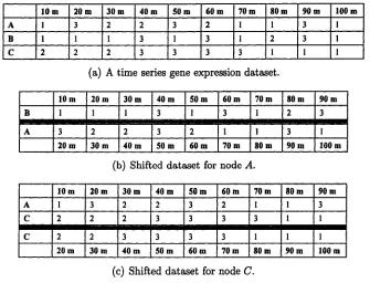
Figure 2.3: An example of dataset shifting for learning the structure of first- order Markov DBNs.

In Figure 2.3, an example of shifting a training dataset to obtain transition

cases is illustrated. Figure 2.3(a) is a gene expression dataset of 3 variables,

gene A ,B ,C . This dataset contains the gene expression of 10 time slices in

a time series from 10 to 100 minute with equal intervals. Given this dataset,

computing the ML score for the structure of a first-order Markov DBN in

Fiure 2.2, the structures of every node given its parents need to be evaluated

27 2.4 Structure Learning o f First-order Markov DBNs

B. To obtain the transition cases where node B affects node A in 10 minutes

later,as shown in Figure 2.3(b), the data of node B from 10 to 90 minute

and the data of node A from 20 to 100 minute is used. Every column in the

shifted dataset is a transition case. For node C, who has two parents, node

A and node C itself from previous time slice, the shifted dataset is shown in

Figure 2.3(c). A transition case is composed by the values of node A and C

Chapter 3

Learning H M D B N s From Gene

Expression D ata

3.1

H igher-order M arkov D yn am ic B ayesian

N etw orks

As suggested in [15], first-order Markov DBN can be extended to allow higher

order interactions among variables. In a rth-order Markov DBN, given a node

Xi[t], its parents can be chosen from the set of varibles X[£ — r] | J |J X[t —

1] [15]. In this thesis, the two assumptions of first-order Markov DBN are

extended for rth-order Markov DBN as below:

1 rth Order Markovian:

P(X[t] I X[i - 1], X[t - 2],..., X[0]) = P(X[i] I X[t - 1],..., X[t - r])

2 Stationary: P(X[£] [ X [t — 1],..., X[f — r]) is independent of t.

r th order Markovian assumption means that given variables X[£—1],..., X [t—r],

29 3.1 Higher-order Markov Dynamic Bayesian Networks

Compared with First order Markowian, it can be seen that variables in time

slice t are dependent on the variables in all r previous time slices instead of

only depending on the variables in time slide t — 1. Stationary assumption

means th at the dependence between X[t] and X[i — 1 ] , X[£ — r] remains the

same when time evolves.

Figure 3.1(a) is an example of an 2nd-order Markov DBN (r = 2). It is

t-2

t-l

t

(a) A 2nd-order Markov DBN.

(b) Compact Representation for the 2nd-order Markov DBN

Figure 3.1: An example of a HMDBN.

represented by 3 time slices in its rolled representation. Generally, a rth-order

Markov DBN can be presented in r + 1 time slice in a rolled representation

because the structures of every r-t-l time slices are identical. In Figure 3.1(a),

there is an arrow from node A in slice t — 2 to node C in slice t. This arrow

is not allowed in a first-order Markov DBN.

Most of the applications using DBN in gene regulation modeling use only

first-order Markov DBNs [25,37,40]. Those applications assume th at all the

30 3.1 Higher-order Markov Dynamic Bayesian Networks

ries gene expression dataset. In fact, multiple time units delay is indicated

to exist in a gene regulation process [9]. Using first-order DBNs to model

gene regulatory networks will ignore some regulation pairs with more than one

time units delay. In the thesis, a method of using rth- order Markov DBN to

model multiple time unit delayed gene regulatory network is proposed. Unlike

first-order Markov DBN, it can model the situation that one gene regulates

another gene with 1,.., r time units delay. For example, if using DBN in Fig­

ure 3.1(a) to model a gene regulatory network, it represents th at gene A and

gene B co-regulate gene C with two time units delay and one time unit delay

respectively; gene B regulates gene A with one time unit delay. The suitable

length of time delay in the scope of 1, ..,r is learned from the gene expression

dataset rather than using a fixed one.

In Figure 3.1(a), imaging an extra arrow from gene B to gene A across two

time slices, then there will be two arrows from gene B to gene A. One is across

two time slices and one is across one time slice. This situation is allowed in

the definition of a 2nd-order Markov DBN. But when using it to model a gene

regulatory network, the situation that gene B regulates gene A with two time

unit delay and one time unit delay simultaneously is hard to be explained. In

the proposed method, using a HMDBN to model a gene regulatory network is

based on the assumption th at one gene can only be the parent of anther gene

with one particular time lag. Based on this assumption, the 2nd-order Markov

DBN in Figure 3.1(a) can be conveniently represented in a compact way as

shown in Figure 3.1(b), in which the arrow from node A to node C attached

with number 2 represents the arrow from node A to node C across two time

31 3.2 A Two Steps Learning framework

Given a time series gene expression dataset of N genes in T time slices, to

learn a r e o rd e r Markov DBN from the dataset is the task of learning a DBN

structure composed by (r + 1 ) x JV nodes. First-order Markov DBN (r = 1) is

the simplest case of learning a structure of 2 x N nodes. When r increases, the

search space becomes extremely larger. Currently, most available time series

gene expression d ata only contains a few dozen time slices. It means the size

of training data is small. The problem of learning an optimal structure from

a large space using limited training data makes learning the structure of a

rth-order Markov DBN (r > 1) an extremely challenging task.

3.2

A T w o S tep s Learning Fram ework

In order to address the problem of large search space, a two steps heuristic

learning framework to learn the structure of a r e o r d e r Markov DBN (r > 1)

is proposed. First, a mutual information matrix is computed to store the

variable pairs with mutual information above threshold m. Second, genetic

algorithm is applied to search for an optimal DBN structure by using the

mutual information matrix obtained in step 1. The learning framework is

presented in Algorithm 1. The details of the framework are described and

explained in the following sections.

3.2.1 Pre-processing: Discretization

Before computing the mutual information and fitness functions, gene expres­

sion data is discretized first. Choosing discrete gene expression values instead

of using continuous ones is because it is more easy to capture the nonlinear

relationships [20]. Some researchers chose fixed threshold to discretize gene

de-32 3.2 A Two Steps Learning Framework

A lgorithm 1 Learning framework____________________________________

Pre-processing-. Discretize the each gene’s expression data in to 3 cate­ gories using k-mean clustering algorithm.

1 Compute mutual information matrix M, select the cells in the matrix

whose values are above threshold m, and update M .

2 Genetic Algorithm (M, r, p, m i, m 2, w, M a x, M ax — fa n — in)

M: Mutual information matrix.

r: the order of the DBN.

p: The size of population.

mi: The percent of population to do knowledge guided mutation.

m2: The percent of population to do random mutation.

w: The percents of the population to do the swap.

Max: The maximal number of iterations.

M ax — fa n — in: The maximal number of parents for a node.

— Initial the population using M and evaluate the population.

— While iterations < M ax

Select:

Choose (1 — w) x p individuals from population probabilisticly

and add it to Population^w.

Crossover: Choose 0.5 x w x p pairs of individual from

population to do the swap and add it to Populationnel£).

K now ledge Guided M utation:

Choose mi x p individuals from populationnew randomly to do knowledge guided mutation.

R andom M utation:

Choose m2 x p individuals from populationnew randomly to do random mutation.

U pdate:

Population *— Populationnew

Evaluate:

Compute fitness function (MDL score, ML score) for

Population

— Return the individual in Population with the lowest MDL score or

33 3.2 A Two Steps Learning Framework

termined according to the overall gene expression data of all the genes in the

dataset. Using the fixed threshold to discretize all the genes is not delicate

enough because the scopes of gene expression value vary for different genes.

Discretizing every gene’s data based on its own expression profile is more rea­

sonable. In the thesis, a discretization method using k-mean algorithm [10]

to group every gene’s expression values into three clusters is proposed. Given

one gene’s expression profile composed by n values, the initial means of the

three clusters are the lowest, average and highest values of the n values. Every

value in the profile is then assigned to the closest cluster and the means of the

three clusters are updated. This process is repeated until the the means of the

three clusters are stable. Using clustering to discretize gene expression data

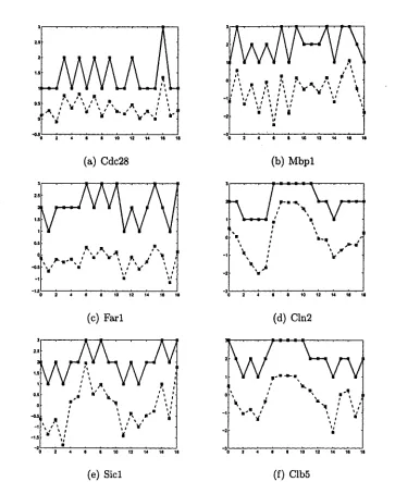
was also adopted in Pe’er et al. [39]. Figure 3.2 shows the discretization results

of 6 genes’ expression profiles in Spellman’s dataset. The horizon axis is the

time points and the vertical axis is the gene expression values. The profile in

dashed line is the original gene expression values and the profile in solid line is

the discrete values as 1,2,3. Figure 3.2 shows that the shapes of the discrete

profiles are similar to the original ones, and most of the turning points are

kept.

3.2.2

Step 1: M utual Information Matrix

Mutual Information [3] is a natural way to measure the dependence between

two variables and was employed in gene expression analysis [3,12]. It is defined

where X , Y are two variables, x, y are particular values that X , and Y take, by as [13],

P (x)P (yy (3-1)

34 3.2 A Two Steps Learning Framework

(a) Cdc28

(c) Farl

(e) Sicl

(b) Mbpl

(d) Cln2

(f) Clb5

35 3.2 A Two Steps Learning Framework

information, the stronger the dependence between X and Y .

To learn a r t/l-order DBN of N variables evolving in time series, a matrix M

with the dimension of N x N x r is computed first. The cell M(i , j, I), where

1 < j < N, 1 < I < r , is the mutual information between variable X j and

Xi with time lag I (X j precedes X {). When computing the mutual information

I), the data of X t needs to be shifted back I time units to align with the

data of X j [18]. The value of threshold m is set to select the candidate pairs

with a mutual information above the threshold. In the proposed method, m is

chosen as the mean of the overall mutual information. The matrix M is then

transformed to record the candidate pairs with particular time lags using the

following Equation,

) = I represents X j and Xi with time lag I has a high mutual infor­

mation; while M ( i , j , l) = —1 represents the mutual information is low. When

searching DBN structures, if ) = I, it is more likely th at there will be

an arrow from variables Xj[t — /] to variable Aj[£]. That is to say, variable

Xj[t — /] is a good candidate parent for variable X i[f]. The same idea was also

employed in Sparse candidate algorithm [13].

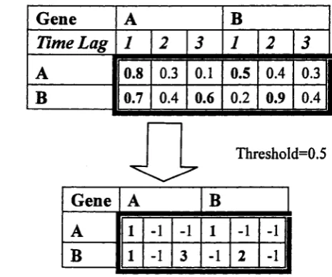
Figure 3.3 is an example of computing mutual information matrix for a

2-node 3rd-order Markov DBN. A matrix of dimension of 2 x 2 x 3 is first

computed to store the mutual information between variable A and B with time

36 3.2 A Two Steps Learning Framework

is

0.8 + 0.3 + 0.1 -F 0.5 + 0.4 -F 0.3 -F 0.7 -F 0.4 -F 0.6 -F 0.2 -F 0.9 -F 0.4

---— -— --- « 0.5.

2 * 2 * 3

(3.3)

Then, 0.5 is used as the threshold to transform the mutual information matrix

to store good candidate parents for every node. In the matrix at the bottom,

in the intersection of column A and row B, the numbers 1, —1,3 represents it

is more possible th at there is an arrow from gene A to gene B with time lag 1

or time lag 3.

G e n e

A

Time Lag 1

2

3

1

2

3

A

0.8

0.3

0.1

0.5

0.4

0.3

II

B

0.7

0.4

0.6

0.2

0.9

0.4

I

Threshold=0.5

G e n e

A

A

1 -1

-1

1

-1

-1

B

1 -1

3

-1

2

-1

Figure 3.3: Mutual information matrix for a 2-node 3rd-order Markov DBN.

Zou et al. [55] proposed a method to find good candidate parents for a

gene with a particular time lag. In their method, given a time series gene

expression dataset, in order to determine if gene A is a possible parent of gene

B, a threshold is chosen to determine the time point of the initial significant

change in the expression profiles of gene A and B. If gene A’s significant initial

change is before gene B ’s, then gene A is chosen as a good candidate parent of