Using bayesian networks to construct gene regulatory networks from microarray data

(1)

58 (2012) 1–6 | www.jurnalteknologi.utm.my | eISSN 2180–3722 | ISSN 0127–9696

Full paper

Jurnal

Teknologi

Using

Bayesian

Networks

to

Construct

Gene

Regulatory

Networks

from

Microarray

Data

Tan Ai Kunga, Mohd Saberi Mohamada*

a

Faculty of Computer Science and Information System, Universiti Teknologi Malaysia, 81310 UTM Johor Bahru

*Corresponding author: [email protected]

Article history

Received: 20 September 2011 Received in revised form: 5 March 2012

Accepted: 2 April 2012

Graphical abstract

Abstract

In this research, Bayesian network is proposed as the model to construct gene regulatory networks from

Saccharomyces cerevisiae cell-cycle gene expression dataset and Escherichia coli dataset due to its

capability of handling microarray datasets with missing values. The goal of this research is to study and to understand the framework of the Bayesian networks, and then to construct gene regulatory networks from

Saccharomyces cerevisiae cell-cycle gene expression dataset and Escherichia coli dataset by developing

Bayesian networks using hill-climbing algorithm and Efron’s bootstrap approach and then the performance of the constructed gene networks of Saccharomyces cerevisiae are evaluated and are

compared with the previously constructed sub-networks by Dejori [14]. At the end of this research, the gene networks constructed for Saccharomyces cerevisiae not only have achieved high True Positive Rate (more than 90%), but the networks constructed also have discovered more potential interactions between genes. Therefore, it can be concluded that the performance of the gene regulatory networks constructed using Bayesian networks in this research is proved to be better because it can reveal more gene relationships.

Keywords: Bayesian networks; gene regulatory networks; interactions between genes

Abstrak

Dalam penyelidikan ini, Bayesian network adalah dicadangkan sebagai model untuk membina gene regulatory networks dari kitar sel S. cerevisiae set data disebabkan keupayaannya untuk mengendali set

data microarray yang mempunyai nilai-nilai yang hilang. Tujuan penyelidikan ini adalah untuk

mempelajari dan memahami rekabentuk untuk Bayesian network, dan kemudian untuk membina gene regulatory networks dari data Saccharomyces cerevisiae cell-cycle gene expression dan data Escherichia coli dengan membina model Bayesian networks dengan menggunakan algoritma hill-climbing serta

Efron’s bootstrap approach dan gene networks yang dibina untuk Saccharomyces cerevisiae

dibandingkan dengan sub-networks yang dibina oleh Dejori [14]. Pada akhir kajian ini, gene networks

yang dibina untuk Saccharomyces cerevisiae bukan sahaja telah mencapai True Positive Rate yang tinggi (lebih dari 90%), tetapi gene networks yang dibina juga telah menemui lebih banyak interaksi berpotensi antara gen. Oleh kerana itu, dapat disimpulkan bahawa prestasi gene networks yang dibina menggunakan

Bayesian network dalam kajian ini adalah terbukti lebih baik kerana ia boleh mendedahkan lebih banyak

hubungan antara gen.

Kata kunci: Bayesian network; gene regulatory networks; interaksi berpotensi antara gen

1.0 INTRODUCTION

Microarray technologies have produced tremendous amounts of gene expression data in the recent years [1]. Mining these microarray data to understand the gene expression and gene regulation brings a major challenge in bioinformatics field. The major focus on microarray data analysis is the reconstruction of gene regulatory network (GRN), which aims to discover the

underlying network of interactions between genes from the measured dataset of gene expression [2–3].

Gene regulatory networks are also known as genetic regulatory

(2)

The edges (links) of the network graph represent the interactions between any pair of genes.

In the past few years, many algorithms have been proposed

and developed to infer and to construct gene regulatory networks from microarray data. However, most of the algorithms proposed are still have their own different limitations and weaknesses.

According to Bansal et al. [5], clustering algorithm is the current

choice to visualize and to analyze gene expression data. Clustering algorithm is developed based on the idea of grouping genes with similar expression profiles into clusters [6]. However, clustering is not a proper network inference algorithm because it can only be used to construct undirected network graph.

Besides that, Boolean network has also been used in

constructing gene networks. According to Huang [7], Boolean networks have proved successful in modeling real world regulatory networks. However, several weaknesses still exist with the application. For example, analysis can be problematic due to the exponential growth in Boolean states and the lack of tool supports in this area. Besides that, they are also unable to handle incomplete regulatory network data that occur in practice frequently.

Other than that, ordinary differential equations (ODEs) have

been widely used as well to model gene regulatory networks. Gene regulatory network model based on ordinary differential equations (ODEs) relate the changes in gene transcript concentration to each other and to an external perturbation. Advantages of ODEs-based model including it can produce signed directed graphs and can be applied to both steady-state and time-series expression profiles. However, finding appropriate parameter values that fit with the data is very difficult and this is the model’s greatest weakness. Therefore, this approach is restricted to very small systems.

Recently, Bayesian networks have been widely used to analyze

expression data [8]. According to Steele et al. [9], Bayesian

networks are graph-based model of probability distributions that is capable to capture the properties of conditional independence between variables. The expression levels of genes are represented by the nodes in the network graph and dependencies between genes are represented by the directed edges in gene regulatory network modeling.

Compared with other algorithms, Bayesian networks have the

ability of uncovering independency among genes which helps to study the interaction of gene regulation. Besides that, Bayesian networks also have the ability of handling noisy and uncertainty in microarray dataset which contains missing values. Other than that, Bayesian networks are also capable to handle large scale of DNA microarray data, which is very crucial in gene regulatory network construction. Therefore, in this paper, Bayesian networks have been used for gene regulatory networks construction from

Saccharomyces cerevisiae cell-cycle gene expression dataset by

Spellman et al. [10].

2.0 MATERIALS AND METHODS

2.1 Impute Missing Values

In order to prepare a complete database for constructing Bayesian networks, the missing data in microarray datasets have to be imputed. Therefore, Least Local Squares (LLSimpute), an

imputing algorithm that is developed by Kim et al. [11] is chosen

and it is used to estimate the missing values in target genes. LLSimpute algorithm estimates the missing values in the target

genes as the linear combination of their most k-similar neighbours

chosen by the first k smallest Euclidean distance. Assume that the

target gene contains a missing value in the first position of its

total n = 5 experiment measures, k similar genes are chosen,

which consists of complete measurements before imputing the

missing value into the target gene. Then, matrix A, vectors b and

w, and the missing value are constructed as follows:

, , , ,

(1)

where α represents the missing value in ,

contains n - 1 elements of whose first missing item is deleted.

The elements of b are the first components of the

k-nearest genes. Then, the rows of the matrix A which contain

k-nearest neighbour genes with their first values are deleted. With

the above definition, the missing value α can be estimated as a

linear combination of the vector b:

(2)

where is the pseudoinverse of . All these procedures are

implemented in LLSimpute function.

However, if a gene misses too many values across the entire

microarray experiments, LLSimpute algorithm will not be able to estimate a coefficient for these missing data. Therefore, an imputing algorithm known as FinalImpute is implemented to impute too bad data into a specified value, which means the expression levels of the gene cannot be detected in these experiments.

2.2 Construct Bayesian Networks

According to Bansal et al. [5], Bayesian networks can be

explained as graphical models for probabilistic relationships

among a set of random variables , where i = 1 … n. the

probabilistic relationships are represented in the structure of a

directed acyclic graph G. The vertices (nodes) are the random

variables . Then, the relationships between the variables can be

explained by using a joint probability distribution P( , … , ).

The joint probability distribution is consistent with the

independence assertions embedded within the graph G. It can be

represented in the following form:

, … , ∏ || , … , (3)

where the p + 1 genes are known as the parents of gene i on which

the probability is conditioned. By applying the chain rule of probabilities and independence, the joint probability density is expressed as a product of conditional probabilities. The chain rules are based on the Bayes theorem as below:

, || || (4)

The joint probability distribution can be decomposed as the

product of conditional probabilities only if the Markov assumptions hold. The Markov assumptions stated that each variable is independent of its non-descendants, given its parent

is in the directed acyclic graph G.

In this research, Bayesian networks are used to construct gene

regulatory networks from microarray data. After the missing values in microarray dataset are imputed by using LLSimpute

algorithm, an R package bnlearn is implemented to learn

Bayesian networks from the data.

R package bnlearn includes several algorithms for learning the

(3)

variables. Both constraint-based and score-based algorithms are implemented within the package. Constraint-based algorithms are algorithms that learn the network structure by analyzing the probabilistic relations entailed by the Markov property of Bayesian networks with conditional independence tests and then constructing a graph which satisfies the corresponding d-separation statements. The resulting models are often interpreted as causal models even when learned from observational data [12].

On the other hand, score-based algorithms are algorithms that

assign a score to each candidate Bayesian network and try to maximize it with some heuristic search algorithm. Hill-Climbing (hc) is the only available score-based learning algorithm in the package which performs greedy search on the space of directed graphs. One of the advantages of using hill-climbing is that it can be used in almost any kind of search procedure. Besides that, according to Marco [13], the network structure learned by constraint-based algorithms is equivalent to the one learned by hill-climbing.

Therefore, due to the several advantages mentioned earlier,

hill-climbing algorithm is selected and is implemented in this research to learn Bayesian network. Finally, an optimized Bayesian network is obtained by using the hill-climbing algorithm

from bnlearn R package. The obtained network structure encodes

the conditional independence relationship among the genes in the domain.

2.3 Bootstrap Bayesian Networks

In order to fully make use of the limited experiment data as far as possible, several best reasonable Bayesian networks are generated from the microarray data by using Efron’s non-parametric bootstrap approach with replacement. This method provides a computationally effective approach to estimate the confidence levels on features of generated networks.

Then, by choosing edges whose confidence levels exceed the

pre-defined threshold, a set of highly confident edges are obtained whose encoding relationships are believable. Furthermore, the bootstrap produced Bayesian networks are then used to construct gene regulatory network. This step is implemented by using BootstrapBN function in the package. The constructed Bayesian networks are then stored in matrix form by using WriteBootBN function in the package.

2.4 Construct Gene Regulatory Network

Based on the matrix form of Bayesian networks that are constructed using bootstrap approach earlier, a gene regulatory network in matrix form is constructed by using CalcEdgeSup function. Then, the gene regulatory network constructed is

displayed in graph form using R package Rgraphviz and R

package graph, which can be downloaded from

http://www.bioconductor.org/.

Both R package Rgraphviz and R package graph are able to

display nodes and edges in a network clearly without having the nodes overlapping with one and another. Besides that, both packages are also capable to display regulatory network with huge

amount of genes (nodes). Hence, this is why R package Rgraphviz

and R package graph are implemented in this research to visualize

gene regulatory network constructed.

3.0 RESULTS AND DISCUSSION

3.1 Dataset and Experimental Setup

For this research, two microarray datasets are selected to be used to construct gene regulatory networks for further analysis. The

selected microarray datasets are Saccharomyces cerevisiae dataset

and Escherichia coli dataset.

The Saccharomyces cerevisiae dataset chosen is the cell-cycle

gene expression dataset by Spellman et al. [10]. Saccharomyces

cerevisiae is selected because it is widely available and contains

less noise. Besides that, the dataset is available in a text file format and can be easily downloaded from http://www.cls.zju.edu.cn/binfo/BNArray/. The dataset consists of 6178 genes in total and 78 expression measurements. However, only 800 differentially expressed genes are selected for further gene network modelling.

The Escherichia coli dataset chosen is the Escherichia coli

whereby the expression levels of the genes are measured by using

Affymetrix GeneChips. The dataset file is available freely to the public and can be downloaded in a text file format from http://cybert.microarray.ics.uci.edu/datasets/. The file contains 4241 genes in total and 12 expression measurements.

Firstly, LLSimpute algorithm is applied to impute missing

values in the genes. These genes are then being used to construct

Bayesian network by using an R package bnlearn. From bnlearn,

hill-climbing algorithm is selected and is implemented in this research to learn Bayesian network. After that, the microarray data are bootstrapped 3 times by using Efron’s non-parametric bootstrap approach to produce 3 best reasonable Bayesian networks. Next, a gene regulatory network in matrix form is constructed by using CalcEdgeSup function and is displayed

using Rgraphviz R package.

3.2 Results and Discussion

Overall, this section is divided into two parts for two different datasets. Firstly, the gene networks constructed for

Saccharomyces cerevisiae dataset are displayed and compared

with the sub-networks constructed by Dejori [14]. After that, gene

networks for Escherichia coli dataset are displayed and explained

generally.

3.2.1 Saccharomyces cerevisiae

The gene networks constructed for Saccharomyces cerevisiae

dataset in this research are compared with the sub-networks produced by Dejori [14]. The research done by Dejori [14] is implemented in Java and he has implemented Bayesian network to construct gene networks which is also being implemented in this research. Besides that, the research done by Dejori [14] also

has used Saccharomyces cerevisiae cell-cycle gene expression

dataset by Spellman et al. (1998) as the dataset, which is the same

for this research.

Therefore, the sub-networks constructed by Dejori [14] are the

benchmarks for this research’s networks. The sub-networks that are chosen to be compared are YOR263C sub-network and YPL256C sub-network. True Positive (TP), True Negative (TN), False Positive (FP), and False Negative (FN) are calculated to evaluate the performance of the sub-networks constructed from the research.

Figure 2.0 shows the YOR263C sub-network that is

(4)

to each other on the DNA strand of chromosome XV. However, the biological and molecular functions for both genes are unknown still.

Another feature with high confidence level is the undirected

edge between YNR067C and YGL028C. The function of YNR067C is still unknown currently. The function of YGL028C is known to be a soluble cell wall protein. It has an undirected edge with YER124C, but the function of YER124C is unknown. Gene YGL028C is also related to YLR286C, an endochitinase that is involved in cell wall biogenesis. These two nodes (genes) are again connected by an undirected edge of high confidence.

Since YER124C had undirected edge with two nodes

(YLR286C, YGL028C) and both nodes are functionally related to cell wall biogenesis, therefore, it can be assumed that it is also involved in cell wall biogenesis. Therefore, this gene network constructed using Bayesian networks have provided a testable prediction of an unknown gene function.

Figure 2.0 YOR263C sub-network constructed by Dejori [14]

Figure 2.1 shows the YOR263C sub-network that is

constructed in this research. The constructed network consists of 8 nodes (genes) and 10 directed edges. The main difference between the sub-networks constructed by Dejori [14] with this research is that the edges in the network constructed in this research are directed, whereby they can show the interactions between genes clearer. For example, the edge formed between YOR263C and YOR264W in sub-network by Dejori [14] cannot show which gene is regulating which gene. However, the network formed in this research can show clearly that YOR263C is regulating YOR264W. This means that the expression level of YOR264W is depending on YOR263C and YNR067C as well.

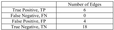
Table 2.0 shows the comparison of edges in YOR263C

sub-network between sub-network constructed by Dejori [14] and with the network constructed in this research. True Positive (TP) is the number of edges that exist in network constructed by Dejori and in the network formed in this research. False Negative (FN) is the number of edges that exist in Dejori [14]’s sub-network, but do not exist in the network in this research. False Positive (FP) is the number edges that exist in this research, but not in the network by Dejori [14]. True Negative (TN) is the number of edges that do not exist in the network by Dejori [14] and in this research.

For YOR263C sub-network, the sensitivity (true positive rate)

is 100%. This means that all the 6 edges that exist in Dejori [14] are also exist in the network formed in this research as well. This shows the program used in this research has successfully predicted and formed all the possible existing edges or

interactions between genes in the network like the one by Dejori [14].

Figure 2.1 YOR263C sub-network constructed in this research

Table 2.0 Comparison of YOR263C sub-networks

Number of Edges

True Positive, TP 6

False Negative, FN 0

False Positive, FP 4

True Negative, TN 18

The specificity (true negative rate) is 82%; whereby there are 4

edges formed in the network in this research do not exist in the network by Dejori [14]. The 4 edges are YNR067C with YOR263C, YOR263C with YJL196C, YOR325W with YGL028C, and YOR325W with YOR263C. This shows that the program used in this research is capable of uncovering more edges or interactions between genes if compared with Dejori [14].

Overall, the gene network constructed through this research

shows that the Bayesian networks implemented in this research not only have successfully predicted all the edges that have been constructed by Dejori [14] in his research, but the Bayesian networks implemented are also capable to discover more new possible edges or interactions between genes. Hence, it can be concluded that the Bayesian networks implemented in this research have optimized performance and they perform better than the Bayesian networks developed in Dejori [14]’s research in predicting interactions between genes.

Figure 2.2 shows the YPL256C sub-network that is

constructed by Dejori [14]. The network consists of 12 nodes and 9 directed edges. However, there is one node does not form any edges with other nodes in the network, that is node YGR108W.

There is one directed edge from YPL256C to YIL066C. This

means that there is a causal dependency between these two genes. Gene YPL256C encodes for G1 – cyclin which involves in regulation of the cell cycle. While gene YIL066C involves in DNA replication, which appears in the S-phase. Therefore, a causal dependence of YIL066C from YPL256C is biologically logical since their functions are correlated.

Gene YDR146C encodes for transcription factor that activates

transcription of genes that expressed at the M/G1 boundary and in the G1 phase of the cell cycle. Gene YDR146C regulates YHR023W, which encodes a protein that plays a non-essential role in cytokinesis, in M phase. An unexpected result is that gene YGR108W doesn’t form any edge with other nodes. However, in

a research by Spellman et al. (1998), it formed edges with other

nodes.

YER124C

YLR286C

YGL028C

YNR067

YOR264

YOR263C YJL196C

(5)

Figure 2.2 YPL256C sub-network constructed by Dejori [14]

Figure 2.3 YPL256C sub-network constructed in this research

Figure 2.3 shows the YPL256C sub-network that is constructed in this research. The network consists of 12 nodes and 18 directed edges. The main difference of the network formed in this research with the network done by Dejori [14] is that the number of edges that are found through this research is 2 times more than the one done by Dejori [14]. Besides that, all the edges in the network developed through this research have at least one directed edge with other nodes. However, the network done by Dejori [14] has failed to find or construct any edge for one node, which is YGR108W. All these proved that the methods implemented in this research is able to predict and form more potential edges between genes in a sub-network.

Table 2.1 Comparison of YPL256C sub-networks

Number of Edges

True Positive, TP 8

False Negative, FN 1

False Positive, FP 9

True Negative, TN 12

Table 2.1 shows the comparison of edges formed within

YPL256C sub-network between the network build by Dejori [14] and the network formed in this research. The sensitivity (true positive rate) for this network is approximately 89%, whereby 8 directed edges that exist in the network by Dejori [14] have been captured by the program in this research as well. However, there is one directed edge that exists in network by Dejori [14], but it doesn’t exist in the network by this research, the edge is between YGL021W and YMR001C.

The specificity (true negative rate) for this sub-network is

around 57%. This research has captured 9 new edges between nodes that were unable to be captured by Dejori [14]. The new edges are from YPL163C to YIL066C, from YLR131C to YMR001C, from YIL140W to YPL163C, from YER001W to YIL066C, from YPL163C to YER001W, from YMR199W to YPL163C, from YDR146C to YGR108W, from YDR146C to YGL021W, and from YLR131C to YHR023W.

One of the new edges is directed from YPL163C to YIL066C. Gene YIL066C is expressed only after DNA damage occurred

YPL163C

YMR199W

YPL256C

YER001W

YIL140W YIL066C

YGR108W

YHR023W YLR131C

(6)

in order to cope with the function of YPL163C. Gene YPL163C is responsible in cell rescue, defence and virulence. Therefore, it is biologically logical for YPL163C regulates the expression of YIL066C. Another newly edge that was discovered in this research is from YLR131C to YMR001C. Gene YLR131C encodes the transcription factor that activates transcription of genes expressed in the G1 phase of the cell cycle. On the other hand, YMR001C encodes a protein that is involved in regulation of DNA replication. Therefore, YLR131C is likely to regulate YMR001C.

Overall, the gene network constructed through this research

shows that the Bayesian networks implemented in this research not only have successfully predicted nearly 90% the edges that have been constructed by Dejori [14] in his research, but the Bayesian networks implemented are also capable to discover more new possible edges or interactions between genes. Hence, it can be concluded that the Bayesian networks implemented in this research have optimized performance and they perform better than the Bayesian networks developed in Dejori [14]’s research in predicting interactions between genes.

3.2.2==Escherichia coli

Basically, the gene networks constructed for Escherichia coli dataset through this research cannot be compared with other networks because currently there are no research have construct gene networks from this data using Bayesian networks. Therefore, six genes are selected randomly from the dataset to construct a gene network and then this network is discussed generally.

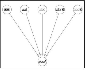
Figure 2.4 Gene network constructed for Escherichia coli

Figure 2.4 shows the gene network constructed for six

randomly chosen genes from Escherichia coli. The gene

network consists of 6 nodes and 5 directed edges. From the network graph, it is clearly shown that the gene node with gene symbol “accA” is co-regulated by all other genes in the graph; they are gene “aas”, gene “aat”, gene “abc”, gene “abrB”, and gene “accB”. This means that the expression level of gene “accA” is dependent on all other genes in the network graph. If one of the genes in the network graph failed to express, then, gene “accA” will not be able to express as well.

Besides that, from the network graph, it is also clearly shown

that the gene expression for gene “aas”, gene “aat”, gene “abc”, gene “abrB”, and gene “accB” are independent. This means that these genes are able to express independently without depending on the expression levels of other genes in the network.

4.0 CONCLUSION

All the methods and algorithms that were implemented in R language in this research have shown that the gene networks constructed through this research have better performance in predicting and discovering interactions or edges between genes. Nearly all the edges that have constructed by Dejori [14] in both YOR263C and YPL256C subnetworks are captured in this research successfully. Besides that, this research has also successfully discovered many new interactions or edges between genes that were failed to be captured in the networks constructed by Dejori [14]. Therefore, it can be concluded the R implementation in this research is a very good and useful tool for scientists to discover and to understand the potential interactions between genes by using Bayesian networks to construct gene regulatory networks.

Acknowledgements

As a token of my appreciation, I would like to thank my supervisor, Dr. Mohd Saberi bin Mohamad for his continuous guidance and advice, also to all my seniors and course mates for their priceless supports and assistances throughout the research process.

References

[1] van Someren, E. P., Wessels, L. F. A., Reinders, M. J. T., and Backer, E. 2001. Robust genetic network modelling by adding noisy data.

Proceedings of the Workshop on Nonlinear Signal and Image Processing (NSIP01) IEEE-EURASIP.

[2] Basso, K., Margolin, A. A., Stolovitzky, G., Klein, U., Dalla-Favera, R., and Califano, A. 2005. Reverse engineering of regulatory networks in human B cells. Nat. Genet. 37: 382–390.

[3] Akutsu, T., Miyano, S., and Kuhara, S. 1999. Identification of genetic networks from small number of gene expression patterns under the Boolean network model. Pacific Symposium on Biocomputing. 4: 17– 28.

[4] Mao, L. and Resat, H. 2004. Probabilistic representation of gene regulatory networks. Bioinformatics. 20(14): 2258–2269.

[5] Bansal, M., Belcastro, V., Impiombato, A. A., and Bernardo, D. 2007. How to infer gene networks from expression profiles. Molecular Systems Biology. 3: 78.

[6] Eisen, M. B., Spellman, P. T., Brown, P. O., and Botstein, D. 1998. Cluster analysis and display of genome-wide expression patterns.Proc. Natl. Acad. Sci. USA. 95: 14863–14868.

[7] Huang, S. 1999. Gene expression profiling, genetic networks, and cellular states: an integrating concept for tumorigenesis and drug discovery. Journal of Molecular Medicine. 77: 469–480.

[8] Friedman, N., Linial, M., Nachman, I., and Pe’er, D. 2000. Using Bayesian networks to analyze expression data. J. Comput. Biol. 7(3): 601–620.

[9] Steele, E., Tucker, A., Hoen, P. A. C., and Schuemie, M. J. 2009. Literature-based priors for gene regulatory networks. Bioinformatics. 25(14): 1768–1774.

[10] Spellman, P.T., Sherlock, G., Zhang, M. Q., Iyer,V. R., Anders, K., Eisen, M. B., Brown, P. O., Botstein, D., and Futcher, B. 1998. Comprehensive identification of cell cycle-regulated genes of the yeast Sacccharomyces cereviciae by microarray hybridization. Molecular Biology of the Cell. 9: 3273–3297.

[11] Kim,H., Golub,G.H., and Park,H. (2005). Missing value estimation for DNA microarray gene expression data: local least squares imputation.

Bioinformatics. 21: 187–198.

[12] Pearl, J. 1988. Probabilistic reasoning in intelligent systems: networks of plausible inference. Morgan Kaufmann.

[13] Marco, S. 2010. Learning Bayesian networks with the bnlearn R package. Journal of Statistical Software. 35(3).

[14] Dejori Mathaus. 2002. Analyzing gene-expression data with Bayesian networks. Graz University of Technology: Master Thesis.