Information Spreading in Dynamic Networks.

(1)

ABSTRACT

KESHAVA NAYAK, ANUJ. Information Spreading in Dynamic Networks. (Under the direction of Dr. Huaiyu Dai).

Today, the interest of network study has spanned multiple disciplines, ranging from technological networks such as the Internet and mobile communication networks to bi-ological networks such as molecular and species interaction networks. The dynamics in-volved in these networks, referring to the changes of either the network state or its under-lying structure, impose challenges to the corresponding studies. In this thesis, information spreading in dynamic networks is studied in the following contexts: opinion maximiza-tion in social networks, dynamic advertising in vehicular ad-hoc networks (VANETs), and rumor spreading in time-varying graphs.

(2)

in synthetic and real-world networks, we demonstrate two key results: 1) the proposed methods perform better than random spreading by a large margin, and 2) even though the smart source (that spreads the desired content) is unfavorably located in the network, it can outperform the contending random sources located at favorable positions.

Second, we address the problem of dynamic advertising in VANETs. We consider a city divided into a grid, where the blocks have different vehicular densities that vary over time. Several advertising companies compete for the blocks to broadcast their advertisements in the network. To solve the problem of block allocation, the repeated auction scheme is adapted for the dynamic setting. We propose an algorithm which is a combination of adaptive linear prediction and nonparametric Bayesian belief update, enabling smart bidding and improving the utilities of the competing advertising companies significantly in the long-run. Through simulations, we show that the proposed algorithm achieves better performance than two baselines approaches.

(3)

(4)

Information Spreading in Dynamic Networks

by

Anuj Keshava Nayak

A thesis submitted to the Graduate Faculty of North Carolina State University

in partial fulfillment of the requirements for the Degree of

Master of Science

Electrical Engineering

Raleigh, North Carolina 2018

APPROVED BY:

Dr. Brian Hughes Dr. Hamid Krim

Dr. Huaiyu Dai

(5)

DEDICATION

(6)

BIOGRAPHY

(7)

ACKNOWLEDGEMENTS

I would like to extend my gratitude towards my advisor Dr. Huaiyu Dai for providing guidance constantly throughout my research. His suggestions were very valuable for my thesis.

I express my gratitude to the rest of my thesis committee: Dr. Brian Hughes and Dr. Hamid Krim for their questions and comments.

(8)

LIST OF TABLES

(12)

LIST OF FIGURES

Figure 1.1 An example of a Bayesian Network. . . 8

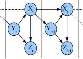
Figure 1.2 An example of a Dynamic Bayesian Network . . . 8

Figure 2.1 Illustration of the system model: Network structure, communica-tion and evolucommunica-tion of opinions in a social network. . . 13

Figure 2.2 Toy Example. . . 19

Figure 2.3 Diminishing returns. . . 20

Figure 2.4 Convergence of expected reward to the optimal value. . . 20

Figure 2.5 DBN representation. . . 24

Figure 2.6 Influence diagram. . . 24

Figure 2.7 N-step look-ahead algorithm. . . 24

Figure 2.8 Timeline for different algorithms. . . 28

Figure 2.9 Effect of centrality and evolution of total opinion for different al-gorithms in PA graph of 103 _nodes. _{. . . 39}

Figure 2.10 Evolution of total opinion and final opinion for different algorithms in PA graph and Facebook ego-network. . . 40

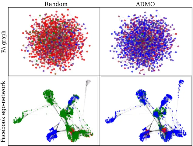
Figure 2.11 Visualization of the evolution of opinions in graphs and the tem-poral evolution of beliefs. . . 41

Figure 3.1 Top level diagram depicting the bidders interacting with the data management unit and the advertisement broadcasting in a VANET. 48 Figure 3.2 Average cumulative utility (top) and percentage increase in average cumulative utility (bottom) under static block densities. . . 59

Figure 3.3 Average instantaneous reward (top) and average instantaneous cost (bottom) under static block densities. . . 60

Figure 3.4 Average cumulative utility (top) and percentage increase in average cumulative utility (bottom) under time-varying block densities. . . . 61

Figure 3.5 Average instantaneous reward (top) and average instantaneous cost (bottom) under time-varying block densities. . . 62

Figure 4.1 eMEG ER graph: Evolution of edges . . . 66

Figure 4.2 Transition rate diagram for the evolution of edges in time-varying NR graph . . . 66

Figure 4.3 Morph-and-Gossip paradigm . . . 69

Figure 4.4 Density and dynamics of graph for different values ofα and β (not to scale) . . . 71

(13)

(14)

Chapter 1 Introduction

Study of dynamic networks can be broadly classified into two categories:

• Dynamics on the networks that refers to the behavioral dynamics or the temporal dynamics of the internal state of the network. Popular examples include the opinion dynamics in social networks, temporal traffic variations in the Internet, and varying loads on electrical grid.

• Dynamics of the networks which deals with the structural dynamics or the topolog-ical variations of the network with time. Examples include ad-hoc communication networks like VANETS (Vehicular Ad-hoc Networks), instant messaging networks, online social networks (like Twitter, Facebook, etc.), and neural dynamics in the human brain.

(15)

spreading in time-varying graphs belongs to the second category, since the underlying network structure varies with time. In the subsequent sections, we provide a brief overview of the aforementioned topics and the background required for the subsequent chapters.

1.1 Smart information spreading for opinion

maxi-mization in networks

1.1.1 Motivation

(16)

peer-to-peer communication. Gossip-based information exchange is a popular method to model peer-to-peer communications among the entities in large-scale distributed systems [40]. Some common applications range from peer-to-peer file sharing systems, consensus formation in networks to distributed signal processing. Gossip algorithms are attractive particularly because of their scalability and robustness. In [17], the idea of social gossip is proposed for spreading recommendations in social networks. There are multiple works on peer-to-peer recommendation systems based on gossip protocols such as PREGO [34] and P2Prec [16].

1.1.2 Related Work

The problem of opinion maximization in social networks is studied in [19] for the first time, where the objective is to find a set of seed nodes whose positive opinion about a desired content maximizes the overall affinity towards it. Some heuristic algorithms are proposed, namely, freeDegree, RWR, etc., and evaluated in large-scale bibliographi-cal datasets. Their approach is similar to the extensively studiedinfluence maximization

(17)

in [8], where the influence spread depends on the distribution of multiple topics. They propose a sample-based algorithm, in which influence spread by every seed node is com-puted faster by avoiding computations that involve users with small influences. In all the aforementioned works, the opinion or influence maximization is regarded as a problem of finding a subset seed nodes. Moreover, in these works information spreading, governed by the underlying model, is passive in nature. Our approach is fundamentally different: we approach the problem of opinion maximization from the angle of smart information spreading.

1.2 Dynamic advertising in VANETs using repeated

auctions

1.2.1 Motivation

Vehicular ad-hoc network is an active research area due to its promising potential in im-proving road safety and transportation efficiency [48]. Most of the research in VANETs has been focused on routing protocols, broadcasting algorithms and security [3, 33]. More-over, there are ample open challenges in the area of VANETs that need to be resolved, ranging from standardization, development and deployment.

An important factor which can boost applications of VANETs is the advent of au-tonomous cars by around 2020. Henceforth, people would be able to perform other tasks, like checking emails, reading news, watch videos, etc., in the vehicles. Also, the mobility and increased connectivity enable several new opportunities such as multimedia stream-ing, and vehicular social networking [45].

(18)

is very high [44]. The advent of autonomous driving and multimedia broadcasting in VANETs provide a great opportunity for commercial companies to capitalize on this segment to advertise their products and services.

In the scenario considered in our work, it is assumed that a city is divided into a grid of blocks with different densities of vehicles varying dynamically over time, and there is a data management unit which handles content dissemination in the network. Several ad-vertising companies compete for accessing the blocks to broadcast their advertisements. The data management unit conducts repeated auctions to rent out the VANET infras-tructure in each block to the advertising companies. The advertising companies act as bidders, who bid repeatedly in successive time-slots for the blocks depending on their valuations.

1.2.2 Related Work

(19)

SUs-SAPs and SAPs-PUs, 1 _{respectively, with a focus on the static network. In [25],} optimal bidding in repeated auctions is discussed for the spectrum access problem, and a distributed learning based bidding algorithm is proposed. The primary emphasis of this paper is on optimal bidding with budget constraints. However, we focus on repeated auctions and judicious bidding with the help of learning and prediction methods in a general dynamic setting.

1.3 Information spreading in time-varying networks

1.3.1 Motivation

“How fast does the information spread” is an interesting question in the context of viral marketing, political campaigning, fake news mitigation, etc. A lot of networks in real world are time-varying in nature with the underlying topology in mobile networks or human activity in online social networks varying in time. This makes the analysis challenging. There are only a few works which propose mathematical models for time-varying networks. One of the first works in this direction is [7], primarily definitional in nature; however, no concrete time-varying network model is proposed. In [50], some widely used static graph models are extended to provide simple and elegant time-varying networks, where the edges evolve as independent Markov processes. This class of time-varying graphs are called edge-Markovian Evolving Graphs (eMEGs). Moreover, there are only a few works that study rumor spreading (gossip) in time-varying graphs as reviewed below. Therefore, the area is challenging and there is significant scope for research.

1_{VCG - Vickrey-Clarke-Groves, SU - Secondary Users, PU - Primary Users, SAP - Secondary Access}

(20)

1.3.2 Related Work

In [12], rumor spreading time is studied for Markovian Erd¨os-R ˙enyi (ER) evolving graphs using Push protocol. In [49], rumor spreading time for random geometric graphs is pro-vided. The concept ofmobile conductance is introduced in [49], which is an extension of

conductance defined for static graphs in [40]. This provides a convenient way to determine rumor spreading time since they are related as [40]:Tsprd() =O(logn+log

−1

Φ ), where>0 and Φ is the conductance. The definition ofmobile conductance provided in [49] holds for general Markovian evolving graphs. Therefore, we adopt this metric to evaluate rumor spreading time for eMEGs.

1.4 Background

1.4.1 Dirichlet Distribution

Dirichlet distribution is a generalization of beta distribution to multi-dimensional case. Since Dirichlet distribution is the conjugate prior of the multinomial distribution, it is commonly used in Bayesian learning.

Definition 1. The Dirichlet distribution [42] is defined as

Dir(α1, ..., α_M) ≜ ∏

M

i=1Γ(αi)

Γ(∑M_i₌₁αi) M

∏

i=1 xαi−1

i , (1.1)

where[x_i]_1≤_i_≤∣Θ∣is the support with∑M_i₌₁xi=1,(∀i∈ {1,2, ..., M})x_i >0, and{α_i, ..., α∣Θ∣}

are the scaling parameters.

(21)

Figure 1.1 An example of a Bayesian Network.

Figure 1.2 An example of a Dynamic Bayesian Network

1.4.2 Dynamic Bayesian Networks

Bayesian network (BN) is a probabilistic graphical model which uses a directed acyclic graph to represent random variables and the conditional dependencies among them. The nodes represent the random variables and the directed edges represent the conditional dependencies. In Figure 1.1, the nodes A, B and C represent the random variables. In this case, the joint distribution is given as

P(A, B, C) =P(A)P(B)P(C∣A, B). (1.2)

Dynamic Bayesian networks are BNs enriched by taking time into account [14]. An exam-ple of DBN is given in Figure 1.2. DBNs are widely used in speech recognition, robotics (e.g., Kalman filter) and data mining applications.

(22)

1.4.3 Network Models

In this section, we briefly introduce some static graph models.

Erdo¨s-Re˙nyi graph[4] denoted as G(n, p), is a random graph of n nodes where the

edges are formed between every pair of nodes with probability p. This model is popular due to its analytical tractability.

Preferential Attachment graph is widely used to model social networks. The preferen-tial attachment mechanism is defined follows: The network is inipreferen-tialized with a complete graph of m ∈_N nodes. Every incoming node i has m edges, each of which are attached

to the existing nodes with probability proportional to their degree. This leads to the so-called “rich gets richer” phenomenon and results in a graph that has heavy-tailed distribution.

Norros-Reittu graph[37] is a random power-law graph, where each node i in the net-work is associated with a weightwi and weights(w_i)_1≤_i_≤_nfollow a power-law distribution.

It is a multi-graph where the number of edges between each pair of nodes is Poisson dis-tributed with mean wiwj

W , whereW = ∑ n

k=1wk. This graph is used over PA graph to study

information spreading because it simplifies analysis.

Note that our focus is on time-varying networks. In chapter 4, we will introduce dynamic versions of the aforementioned models.

1.4.4 Gossip-based Information Spreading

(23)

scalability and robustness. In this thesis, we consider synchronous gossip, where every node ticks according to a global clock. In gossip protocol, each node chooses one of its neighbors uniformly at random. If the node has information, then it pushes the infor-mation to it neighbor, otherwise, it will pull rumor from its neighbor (given that the neighbor has the rumor). If the interaction is between the like nodes, i.e., informed-to-informed or uninformed-to-informed-to-uninformed-to-informed, then no change can be observed in the informed-to-informed status of the nodes. For >0, the -spreading time is defined as

Tsprd() ≜sup

s∈V

inf{t∣P(∣S(t)∣ ≠n∣S(0) =s) ≤}, (1.3)

where n= ∣V∣, V is the set of nodes and S(t) is the set of nodes informed at timet. Conductance: Conductance provides a convenient way to obtain bounds on rumor spreading time in networks. Let P be the transition matrix, where each element Pij

denotes the probability that node i pushes to node j. The conductance for static graphs is defined as[40]

Φ(P) ≜ min

S(t)⊆V ∣S(t)∣≤n/2

⎧ ⎪ ⎪ ⎪ ⎪ ⎪ ⎨ ⎪ ⎪ ⎪ ⎪ ⎪ ⎩ ∑

i∈S(t),j∈S(t) Pij

∣S(t)∣ ⎫ ⎪ ⎪ ⎪ ⎪ ⎪ ⎬ ⎪ ⎪ ⎪ ⎪ ⎪ ⎭ , (1.4)

(24)

Chapter 2 Smart Information Spreading for

Opinion Maximization in Social

Networks

(25)

2.1 System Model

2.1.1 Network Model

Consider an undirected graphG= (V, E), whereV andEare the set of vertices and edges,

respectively. The vertex setV is partitioned into two disjoint subsets V =V_S⊍V_R, where

VS and VR denote the set of source nodes and regular nodes, respectively. The source

nodes in-turn consist of smart sources ˜V and random sources Vr, i.e., VS =V˜ ⊍V_r, that

employ smart and random information spreading processes, respectively. Throughout the chapter, we consider only one smart source node, i.e., ∣V˜∣ = ∣{v˜}∣ = 1, and one or more

random source nodes in the network (∣V_r∣ ≥1). Without loss of generality, it is assumed

that every source node vS ∈V_S injects its own distinct messages into the network at each

time slot. The regular nodes vR ∈ VR facilitate the propagation of information across

the network by forwarding the message to their neighbors. Each regular node vR ∈V_R

has a time-varying feed F(vR)

t of a fixed finite size L. Upon reception of a message, it is

stored in the feed in a FIFO (first-in-first-out) manner. Let M be the set of messages circulated in the network, and let UΘ=Θ⊍θ¯be the set of distinct message classes. The

set Θ can be interpreted as a set of categories of competing products advertised by a company or ideologies in political campaigns, and each message is analogous to a specific advertisement or a particular propaganda, respectively, while class ¯θ includes personal messages. We define the inclination as the mapping I ∶ M →UΘ ∶m ↦ ϑ, which maps

each message to a class. The regular nodes can transmit messages of any class inUΘ, while each source node transmits messages corresponding to a fixed class in Θ. Henceforth, it is assumed that the smart source injects messages of class ˜θ∈Θ into the network. Next,

(26)

I(f1) = θ1

I(f2) = θ1

I(f5) = θ3

Would you like to forward to Bob?

choose w.p. 0.225 forward w.p. 0.5 ignore w.p. 0.5 Alice Dave Eve Bob Ted

μ_t(Alice)_{= (0.5, 0.25, 0.25)} 0.5 0.25 0.25 Alice

α_t(Bob)_{= (2, 2, 2)} Bob

0.5 0.5 0.5 Mike

I(f4) = θ2

0.375 0.375 0.25 α_t+1(Bob)_{= (3, 3, 2)}

Alice Ted Bayesian update Alice's Smartphone Network Model Communication Model

Bayesian Communication Learning Bob's Smartphone FIFO feed Smart source Random source Random source

Θ = {θ₁, θ₂, θ₃} β(Bob)_{, ζ}(Bob)_{= 1} P_sp = 0.1

Smart spreading: Alice Random spreading: Eve, Ted

N_Θ= 4

w.p. 0.1 Transmit

Personal message

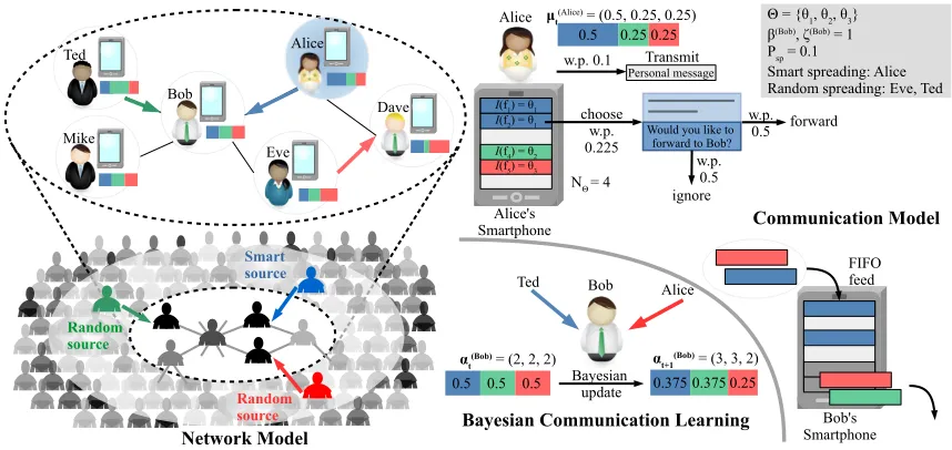
Figure 2.1Illustration of the system model: Network structure, communication and evolution of opinions in a social network.

strength of opinions of a user in social network.

Definition 2. Let{α_θ,t(v)}be the set of belief parameters that represent the affinity of node

v towards class θ at timet∈ {0,1, ..., T},∀v∈V and ∀θ∈Θ. Then, for node v the overall

strength of opinions is defined as ρ(v)

t ≜ ∑θ∈Θα (v)

θ,t, and the opinion of node v about the

class θ is defined as µ(v)

θ,t ≜α

(v)

θ,t/ρ

(v)

t . Consequently, the support of individual opinions is

the simplex [µ(_θ,tv)]_θ_∈Θ∈R∣Θ∣, where∑_θ_∈Θµ

(v)

θ,t =1.

Next, we present the communication model, in which the interaction between the nodes is governed by their current opinions.

2.1.2 Communication Model

(27)

dissemina-tion and political campaigning, the communicadissemina-tion is predominantly push-based since the target individuals are unaware of the impending message. In our model, a regular node exhibits the following characteristics: 1. spontaneously generate and push personal messages (class ¯θ) with probability (w.p.) Psp, or else (w.p. 1-Psp) 2. push (forward) a

messagef of class Θ from its feed w.p.Pf to one of its neighboring nodes. In the latter,

we assume that the messagef is chosen uniformly at random (u.a.r.) from the messages of class Θ in the feed and transmitted w.p. µθ, where θ = I (f). Therefore, P_f = µθ

NΘ,

whereNΘ is the number of messages of class Θ in the feed; the dependency ofPf on the

opinionµθ is a reasonable choice, since users in social networks mostly forward messages

that align with their opinion. We assume that the personal messages are not forwarded. A source generates messages at rate Rm and pushes them to one of its neighbors at

every time step. In our model, we assume that at every node the messages correspond-ing to random sources (class Θ∖θ) are forwarded to one of its neighbors u.a.r., while˜

the messages of the smart source (the messages of class ˜θ) are forwarded using certain mechanism (discussed in subsequent sections). Next, we describe the opinion evolution as a time-varying Dirichlet distribution.

2.1.3 Evolution of Opinions

(28)

is updated based on inclination of the message. Since a node can receive messages from multiple neighbors, we treat the incoming messages corresponding to multiple classes as multinomial observations. Consequently, the posterior belief is in-turn a Dirichlet distri-bution, since it forms a conjugate pair with multinomial distribution.

2.1.3.1 Bayesian Communication Learning

We assume that the nodes have heterogeneous learning behaviors, where certain nodes trust the incoming messages strongly and make a significant update to their belief, while others are stubborn nodes that must be persuaded more to alter their beliefs. Moreover, some nodes have higher retention of social learning than others. For every nodev ∈V_R, the

two aforementioned behaviors are captured using the node specific parameters, ζ(v)

>0

and β(v)

∈]0,1[, respectively. Let n(_θ,tv) be the number of incoming messages of class θ∈Θ

at timet. Nodev updates its belief parameter as per the following rule:

α(v)

θ,t =β

(v)_α(v)

θ,t−1+ζ (v)_n(v)

θ,t. (2.1)

Therefore, the posterior belief is given by

(G(_tv)(θ1)...G(_tv)(θ∣Θ∣))∣n(₁v), ...,n(_tv)

∼Dir(β(v)α₁(v_,t)₋₁+ζ(v)n₁(_,tv), ..., β(v)α(_∣Θ∣v)_,t₋₁+ζ(v)n(_θ,tv)),

(2.2)

where Gt is a random distribution over Θ at time t, and n

(v)

τ = (n(_θ,τv))

θ∈Θ. It can be observed in Eqs. (2.1)-(2.2), that the magnitude of belief parameter (hence the opinion) is proportional to the number of incoming messages of the corresponding class.

(29)

messages are generated by the smart source. For illustration, we zoom-in to observe a sub-network of 6 users at time t. Alice chooses a message f2 from her feed w.p. 1−Psp

NΘ =

0.9 4 = 0.225. which consists of a recommendation to forward the message to Bob. Then, Alice forwards the message to Bob w.p.µ(Alice)

θ1,t =0.5. Note that the forwarding recommendation

is smart since Bob is more influential (clarified later) than her neighbor Dave. On the other hand, Eve selects a message of class θ3 from her feed which consists of a random recommendation to forward the message to Dave. Ted and Mike push message (u.a.r.) of class θ2 and a personal message to Bob, respectively. Also, the FIFO feed and belief parameter update by Bob upon receiving messages from Ted, Alice and Mike is depicted in the Figure 2.1. Note that the personal message from Mike does not modify the opinion of Bob. The goal of the smart source is to generate smart forwarding recommendations for those nodes that have chosen message of class ˜θ (in this case Alice) from their respective feeds so that the overall opinion towards the smart source is maximized. In the next section, we provide a mathematical treatment of the opinion maximization problem.

2.2 Problem Formulation

In this section, first a formal definition of the opinion maximization problem is provided, which is followed by the discussion of a toy example where we solve the problem in closed form. Then, in order to extend the ideas for general case (arbitrary connected networks and considering the factor of time), we present dynamic Bayesian network and influence diagrams, which will be used subsequently to develop algorithms to achieve opinion maximization. To begin, we define theaction taken by the nodes in the network.

(30)

Then the action of node v is a(v)

t =w.

We denote the joint action asat= (a(_tv))

v∈V˜t

, where the set ˜V_tdenotes the set of nodes

that have chosen message of class ˜θfrom their feeds at time t. The objective of the smart source is to maximize the opinion of individuals in the social network towards class ˜θ. The formal definition of opinion maximization is given as follows:

Definition 4. Let(a_t)_0≤_t≤T−1 be the sequence of joint actions andα0 = [α (v)

θ,0]v∈V

θ∈Θ be belief parameters at time t=0. The objective of the smart source is to maximize the expected

total opinion of class ˜θ at time T, which is given as

maximize (at)₀_≤_t_≤_T₋₁ E

{ ∑

v∈V µ(v)

˜

θ,T ∣ (at)0≤t≤T−1,α0}. (2.3)

In Appendix A.1, the opinion maximization problem is analyzed for a simplified ver-sion of the communication model described in 2.1.2. In view of Eq. (A.4) in Appendix A.1, we define the reward as follows:

Definition 5. The reward obtained by node v when it pushes a message of class ˜θ to w∈N(v) is defined as:r(v)(w) ≜

µ(_˜w)

θ,t (1−µ

(w)

˜

θ,t)

µ(_˜w)

θ,t+α

(w)

˜

θ,tβ

(w)/ζ(w) .

Observation 1. In Definition 5, the reward indicates the change in opinion of nodewabout class ˜θ. Moreover, the best myopic action is to push the message to a node with weakly neutral opinion. For instance, let β, ζ = 1 and α_θ,₀ =1, ∀θ ∈Θ, then the instantaneous

reward rt≈

µ˜_θ,t(1−µ˜_θ,t)

(31)

2.2.1 A Toy Example of Opinion Maximization

In this section, we present a toy model, where the problem is solved in closed form. The purpose of the toy model is to obtain some insights, which are later used to develop algorithms for large-scale networks. The toy model consists of 4 nodes with 2 transmitters (x and y) which can push message of class θ1 ∈ Θ, to one of 2 receivers (c and d),

independently. The actions of the nodes x and y are denoted as a(x)

∈ {c, d} and a(y)∈ {c, d}, respectively1. Moreover, the opinions of nodesxand yabout classθ1 is considered

to be µ(x)

θ1 = µ

(y)

θ1 = 1; therefore the action a

(i)

=j is equivalent to saying node i pushes

message to node j, ∀i∈ {x, y} and ∀j ∈ {c, d}. Both the receivers are Bayesian learning

agents with the opinions about the two message classes (θ1 and θ2) denoted as µ(i)

θ1 and

µ(i)

θ2 (i ∈ {c, d}), respectively. Both the nodes x and y are oblivious to the actions of

the other. If only node x pushes to node c, then from Eq. (A.4) the change in opinion is given as: µ(c)

θ1 µ

(c)

θ1 (µ

(c)

θ1 +α

(c)

θ1 β

(c)

/ζ(c))−1 =

α(_θc) 2ζ

(c)

(β(c)ρ(c)+ζ(c))ρ(c), which we call the individual reward rc. Similarly, the individual reward rd=

α(_θd) 2ζ

(d)

(β(d)ρ(d)+ζ(d))ρ(d). The nodes x and y have the knowledge of opinions of the nodes cand d. Consequently, they know the individual rewardsrc and rd. We call the joint reward as the total change in opinion when both the

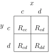
nodes x and y transmit to nodes c or d. The joint rewards for all the combinations of joint actions (ofx and y) are given in Table 2.1, and are not known tox and y a priori. The joint rewards are given by

Rcd= ∑

j∈{c,d}

α(j)

θ2 ζ

(j)

(β(j)ρ(j)+ζ(j))ρ(j),

(2.4)

(32)

and

Rii=

2α(i)

θ2 ζ

(i)

(β(i)ρ(i)₊2ζ(i)₎ρ(i), ∀i∈ {c, d}. (2.5) The objective is to determine the strategy, i.e., the best choice of actions, such that the total opinion (µ(c)

θ1 +µ

(d)

θ2 ) is maximized. In this scenario, we state the following

proposi-tion that provides the condiproposi-tion where pure strategy (rule that maps individual rewards to the actions) does not yield the maximum reward, and also determine the mixed strat-egy (probability distribution over actions/pure strategies) that results in the maximum reward.

y

x

c d

c Rcc Rcd

d Rcd Rdd

Table 2.1 Reward Table.

x

y

c

d

c

d

Rcc Rdd

R

x

y

cd

Figure 2.2 Toy Example.

Proposition 1. In the aforementioned toy example, if

1 1+η(c) <

rd

rc

<min{1,(

1+η(c)

1+2η(c)) (

1+2η(d)

1+η(d) )}, (2.6)

then the maximum reward is given by the mixed strategy, π = (p,p¯ = 1−p), where

p=P(a(x)=c) =P(a(y)=c) = (1+_RRcd−Rcc

cd+Rdd)

−1

and η(i)

= ζ

(i)

β(i)ρ(i), ∀i∈ {c, d}.

(33)

Informally speaking, the proposition states that in the toy example if the nodescand dhave similar beliefs, then the better strategy for nodesxandyis to take distinct actions (non-diagonal elements in Table 2.1). This phenomenon is illustrated using a numerical example in Figure 2.3. It can be observed that the reward ∆µθ1 exhibits diminishing

returns with respect to the number of incoming messages nθ1, which underscores the fact

that taking distinct actions yields higher reward Rcd =r_c+r_d. In large-scale social

net-works, many nodes have common neighbors (e.g., mutual friends). Taking selfish actions implies that multiple nodes try to persuade one of their common neighbors to change its opinion. This could lead to lower joint rewards and also restrict information spreading. On the other hand, using mixed strategy helps in better information spreading and yields better joint rewards.

= 0.167 = 0.1

= 0.083

Figure 2.3 Diminishing returns.

5 10 15 20

Number of samples (

N

S

)

0.17 0.175 0.18 0.185

E

π

{

r

}

Eπ,N_S(r(a∗))

Max. joint reward

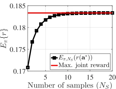
Figure 2.4 Convergence of expected reward

to the optimal value.

Definition 6. Let h(1) and h(2) be the rewards obtained by taking two distinct actions

(34)

soft-max) is defined as

Ξ(h, i,T ) ≜exp(h(i)/T )/ (Σ2_j₌₁exp(h(j)/T )), (2.7)

where T >0 is the temperature parameter.

Remark 1. Given a mixed strategy π= (p,p¯), if p>p¯and h(1) >h(2) >0, then ∃ T >0

such that (p,p¯) = (Ξ(h,1,T ),Ξ(h,2,T )) (the proof is straightforward). This implies

that in the aforementioned toy example with two actions, the mixed strategy can be obtained exactly using the individual rewards and Boltzmann distribution by tuning T

appropriately. However, if the number of actions is greater than 2, then it can be easily verified that the mixed strategy can only be approximately obtained.

Remark 2. Sampling Improves Expected Reward: Consider a central controller which is capable of controlling joint actions a= (a(x), a(y)) and observe the joint rewards. It can

try multiple joint actions offline and determine the best joint action (that gives the maximum joint reward) from history, following which it is executed. In particular, the central controller samples joint actions from the distributionπ=π×π,N_S times (denoted

as a NS

∼ π). The best joint action is given by: a∗ = argmax

aNS∼πRa

. Let p′

=1−2pp¯and

p′′_{= (}₁₋p2_/(p2₊p_¯2₎₎_{. The expected joint reward is given by}

Eπ(R_a∗) = (1−p′Ns)R_cd +p′Ns((1−p′′)NsR_cc+p′′NsR_dd). (2.8)

As shown in Figure 2.4, we can observe that lim

Ns→∞Eπ

(R_a∗) =R_cd, which is the maximum

joint reward in Table 2.1.

(35)

can be used to obtain the mixed strategy (Remark 1), and 3. sampling improves the expected reward (Remark 2). In the toy model, we considered a single snapshot of a small network. We extend the ideas of the toy model to larger networks and also take the factor of time into account. Therefore, we begin with the DBN representation of opinion dynamics as follows.

2.2.2 Representation of Opinion Evolution in the Network as a

Dynamic Bayesian Network

Dynamic Bayesian networks (DBNs) are probabilistic graphical models where the nodes stand for random variables, and their conditional dependencies and temporal relation-ships are represented through a directed acyclic graph [28]. Two time-slices are required to fully represent the dynamics: one for indicating conditional relationship between ran-dom variables, and the other for depicting the causal dependence. This representation helps in developing approximate iterative algorithms for sequential decision problems.

LetX(v)

θ,t be a random variable that represents the belief parameterα

(v)

θ,t, wherev ∈V

and θ ∈ Θ. We construct a random matrix X_t = [X_θ,t(v)]_v∈V

θ∈Θ, which captures the belief parameters of the entire network at time t. Similarly, let Ωt = [Ω(_tv)]_v∈V be a random vector, where each element Ω(v)

t is a random variable representing the inclination of

messagem(v)

t chosen by node v from its feed at time t. Let Ft= [F_j,t(v)] v∈V 1≤j≤L

be a random matrix where each element is a random variable that represents the jth _{message in the} feed of node v at time t. Finally, let At = [A_t(v)]_v∈V be a random vector, where A

(v)

t

(36)

whether the message should be forwarded or not based on their current opinions. Then, based on the actions of the nodes and the class of the chosen messages, the beliefs of the recipient nodes are updated. The newly received messages update the feeds by occupying the top positions, while pushing out the older messages. We represent these dynamics using a DBN as shown in Figure 2.5.

2.2.3 From DBN to Influence Diagram

In decision theory, some variables of a DBN are converted to decision variables and utility variables, and the whole model is alternatively called an influence diagram. In our model, the influence diagram (Figure 2.6) is constructed from DBN as follows. We assume that Ft cannot be observed; hence, the uncertainty nodeFtof the DBN and all the associated

edges (both incoming and outgoing) are removed from the influence diagram. Even though the removal is not optimal, it makes our analysis tractable. The uncertainty node At is

converted to a decision node at2. Before determining action at, the random variables Xt

and Ωtare observed. Hence, informational arcs are connected from the observable nodes

to the decision nodeat. The goal of the problem is to determine the optimal sequence of

(37)

X_t Ω t F_t A_t X_t+1 Ω_t+1 F_t+1

Figure 2.5 DBN

rep-resentation.

X

_t

Ω

_t

X

_t+1

Uncertainty Node Decision Node

A

_t Utility Node

A

_t+1

Ω

_t+1

X

_t+1

A

_t+1

Ω

_t+1

X

_T-1

A

_T-1

Ω

_T-1

1

T

_E[g(X

T

)]

X

_t+1

...

Figure 2.6 Influence diagram.

x_t;0 ω_t;0 X_t-2 Ω_t-2 F_t-2 A_t-2 X_t-1 Ω_t-1 F_t-1 A_t-1 Ω_t+N F_t+N A_t+N X_t+N+1 Ω_t+N+1 F_t+N+1 A_t+N+1 ... ... ...

1T_g(α

t;N)

a_t;0,k

π_t;0 ~

α_t;1 ω_t;1 π_t;1 ω_t;N-1 α_t;N-1 π_t;N-1

Known Random Node Deterministic Node

^

^ ^

^

Figure 2.7 N-step look-ahead algorithm.

2.3 Centralized Algorithms

In this section, starting from the optimization problem in Definition 4, we use the influ-ence diagram and ideas from the toy model (Section 2.2.1) to construct a framework, using which we develop centralized iterative algorithms. The central controller possesses∀v ∈V

and∀θ∈Θ the knowledge of the opinionµ(_θ,tv), the overall strengthρ_t(v)= ∑_θα_θ,t(v), the

prob-2_{Henceforth, unless stated otherwise, the values of random variables are indicated by lower case bold}

(38)

ability of spontaneous transmission Psp, the global topology of the network G, and the

locations of all the source nodes. Let g ∶α = [α(_θv)]_v∈V

θ∈Θ

→µ_θ˜ = [α(_˜v)

θ / ∑_θ_∈Θα

(v)

θ ]v∈V be the function that maps belief parameters to the opinions corresponding to class ˜θ. Now, the objective function in Definition (4) is alternatively given as:1TE_[_g₍_X

T) ∣ (a_t)_0≤_t

≤T−1,α0]. From the influence diagram, it can be observed that given Xt, the action at does not

de-pend on past observations. Moreover, Xt is observed at every time step before action at

is decided, which decreases the uncertainty in total opinion at time T. Hence, instead of determining the sequence of actions (a_t)_0≤_t_≤_T₋₁ upfront at time t = 0, the action a_t

that provides the maximum total opinion at time T can be determined at every time t. Therefore, Eq. (2.3) is modified to the following decision problem:

a∗

t =argmax

at

π∗

t ∣ (π

∗

τ)t≤τ≤T−1=argmax (πτ)t≤τ≤T−1

1T_E

ψ{g(X_T) ∣α_t}, (2.9)

where πτ is the probability distribution over joint actions at time τ with πτ(A_τ) =

P(A_τ ∣ Ω_τ, X_τ), a_t∗ is an optimal action at time t, and ψ = f(X_T ∣ α_t) is obtained by

marginalization as follows:

ψ= _∫

Xt+1∶T−1

∑

Ωt∶T−1 At∶T−1

T−1

∏

τ=t

f(X_τ₊₁ ∣X_τ,Ω_τ, A_τ)P(Ω_τ ∣X_τ)π_τ(A_τ). (2.10)

(39)

2.3.1 A Framework for Centralized Algorithms

The basic idea of the framework is to approximate ψ to conveniently compute the objec-tive function 1T

Eψ{g(X_T ∣α_t)}. To be precise, we approximate ψ by making the

condi-tional distributions given in Eq. (2.10) degenerate. This enables us to iteratively compute the objective function. In this regard, three approximations are provided, whose inherent assumptions are explained in 2.3.2.

Approximation 1: Obtaining the mixed strategy profile πτ is computationally

de-manding. Hence, we assume that the distribution of actions taken by the nodes are independent, resulting in the constraint (approximation)

πτ(Aτ) ≈ ∏v∈Vπτ(A

(v)

τ ), (2.11)

whereπτ(A(_τv)) =P_τ(A(_τv)∣Ω_τ, X_τ)is the mixed strategy of nodev. Given this

approxima-tion, we assume that if Ωτ andXτ are observed, then we can obtain the joint distribution πτ.

Due to aforementioned approximations, the actiona∗

t in Eq. (2.9) is no more optimal.

Therefore, using Remark 2, we sample at from πt, and use (πτ)t+1≤τ≤T−1 to approxi-mately compute the objective function. Moreover, for tractability the objective function is modified to 1T_g₍

Eψ{X_T ∣α_t,a_t}), which results in the following decision problem:

a∗

t =argmax

atNS∼πt

1T_g

(_E_ψ{X_T ∣α_t,a_t}). (2.12)

Approximation 2: Given the belief parameters Xτ, we assume that the maximum a

posteriori (MAP) estimate ˆωτ = argmax_ω_∈ΘP(Ω_τ = ω ∣ X_τ) can be obtained. Then we

(40)

ˆ

ωτ. Also, note that probability of spontaneous transmissionPsp can be interpreted as the

probability of choosing message of class ¯θ. Moreover, every node in the network chooses message from its feed independently. Therefore, the conditional distribution of choosing message of any class in UΘ is approximated as

P(Ω_τ ∣X_τ) ≈ ∏

v∈V

(1−P_sp)δ(Ωτ(v)−ωˆτ(v)) +P_spδ(Ω(_τv)−θ¯).

(2.13)

Approximation 3: We assume that if ˆατ, ˆωτ and πτ are known, then the mean

be-lief parameters ˆατ+1 = _E{X_τ₊₁ ∣ α_t,a_t} can be computed. Given this assumption, we

approximate the conditional probability density over Xτ+1 to be degenerate:

f(X_τ₊₁ ∣α_t,a_t) ≈δ(X_τ₊₁−αˆ_τ₊₁). (2.14)

It can be noticed that if Xt=α_t is observed, then using the aforementioned

approxi-mations and the influence diagram, the expected belief parameters ˆαT =E_ψ{X_T ∣α_t,a_t}

can be determined in an iterative manner. Next, we develop centralized algorithms using the framework described so far.

2.3.2 CAMO Algorithm

We develop a Centralized Algorithm for Opinion Maximization (CAMO), where we clar-ify the underlying assumptions mentioned in 2.3.1 by providing some heuristics. First, note that at time t computing the objective function 1T_g₍E

ψ{X_T ∣α_t,a_t}) =1Tg(αˆ_T)

involves T −t steps of computations. This gives rise to two issues: 1) LargeT −t results

(41)

com-...

Push Run algorithm

...

Run algorithm Push

←

τ k → N

K

Algo. Parameters

CAMO N>0 K=1 N_S>0 ACMO N>0 K = K΄ N_S>0

DAMO N=1 K=1 N_S=1

ADMO N=1 K=N_Q N_S=1

N_Ssamples

t t+1

t-1

K΄= max(N-τ, N_Q)

Figure 2.8Timeline for different algorithms.

plexity. To address these, we determine the action a∗

t such that the objective function

is maximized for time t+N instead of that at time T, where N < T is the look-ahead

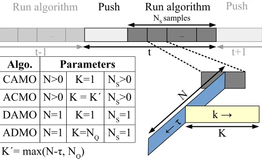
window size. To achieve this, the state of the network is observed at time t, followed by a centralized offline N-step look-ahead procedure. In this regard, we call t as the online time during which the users in the network communicate, the iterations of the algorithm are indexed by τ (offline time) and t;τ indicates the composite time. The timelines for different algorithms are depicted in Figure 2.8. To be precise, given the state of the net-work at time t, the action at;0 must be determined such that the mean total opinion at time t;N is maximized. Note that the mean total opinion att;N is the prediction of the actual future mean total opinion at time t+N. Our algorithm consists of the following

three stages3_:

1. Sampling joint actions at.

2. Computing the objective function 1T_g₍_α_ˆ

T)by probabilistic diffusion.

(42)

3. Repeating the previous two steps NS times, and then choosing sub-optimal joint

action a∗

t.

Next, the aforementioned steps are discussed in detail and the assumptions made in 2.3.1 are addressed.

2.3.2.1 Sampling Joint Actions

1.a) Obtaining ωˆτ: Now, we address the assumption associated with Approximation 2.

Computing the exact ˆωτ = [ωˆ_τ(v)]_v∈V is tedious since the size of the sample space grows exponentially (∣UΘ∣∣V∣) with the network size. Therefore, we assume that every node

pushes a message of the class corresponding to its maximum opinion at time τ. Hence, the MAP estimate ˆω(v)

τ is obtained approximately∀v∈V and ∀τ ∈ [1, N−1]as

ˆ ω(v)

τ ≈θ∈Θ∣αˆ(_θ,τv)≥αˆ(_θv_′_,τ),Θ∋ ∀θ′≠θ. (2.15)

However, at timeτ=0, we assume that central controller has the instantaneous knowledge

of ω0.

1.b) Obtaining πτ:

(43)

˜

θ (similar to that in the toy model). Therefore, the mixed strategy of node v is given by

πτ(A(τv)=w) = ⎧ ⎪ ⎪ ⎪ ⎪ ⎪ ⎨ ⎪ ⎪ ⎪ ⎪ ⎪ ⎩

Ξ(r_τ(v), w,T ), if ω_τ(v)∗=θ,˜

1

∣N (v)∣, if ω (v)∗

τ ≠θ,˜

(2.16)

wherer(v)

τ = (r(_τv)(x))_x_∈_N₍_v₎. Then, the probability over joint actionsπ_τ can be computed

using Eq. (2.11). As mentioned in Remark 2, the joint actiona0 is sampled fromπ0. Then, to compute the objective function1T_g₍_α_ˆ

T), the central controller performs probabilistic

diffusion, which is described as follows.

Algorithm 1: Wrapper Function.

1 Initialize feeds:

2 F_t(v)= (f_i)_1≤_i≤L, ∀v∈V, where I (fi) ∈Θ, and¯ ∀i∈ {1, ..., L}

3 for eacht∈ {1,2, .., T} do

4 Report {α_θ,t(v)}_1≤_θ_≤Θ and ω_t(v) to the central controller, ∀v∈V (For CAMO and

ACMO only).

5 Run learning algorithm: CAMO/DAMO/ADMO/ACMO. 6 Execute action a∗_t_;0.

7 Update belief using Eq. (2.2). 8 Update Feed.

9 end

2.3.2.2 Probabilistic Diffusion

Given α0 and a0, computing ˆαN iteratively is termed as probabilistic diffusion, since

(44)

Algorithm 2: CAMO and ACMO Algorithms.

1 for k∈ {1,2, ..., N_S} do

2 Compute π_t_;0 using Eq. (2.19). 3 Sample a_t_;0_,n fromπ_t_;0 (a_t_;0_,n∼π_t_;0). 4 Initialization:

5 αˆ_t_;0∶=α_t, χmax_t_;_N ∶=0, and compute ˆω_t_;0 using Eq. (2.15). 6 for eachτ ∈ {1,2, ..., N} do

7 Compute ˆω_t_;_τ using Eq. (2.15). 8 Compute ˆα_t_;_τ using Eq. (2.17).

9 CAMO:

10 Compute π_t_;_τ using Eq. (2.16).

11 ACMO:

12 Run ADMO to get π_t_;_τ = (Ξ(Q(_t_;u_τ)_;_K, v,T ))_u_∈_V_∖_V

r

v∈N (u) .

13 end

14 Compute χ_t,N =1Tg(αˆ_t_;_N). 15 if χ_t_;_N >χmax_t_;_N then

16 a∗_t_;0∶=a_t_;0_,n. 17 χmax_t_;_N ∶=χ_t_;_N.

18 end

19 end

the assumption associated with Approximation 3, by deriving the expression for ˆατ+1 as follows.

Computing αˆτ+1:

ˆ

ατ+1=E{Xτ+1∣α0,a0} =E{βXτ+∆Xτ ∣α0,a0}

=β○αˆ_τ + [_E{∆X_θ,τ(v)∣α0,a₀}]v∈V

θ∈Θ,

(45)

where4 _β_{= [}_β(v)

]_v_∈_V, and

E{∆X_θ,τ(v)∣α0,a₀} =ζ(v) ∑

u∈N(v) µ(u)

θ,τπτ(A

(u)

τ =v)(1−P_sp)δ(θ−ωˆ(_τv)).

(2.18)

The derivation of Eq. (2.18) is given in Appendix A.3. To determine αˆτ+1 for τ >0, π_τ

is computed as given in Eq. (2.16). However, to compute ˆα1 the conditional probability π0 is modified as

π0(A(₀u)=v) = ⎧ ⎪ ⎪ ⎪ ⎪ ⎪ ⎨ ⎪ ⎪ ⎪ ⎪ ⎪ ⎩

δ(v−a(₀u)), if θ=θ,˜

1

∣N (u)∣, if θ≠ ˜ θ.

(2.19)

In other words, a nodeuwhich has chosen message of class ˜θfrom its feed, pushes message to nodea(u)

0 , whereas a node that has chosen a message corresponding to a random source selects one of their neighbors u.a.r.

2.3.2.3 Choosing Sub-optimal Action a∗ 0

Let[a₀_,n]_1≤_n≤NS be the actions sampled fromπ0and[αˆN,n]1≤k≤NS be the belief parameters

at timeτ =N. Then the sub-optimal action a∗₀ is chosen as: a∗₀ =argmax a0,n

1T_g

(αˆ_N,n).

2.3.3 ACMO Algorithm

Augmented Centralized algorithm for Opinion Maximization (ACMO) is an improved variant of the CAMO algorithm which is made to piggy-back on ADMO (described in 2.4.3). The main limitation of CAMO algorithm that the individual rewards are computed

(46)

in a myopic manner. To alleviate this problem, at each offline time τ, Q-learning is used to look-ahead in time to compute the individual rewards, and hence obtain better mixed strategies. More precisely, Ξ(r_τ(v), w,T )in Eq. (2.16) is replaced by Ξ(Q(_τv_;_K), w,T ), where

K =max(N −τ, N_Q), and obtaining Q(_τv_;_K) is described in 2.4.3. Note that the composite

time consists of an additional offline timek(depicted in Figure 2.8) to capture Q-learning iterations. Algorithm 1 is the wrapper function, which is a general pseudo-code common for all algorithms. The CAMO and ACMO algorithms are given in Algorithm 2.

2.4 Decentralized Algorithms

In this section, two different variants of decentralized algorithms are presented: 1. Decen-tralized Algorithm for Opinion Maximization (DAMO), and 2. Augmented DecenDecen-tralized algorithm for Opinion Maximization (ADMO).

2.4.1 DAMO Algorithm

DAMO is a special case of CAMO algorithm obtained by usingNS =1 and the window size

N =1. Note that in centralized algorithms, a central controller is required for probabilistic

diffusion and to store joint action-future reward pairs obtained by repeated sampling of joint actions. SettingNS=1 implies that the every node samples the action independently

from its mixed strategy only once, and N = 1 implies that there is no probabilistic

diffusion. This makes the algorithm decentralized. Hence, the action taken at time t is simply,a∗

t ∼πt. The algorithm admits a simple two-step procedure given in Algorithm 3.

(47)

Algorithm 3: DAMO Algorithm.

1 Compute Ξ(r(_tu), v,T ), ∀u∈V ∖V_r. 2 DAMO: Sample a(_tu)∼ (Ξ(r(_tu), v,T ))

v∈N (u)∖u

, ∀u∈V ∖V_r.

2.4.2 Background on Q-Learning

Q-learning is a model-free reinforcement learning algorithm. For any Markov Decision Process, Q-learning can be used to find the optimal policy, which is obtained by learning the so-called action-value function Q(s, a), where a is the action taken when the system

is in state s. In particular, Q(., .) is the expected discounted reward of taking action a

in state s and continuing optimally thereafter [46]. When an agent is in state st, the

probability of taking action at is given by: P(s_t, a_t) = Ξ(Q(s_t), a_t,T ), where T is the

temperature parameter andQ(s_t) = (Q(s_t, a′))_a′. Ifrt(s_t, a_t)is the instantaneous reward

obtained at timet by taking action at when the system is in state st, then the

Bellman-equation to update action-values is given by

Qt+1(st, at) ∶=¯λQt(st, at) +λ[rt(st, at) +γmax a′ Qt

(s_t, a′)], (2.20)

where ¯λ=1−λ and γ∈ [0,1] is the discount factor.

2.4.3 ADMO Algorithm

(48)

pushes the message to w1 myopically. However, despite the immediate reward (change in opinion) being lower, it would be wiser to persuadew2 because it is more influential, and hence would yield higher reward after a few time steps. In the ADMO algorithm, each node selfishly looks ahead in time by exploring beyond neighbors over multiple hops for better rewards, based on which better strategies are determined.

We develop the ADMO algorithm based on the idea presented for the simplified model in Appendix A.1, where a single message circulates in the network and the environment is static. However, in contrast to the simplified model, we observe three differences about opinion dynamics in the actual model described in 2.1.2. 1. There are multiple messages circulating in the network. Hence, every node experiences a dynamic environment due to the change in opinions caused by transmissions of other nodes. 2. Initially a few nodes would be transmitting messages of class Θ. Hence, the opinions of many nodes remains unchanged. Therefore, the environment can be considered to be slowly varying during ini-tial time steps. 3. On the other hand, as time progresses, more number of nodes would be transmitting messages of class class Θ rendering the environment more dynamic. Con-sidering the aforementioned observations, we introduce a time varying discount factor γt = γ′γ′′t, where γ′, γ′′ ∈ [0,1], to weigh down the future rewards. Note that the

dis-count factor decays with time t to account for the environment becoming increasingly dynamic with time. In this algorithm, each node uses the sum of discounted future re-wards (s.o.d.f.r.) as individual rere-wards to determine its mixed strategy independently. The state of the network is observed at time t and s.o.d.f.r. is computed iteratively. We denote the iteration number (learning time) as k and the composite time as t;k.

(49)

as (omitting the t in the composite time t;k without loss of generality)

max (a(_kuk))

0≤k≤T−1−t

T−1−t

∑

k=0 γk

tr

(uk)

k (a

(uk)

k ), (2.21)

where u0 = v. We assume that every node in the network independently attempts to

maximize its sum of future discounted rewards over a finite time horizonT−1−t. In this

respect, the sum of future discounted rewards of nodev when a(v)

0 =x is given by

Q(v)

T−1−t(x) =r

(v)

0 (x) + max (a(uk)

k )

1≤k≤T−1−t

T−1−t

∑

k=1 γk

tr uk

k (a

(uk)

k ), (2.22)

where r(u)

0 (v) is the reward obtained upon pushing message to nodev at time k=0. We generalize Eq. (2.22) for 0≤l≤T −1−t as

Q(v)

l+1(x) =r (v)

0 (x) +γtQ

(x)

lmax(v), (2.23)

where Q(x)

lmax(v) = _wmax

∈N (x)∖v Q(x)

l (w). Node v is excluded from the action set of node x

to avoid back-and-forth influence between a pair of nodes. By comparing Eq. (2.23) with Eq. (2.20), it can be observed that each node employs stateless Q-learning. In this algorithm, each node determines the individual rewards (s.o.f.d.r.) by exchanging the action-values between the nodes. For instance, in Eq. (2.23) node x shares Q(x)

lmax(v)

with node v, which consequently updates its action-value Q(v)

l+1(x). Also, to alleviate the computational complexity, the action-values are updated only for NQ time steps. The

(50)

Algorithm 4: ADMO Algorithm.

1 Initialization:Q(u)(v) ∶=0,∀u∈V ∖V_r , and ∀v ∈ N (u).

2 k∶=0.

3 while k<N_Q do 4

Q(u)

t;k+1(v) ∶=r (u)

t;0(v) +γ

k tQ

(v)

t;kmax,∀u∈V ∖Vr, and ∀v∈ N (u) ∖u.

5 end

6 Compute Ξ(Q(_t_;u_N)

Q, v,T ), ∀u∈V ∖Vr.

7 Sample a(_tu)∼ (Ξ(Q(_t_;u_N)

Q, v,T ))_v_{∈N (}_u₎, ∀u∈V ∖Vr.

2.5 Complexity Analysis

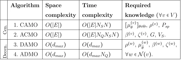
The required knowledge as well as the space and time complexities of different variants of centralized and decentralized algorithms are listed in Table 2.2. In the decentralized algorithms, each node must know the opinions, the overall strength of the opinions and the social learning abilities of only the neighboring nodes. For a given information spreading process (equivalently the source node), the opinion of the neighbors corresponding to only its class must be known. On the other hand, the centralized algorithm requires that the opinions pertaining to all the message classes be known. Moreover, centralized algorithm requires the knowledge of the topology of the graphG, and the locations of all the source nodes VS. Therefore, the centralized algorithms bear a significant overhead compared

to the decentralized variants. In the centralized algorithms, the space complexity is dominated by the storage of action-values of all the nodes, where each regular node v has ∣N(v)∣ action-values resulting in 2∣E∣ action-values for the entire network. This

leads to the space complexity of O(∣E∣). On the other hand, the space complexity of

(51)

Table 2.2 Complexity and required knowledge of the algorithms.

Algorithm Space Time Required

complexity complexity knowledge (∀v ∈V)

Cen.

1. CAMO O(∣E∣) O(∣E∣N_SN) [µ_θ(v)]_θ_∈Θ, ρ(v),P_sp

2. ACMO O(∣E∣) O(∣E∣N_QN_SN) β(v),ζ(v), G,V_S.

Decen.

3. DAMO O(d_max) O(d_max) ρ(w),µ(_˜w)

θ , β

(w)_, ζ(w)_, 4. ADMO O(d_max) O(d_maxN_Q) ∀w∈ N (v).

results in the space complexity of O(d_max), where d_max is the maximum degree in the

network.

The time complexity of the ACMO algorithm is dominated by the probabilistic diffu-sion and repeated Q-learning. Both probabilistic diffudiffu-sion and one-step Q-learning involve about ∣E∣ operations for every offline time τ. Considering N-step look ahead (window of

sizeN),NQ repetitions of Q-learning andNS samples, the number of operations per unit

time (t) of the centralized algorithm is O(∣E∣N_QN_SN). Since the CAMO algorithm is

similar to the ACMO algorithm without Q-learning, its time complexity is O(∣E∣N_SN).

The decentralized algorithms have much lower time complexity. In ADMO algorithm, each node v ∈V performs repeated Q-learning independently, which involves ∣N (v)∣N_Q

operations per unit time resulting in the worst-case time complexity ofO(d_maxN_Q). Since,

the DAMO algorithm does not involve Q-learning, its time complexity is O(d_max).

2.6 Simulation Results

(52)

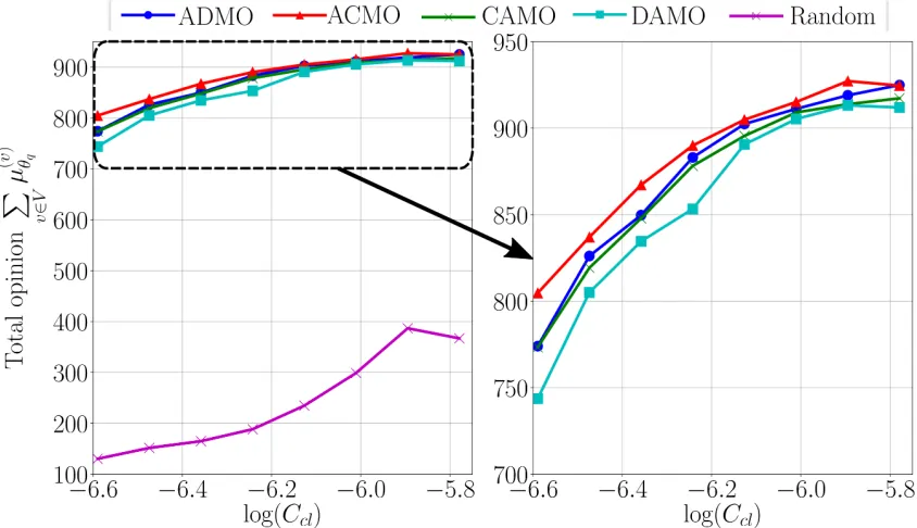
(a)Final total opinion of the population versus the centrality (Ccl) of the smart source for

differ-ent algorithms.

0 20 40 60 80 100

Time (t) 100 200 300 400 500 600 700 800 T ot al op in io n

P v∈

V µ ( v ) θq ACMO ADMO CAMO DAMO Random

0 20 40 60 80 100

P v∈

V µ ( v ) θ θq θ1 θ2

(b) Evolution of total opinion with time: for different algorithms (left), and for 3 different classes when ADMO is used (right).

(53)

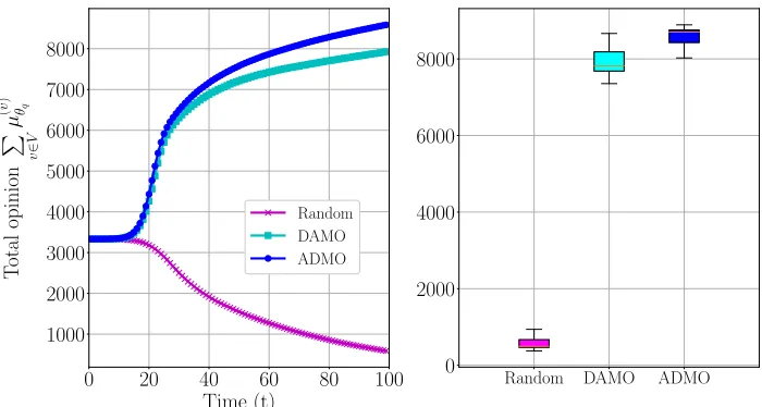
0 20 40 60 80 100 Time (t) 1000 2000 3000 4000 5000 6000 7000 8000 T ot al op in io n

P v∈

V µ ( v ) θq Random DAMO ADMO

Random DAMO ADMO

0 2000 4000 6000 8000

(a)Evolution of total opinion with time (left), and total opinion at time t=100 (right) for differ-ent algorithms in PA graph of 104 nodes.

0 20 40 60 80 100

P v∈

V µ ( v ) θq Random DAMO ADMO

Random DAMO ADMO

1000 1500 2000 2500 3000

(b) Evolution of total opinion with time (left), and total opinion at timet=100 (right) for differ-ent algorithms in Facebook ego-network.

(54)

Random ADMO

P

A graph

F

acebook ego-network

(a)Visualization of opinions in PA graph of 103nodes (top) and Facebook ego-network (bottom). Blue - affinity towards ˜θ, and green and red - affinity towards Θ∖θ˜.

t = 20 t = 30

t = 50

t = 100

(1,0,0)

(0,1,0) (0,0,1)

(1,0,0)

(0,1,0) (0,0,1)

(1,0,0)

(0,1,0) (0,0,1)

(1,0,0)

(0,1,0) (0,0,1)

(b) Evolution of beliefs at timet=20,30,50 and 100 (clock-wise), respectively, in PA graph of 103 _nodes.

(55)

and 104 _{nodes with the preferential attachment parameter} _m₌_{3. Facebook ego-network} consists of 4039 nodes with a high clustering coefficient (0.6055) and small diameter (8). There are 3 sources in the network, one of which employs the smart information spreading, while the rest spread information at random. The discount factors γ′ _and γ′′ are set to 0.95 and 0.97, respectively. The temperature T of Boltzmann exploration is

set to 0.015 for 103 _{nodes and 0.03 for 10}4 _{nodes. The parameters pertaining to the} communication model Psp, L and Rm are set to 0.1, 20, and 2, respectively. Finally, the

remembering factor β and the belief update parameter ζ are uniformly distributed for each node in [0.9, 1] and [0, 2], respectively. The parameters NQ and N are both set

to: 4 for PA graph with 103 _{nodes, and 5 for PA graph with 10}4 _{nodes and Facebook} ego-network. For the centralized algorithms, the number of samples NS = 20. All the

simulation results are averaged over 100 iterations. In our simulations, we evaluate the performances of the following: 1. Proposed algorithms: In this case, messages of node ˜v are spread in the network using one of the proposed algorithms, while the messages of the nodes in Vr are spread randomly. 2. Random baseline: Messages of all the sources

VS are pushed by the regular nodes in the network uniformly at random. Moreover, to

mimic the real-world scenario, in the simulations we consider that a node’s opinion is unaltered upon reception of duplicate messages.

2.6.1 Final Opinion and Centralities

We define the final opinion of a node to be its opinion at time T = 100. Figure 2.9a

(56)

current-Table 2.3 PCC for different choices of centralities.

Centrality

Current-flow closeness

Current-flow

betweenness

Betweenness Closeness Degree

PCC 0.77 0.66 0.60 0.45 0.64

flow closeness centrality [6] since it exhibits the highest correlation with the final total opinion. The Pearson correlation coefficient (PCC) for different choices of centralities is shown in Table 2.3. It can be observed that the average opinion of the nodes with smart information spreading is significantly greater than its random counterpart. We can also observe from the figure that even though a node is unfavourably located (away from hubs in PA graph), the opinion maximization can be achieved through smart information spreading using our proposed algorithms.

2.6.2 Opinion Evolution with time

Figure 2.9b depicts the evolution of the total opinion of the population with time for different variants of the proposed centralized and decentralized algorithms. The centrality of the smart source ˜v is 1.5×10−3. The order of performance can be observed as: ACMO > ADMO,CAMO > DAMO. It can be observed that using Q-learning based approach

improves the performance of the algorithms. Since, the beliefs are slowly varying with respect to time, Q-learning can be used to estimate the future reward up toNQtime steps

and actions can be chosen accordingly. Based on the application specific requirements, the decentralized algorithms can be used effectively due to their lower computational complexity. In larger networks (> 103 nodes), owing to the higher complexity of the

(57)

depicted. Figure 2.10a shows the evolution of total opinion with time corresponding to all the sources (smart and random) in a PA graph with 104 _{nodes. It can be observed} that the smart sources employing learning-based active information spreading process can polarize the opinion of the population, while the random sources influence only a small fraction of nodes. In Figure 2.10b, the evolution of total opinion and the final total opinion is depicted for the proposed algorithms in the Facebook ego-network with 4039 nodes along with the random baseline. The performance trend is similar to that of PA graphs as described earlier. Moreover, we can observe that the performance gap between DAMO and ADMO algorithms in the Facebook ego-network is larger than that in PA graph owing to the community structure of the Facebook ego-network, which is utilized by ADMO by penetrating outside the community for better rewards. Considerable improvement can be observed in the performance of the proposed algorithms over random spreading. Also, the average final total opinion of ADMO algorithm about 25 percent greater than that of DAMO algorithm.

Information Spreading in Dynamic Networks.

ABSTRACT

DEDICATION

BIOGRAPHY

ACKNOWLEDGEMENTS

TABLE OF CONTENTS

LIST OF TABLES

LIST OF FIGURES

Chapter 1

Introduction

1.1

Smart information spreading for opinion

maxi-mization in networks

1.1.1

Motivation

1.1.2

Related Work

1.2

Dynamic advertising in VANETs using repeated

auctions

1.2.1

Motivation

1.2.2

Related Work

1.3

Information spreading in time-varying networks

1.3.1

Motivation

1.3.2

Related Work

1.4

Background

1.4.1

Dirichlet Distribution

1.4.2

Dynamic Bayesian Networks

1.4.3

Network Models

1.4.4

Gossip-based Information Spreading

Chapter 2

Smart Information Spreading for

Opinion Maximization in Social

Networks

2.1

System Model

2.1.1

Network Model

2.1.2

Communication Model

2.1.3

Evolution of Opinions

2.2

Problem Formulation

2.2.1

A Toy Example of Opinion Maximization

x

y

c

d

c

d

x

y

Number of samples (

N

)

E

{

r

}

2.2.2

Representation of Opinion Evolution in the Network as a

Dynamic Bayesian Network

2.2.3

From DBN to Influence Diagram

X

Ω

X

A

_E[g(X