Physical Match
Aaron E. Naiman, Eliav Farber and Yossi Stein
Department of Applied Mathematics, Jerusalem College of Technology-Machon Lev, Jerusalem, Israel E-mail: [email protected]
Keywords: physical match, curve matching, pattern recognition, edge pixels, image processing, curve fitting, cyclic, longest common subsequence
Received:September 13, 2017
We present an approach to solving the problem of “physical match,” i.e., reconnecting back together broken or ripped pieces of material. Our method involves correlating the jagged edges of the pieces, using a modified version of the longest common subsequence algorithm.
Povzetek: Predstavljena je izvirna metoda sestavljanja razbitih fiziˇcnih predmetov.
1
Introduction
The problem of “physical match” spans many different ap-plications, from whimsical (jigsaw) puzzle solving [9, 19, 20], to 3-D archeology [17, 14, 7, 6] (sometimes utilizing a priori shape knowledge, or rotational symmetry), to the forensic sciences [15, 16]. In the present paper we restrict ourselves to the 2-D problem, and the particular aspects of one-dimensional border which one can take advantage of, for this flat case, but not resorting to the rich information of 3-D surface-to-surface matching. Therefore, given a single piece of material, be it paper, clothing, glass, etc., once it is ripped or broken into many pieces, the challenge is to piece back together the parts, to the original shape.
Sometimes one can take advantage of text [18], color [9], orientation (e.g., lined paper), images [20, 10, 4], spe-cific shapes (e.g., machine-shredded paper [18], or the jig-saw puzzle problem [19]) and/or texture. A survey of such methods can be found in [8]. We are making none of these assumptions, and therefore matching via shape alone.
Some approach this problem with gross polygon approx-imations of the pieces [1], whereas others solve with a mul-tiscale of resolutions [3]. Our method is based on cor-relating the changes of direction along the edges of the pieces. In [21], the same information is used, however, whereas they build histograms of these changes of direc-tion, we compare them directly, retaining their order, as described below. Finally, [16] present statistical findings (for the plausibility of the Daubertruling in the court of law) for three different types of material. Our analysis is for generic materials, and we concentrate more on the al-gorithms involved.
2
Background and problem
We have chosen to, at least initially, model the pieces on the computer, rather than work with actually torn material. The reason for this is in order to steer away from
possi-ble parameter fixing based on a few physical cases, and instead deriving statistics and parameter values, based on thousands of computer-modeled Monte-Carlo simulations. In order to accurately match along the edges of the pieces, we start by scanning in the pieces to determine the location of all of the edges. This has to be done with enough resolution to pick up the unique characteristics of each segment of the edge, and minimize the effects of the jagged nature of digitization of the edge pixel positions. On the other hand, the resolution cannot be too high, lest the computations be inordinately expensive.
Once the edges have been located, the edge slopes have to be calculated in such a fashion so that they can be com-pared to each other. The slope calculations require an or-deringof the pixels, which is accomplished together with the previous step of locating the edge pixels. This is done for all of the edges of all of the pieces. Since the pieces have been translated and rotated with respect to each other, we actually stored away in arrays, one for each piece, the invariantchangesin direction along the edge. This we are able to accomplish, as we “travel” along the edges (ex-plained below), recording the rotations.
After the edges have been characterized, the core of our system is to find where the turns of the edges of separate pieces correctly match up. We use a modified version of the longest common subsequence (LCS) algorithm [5], ad-justed to be appropriate for problems where the starting points of the sequences are not known.
Finally, the last step is to calculate from the matching turns, where exactly to “sew” the pieces back together. This stage requires further filtering of the matching algorithm, to dispose of spurious matches along the edges.
To summarize, the following algorithms are needed for us to model and verify our physical match system:
1) modeling original, non-trivial pieces of material, and breaking them further into pieces,
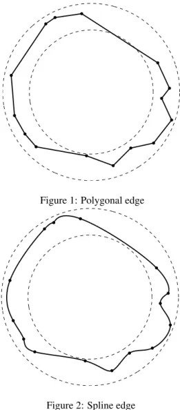
cally circular in shape, but we perturb the edge to obtain a polygon. Beginning with a center, we randomly choose a sequence of angles, as well as radii, ranging between two given extrema. These points are then connected with straight lines to obtain the polygon. See an example of this in Figure 1. A less-simple shape would be to connect the same points with splines, as seen in Figure 2. The
ramifi-Figure 1: Polygonal edge
Figure 2: Spline edge
cations of such a shape on the subsequent algorithms, will be the subject of future analysis.
Figure 3: Break exiting polygon
Figure 4: Two pieces
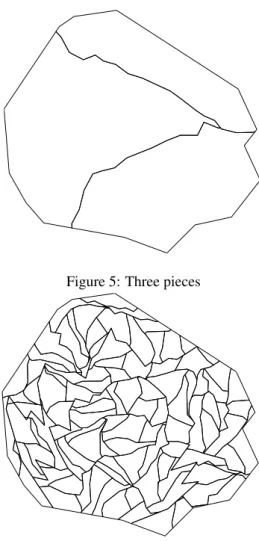
Treating each sub-piece separately, we can now recurse, breaking each piece further and further. Examples of 3 pieces and 100 pieces are shown in Figures 5 and 6.
When determining the values of the extrema, both for the random direction and the random length of the step we take, it is important to generate a break with similar “turn” characteristics to the original polygon edge.
The reason for this is the following. While it is true that, e.g., for a simply-shaped piece of material, the break may actually generate a different kind of edge, we are look-ing for a worst-case scenario, where we cannot easily tell where the ripped part is, and where the original polygonal edge is. Two counterexamples can be seen in Figures 7 and 8.
poly-Figure 5: Three pieces
Figure 6: One hundred pieces
gon, as is the case on the left hand side of Figure 9. This is because the segment may actually leave the polygon, but subsequently return back into it, as in the right hand side of the same figure.
We therefore check at each step of the break, whether the new step segmentintersectsany part of the edge of the polygon. If it does, we set the end of the break at the inter-section point.
Finally, future analysis will study possibilities where the break is also generated with splines.
With the pieces now “virtually” created, we are ready to start our analysis. We will now discuss the rasterization of the images, in order to simulate their being scanned “back” into the computer, for running our physical match system.
4
Image scanning and edge pixel
ordering
In real life, the entire process starts here, from scanning the pieces into the computer. At this point, a mesh of pixels representing each piece is available, with each pixel signi-fies where the piece is, or is not. For our analysis, this is a best-case segmentation of the material (not always
eas-Figure 7: Complex break
Figure 8: Simpler break
Figure 9: Breaking out of piece
ily obtainable), into foreground (where the material is) and background (where it is not). The next step is to discover which theedgepixels are, and to determine an ordering of them, for subsequent edge slope calculations.
In the model we built in the previous section, the situa-tion is slightly different. There we already have a polygon defined, and we need to determine which of the pixels are edge pixels, as well as a proper ordering for them. To best simulate real life, we first rotate and translate each piece, as well as randomly choose whether or not to flip each piece over.
edge pixel discovery and ordering.
5
Edge slope calculations
Given an ordering of edge pixels, we now need to calculate the edge slope at each pixel. This will subsequently be used for calculating the edge slope differences, needed for matching between pieces.
While an accurate edge slope calculation would be suffi-cient, it is not necessary. We need an approximation of the edge slope which will be both reproducible, and invariant (to a given degree of tolerance) under rotation and transla-tion. With this characterization, we will be able to match the (changes of) slope of two different pieces, regardless of translation and rotation.
The authors demonstrate in [12] that the method of a linear least squares (LLS) fit to a parabola, accurately calculates this reproducable, rotation- and translation-independent characterization of the edge slope. (LLS fits to other orders of polynomials, were shown to be inferior.) Note that care needs to be taken so that the initial scanning supplies a high enough resolution. This will enable enough points to be supplied to the LLS fit so that no more than one “turn” will be present in each set of points. (The de-gree to which a “turn” is rendered significant, as well as the number of points per turn, are empirically derived in that paper.)
As they describe, the problem is not trivial, due to the el-ement of rotation-invariance, where in the local neighbor-hood, a very different set of pixels represents the same edge segment. Nonetheless, after implementing their method, we have for each piece an array of edge slope values, one value for each edge pixel.
6
Matching edges
The matching between pieces is done on a one-to-one basis. That is, each of the pieces is compared with every other piece, in order to determine the best match.
Since the pieces are rotated vis-à-vis each other, there is no reason to find matches between edge slope values. How-ever, thechangesin edge slope are invariant to rotation. As
case) or nearly straight lines. Therefore, the edge slope values for many adjacent edge pixels may be nearly equal, and their differences will be zero or close to it.
While these straight edge segments can represent impor-tant information, our current algorithm matches based on
changes in edge slope directions. Therefore, with all of these zeros left in the arrays, too much “straight-edge” in-formation will match, not uncovering the underlying turn-information.
Deleting all such zeros removes too much information, and therefore our current algorithm replaces multiple adja-cent zeros with a single zero, as a place marker stating that there was a straight stretch of edge here.
Whereas one might think that quantitative information is lost here, since nolengthof the straight edges is retained, nonetheless cases of unequal length will properly be fil-tered out later on, when the pieces are attempted to be sewn together (Section 7).
6.2
Relative orientation
If the edge values of one piece are ordered in the exact op-posite direction with respect to the other piece, then the changes in edge slope values of one piece are the negative values of the other piece, in addition to being in the oppo-site order.
For example, the edge on the left hand side of Figure 10 shows moving from one edge pixel to the next one is a90◦
Figure 10: Pixels in reverse direction
Similarly, if one piece is flipped over as compared to the other piece, then the values will be either in the opposite order (−30◦,90◦), as in Figure 11,orwith reversed signs
Figure 11: Flipped piece with opposite order
(90◦,−30◦), as seen in Figure 12.
Figure 12: Flipped piece with reversed signs
Therefore, we need to compare the two array in four dif-ferent fashions:
1) as is,
2) with one of the arrays reversed,
3) with one of the arrays with opposite signs and
4) with one of the arrays reversed and with opposite signs.
6.3
Cyclic correlation
Recall that each array represents the changes of edge slope values for the perimeter of a given piece. Since we ran-domly choose where along an edge to start the array, we do not know where a matching segment is for any two pieces. It could be that the match is in the middle of arrayA, but for arrayB, it is at the end of the array, and finishes subse-quently back around at the beginning of the array.
The authors in [11] deal with this issue at length and demonstrate that initially four LCS algorithm invocations are necessary:
1) as is,
2) with one array rotated by 50%,
3) with the other array rotated by 50% and
4) with both arrays rotated by 50%.
(Rotating the array amounts to choosing a different start-ing point along the piece’s edge.) Paddstart-ing the array with the same content was avoided, in order to avoid possible spurious artifacts.
Note that these four possibilities are in addition to the four permutations mentioned previously in Section 6.2, with reversed arrays and negative values. Therefore, the composite set of possibilities includes a total of 16 pos-sibilities. The best LCS (of the 16) is found, and then if deemed necessary, one or both arrays are reversed, sign-changed and 50% rotated.
In the same paper, the authors show that once the best LCS (so far) is found, and after performing a centering technique they devised, an additional invocation of the LCS algorithm is necessary to extract the LCS. They establish that for cases where the LCS in the two sequences are known to be clustered within the sequences, this final cen-tering and subsequent LCS algorithm step provide optimal LCS results.
Our problem indeed exhibits this clustering behavior, as two pieces generally match along the adjacent side, and not all the way around. (A degenerate case is when one piece sits totally within another.)
With the two LCSs lined up and centered within their sequences, we are ready to proceed with the final stage of “reconnecting” the two pieces back together.
7
Sewing edges
As was noted in the previous section, a final invocation of the LCS algorithm was used in order to extract an LCS as long as possible. However, even with optimal results of obtaining the entire, appropriate LCS, we still need to concern ourselves with spurious, random matches which may enter the LCS.
7.1
Filtering random matches
Consider Figure 13. We see that although we have a good
Figure 13: With spurious matches - both sides
match overall, if we are to consider the extra, spurious cir-cled matches which areoutsideof our match, this might se-riously degrade our subsequent calculations for reconnect-ing the pieces.
7.2
Moving and rotating
We must first move the two pieces next to each other, in order to enable the final stitching. For simplicity’s sake, we assume one piece to be stationary, and the other will be matched up to it. Since this second piece is both trans-lated away, and rotated from the first piece, the following maneuver will return its coordinates[x y]T to their correct locations:
cosα sinα −sinα cosα
x y
+
∆x ∆y
The challenge, therefore, is to find the optimal values ofα, ∆xand∆y, to juxtapose the two pieces.
Even though we have already established our matching positions within the arrays, along with their (x, y) coor-dinates, we acknowledge sources of initial measurement errors in the scanning, as well as possible internal mis-matches, mentioned above. We therefore use a nonlinear least squares (LSQ) solver (in MATLAB: lsqnonlin) to find the triad of values which minimizes the sum of the square distances between our remaining LCS matches. Note: as many nonlinear solvers require, we initially seed the solver with a seat-of-the-pants approximation given the geometry and any three matching pairs. Also, it was cru-cial to adjust the maximum number of iterations allowed (in MATLAB:MaxIter) and the termination tolerance on x (MATLAB: TolX) in order to converge properly to the desired results.
7.3
Micro-stitching
With our two pieces lined up next to each other, we have the situation shown in Figure 14. We need to find the en-tire “seam” in order to properly stitch the two pieces to-gether. A proper stitching is crucial for the success of fur-ther matching to more pieces. Note that now we would like to find the most number of pixels which can be considered part of the seam, with the remaining pixels comprising the edge of the combined piece. Therefore, matching between pixels of the two pieces:
1) entails geometric proximity, instead of matching slopes as before, and
Starting from the LCS center, the algorithm proceeds in both directions along the seam, by adding the closest pixels (to each other) from the two pieces, as long as their distance is 0.4 of the average mean distance (calculated earlier in the nonlinear least squares procedure). We allow skipping pixels, as long as subsequent ones are part of the seam. When we hit three consecutive pairs which are too far apart, we consider the seam ended (in that direction). Note that the 0.4 value and the count of three consecutive pairs, were empirically derived.
7.4
Goodness of fit
Due to the digitized nature of the problem, we need metrics to measure the quality of the matches. The minimized sum squared error calculated to translate and rotate the pieces gives us one measure, but that was prior to the stitching.
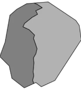
We therefore measure the overlap between the two pieces, as well as gaps which may have been uncovered. See, e.g., in Figure 15, where the dark gray area near the
Figure 15: Overlap and gap
top shows us the overlap, and the thin light gray strip to-wards the bottom—where neither piece covers.
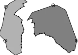
of Figure 16 we see that although our eyes solve the
prob-Figure 16: Reconfigurable pieces
lem easily, moving the two pieces together, another pos-sibility can be seen as well, on the right hand side of the figure. Note that the latter possibility suffers no overlaps or gaps, along the seam.
Clearly this is not the desired result. We therefore run a quick, low-resolution scan of the union of the two pieces, discarding this possibility by comparing the total area be-fore and after stitching. Note that one cannot decide on a consistent ordering of the edge pixels based on concav-ity/convexity of the pieces, as even along matching edges, part of the shared edge might be concave, and part convex. One final measure of fit, is the length of the seam. This is needed, as, e.g., if two pieces meet at just one point, then the sum squared error will be zero, there will be no overlap nor gap areas, and the area of the union will be exactly equal to the sum of the individual areas. However, the seam length will be zero too, indicating that no match at all occurred.
The gross overlap demonstrated in Figure 16, and the extremely short length of the seam, are not used statistically with the first two metrics, i.e., the lengths of overlaps and gaps. These last two measures of fit used in a binary fashion to throw away possible matches.
8
Results
We present here some sample cases, together with empirically-drawn heuristics regarding system parameter values.
8.1
More than two pieces
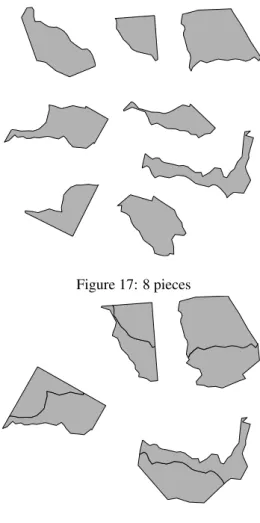
When we start with more than two pieces, we compare ev-ery piece to evev-ery other one. We take the “greedy” ap-proach of choosing the candidate pairs which maximize the number of possible “sewings,” for this round of the physical match. Others [10, 4] approach this by building graphs of matches, subsequently redivided into subgraphs by spectral clustering.) E.g., if the following pairs have been discovered: (1,2), (2,3) and (3,4), we will ignore the (2,3) match, first working with the other two pairs. Once that is finished, we iterate until all possible matches have been found. See Figures 17–21.
8.2
System parameter values
Our entire approach is subject to a number of interdepen-dent, system-level parameters which need to be set to the
Figure 17: 8 pieces
Figure 18: 8 pieces stitched
correct values. We demonstrate below what can happen with the wrong set of values.
The parameters of interest are:
Resolution This is the scanning resolution of the various pieces into the computer, in MATLABpixels. As men-tioned in Section 5, care needs to be taken so that the resolution is high enough to capture the twists and turns of the edge, but not too high, as to make the com-putation inordinately long. Sample values (in MAT
-LABcoordinates): 100, 200.
Edge characterization points Again, as discussed in the same section, this needs to be large enough to supply the linear least squares fit to a parabola algorithm with enough information to characterize the edge slope, but not too large, so that no more than one turn is present in the set of points. Sample values: 23–29 (resolution of 100), 31–37 (resolution of 200).
Figure 20: 4 pieces stitched
Figure 21: 2 pieces
LCS maximum match In the LCS matching algorithm, we stated in Section 6 that when comparing changes of slope, we are willing to have these numbers be dif-ferent, up to this maximum value. Sample values: 0.1–0.4.
LSQ confidence in matches This value is used in Sec-tion 7.2 to supply the nonlinear least squares fit with matches, to translate and rotate the pieces together. It is a fraction of the matches in each direction, starting from the center of the LCS. Sample values: 0.10–0.25.
In addition to the conclusions we derive below, we found:
1) Overall it makes sense to scan at a resolution of 200, in order to obtain better fit statistics (preventing overlaps and gaps), which in turn provides better conditions for subsequent matches to other pieces.
2) The LSQ confidence in matches parameter was less important.
3) Of the three remaining parameter: edge characteriza-tion points, straight corner maximum and LCS
max-In general, the values in Table 1 worked optimally for a
resolution of 100 edge characterization points 27, 29
straight corner maximum 0.4–0.8 LCS maximum match 0.2–0.4 LSQ confidence in matches 0.10–0.25
Table 1: Resolution of 100 — optimal values
scanning resolution value of 100. We show in Table 2 the
resolution of 200 edge characterization points 35, 37
straight corner maximum 0.4–0.8 LCS maximum match 0.2–0.4 LSQ confidence in matches 0.10–0.25
Table 2: Resolution of 200 — optimal values
optimal valus for a scanning resolution value of 200. We present here a specific case, in order to illustrate what happens when the system parameters stray too far from the nominal values. In Table 3 are the system parameter
val-resolution of 100 edge characterization points 25
straight corner maximum 0.8 LCS maximum match 0.2 LSQ confidence in matches 0.20
Table 3: Nominal values
ues for this specific case. The subsequent matches are dis-played in Figure 22, showing a good match up between the two pieces.
Figure 22: Nominal values
Figure 23: Edge characterization points too low
correct seam, but all around the edges.
Another problematic case is if the straight corner maxi-mum is set too low. In Figure 24, with the value set to 0.3, we see that onlyverystraight corners are considered to be modeling straight lines, and therefore we have a huge num-ber of matches. The information at the corners of interest is lost in the noise.
Finally, we demonstrate what happens if the LCS max-imum match system parameter is set too low. A value of 0.01 is too stringent to allow edge slope changes of the two pieces to match up with each other. This is seen in Fig-ure 25, where very few matches have been established.
Figure 24: Straight corner maximum too low
Figure 25: LCS maximum match too low
9
Future research
We list here a number of future directions for this research.
1) As mentioned in Section 3, we would like to build the initial piece, as well as generate the breaks, using the more general splines, instead of straight lines.
2) Clearly we would like to run the analysis for actual pieces of broken/torn material, in order to verify the optimal system parameter values.
3) “Holes” in the material might be due to missing pieces. How do the holes effect this process? Can the stitching algorithm of Section 7.3 easily be modi-fied so as to be able to “jump” over such holes? Note that previous work of automating jigsaw puzzle recon-struction rarely addressed this.
4) In addition, we would like to understand how various types of material (glass, pottery, plastic, rubber, etc.) effect the system parameter values of choice.
5) Specifically, paper has more characteristics, due to the fibers jutting out along the torn edge. Can we take advantage of these? Are they “in the way?” Can we remove them, without effecting the success of the sub-sequent matching?
6) On the issue of paper, how does the fact that it is usu-ally multi-ply, effect the analysis? Can we analyze each ply, and match on the composite picture?
7) This also brings us to the exciting extension to 3-D physical match, with applications to archeology and exploded object reconstruction.
8) Finally, there is the area of forensics. In order to claim: “This piece came from this object.” and have this be admissable in court, we have to answer ques-tions regarding confidence levels of the fit, as well as statistical probability that no other piece could likely fit there.
10
Summary
We have presented a method for solving the problem of physical match. The algorithm involves finding the edge pixels, ordering them, and using their positions to char-acterize the edge slope. The turns along the edges are then matched to each other using a modified version of the longest common subsequence algorithm.
Finally, the various pieces are translated, rotated and flipped (if necessary), and then stitched together for further matching to other pieces.
We discussed future directions for the research, particu-larly in the arena of extending the analysis to 3-D shapes and breaks.
References
[5] M. R. GAREY AND D. S. JOHNSON, Computers and Intractability: A Guide to the Theory of NP-Completeness, W. H. Freeman, 1979.
[6] Q.-X. HUANG, S. FLÖRY, N. GELFAND, M. HOFER, AND H. POTTMANN, Reassembling fractured objects by geometric matching, in ACM Transactions on Graphics (TOG), vol. 25, ACM, 2006, pp. 569–578.
[7] M. KAMPEL AND R. SABLATNIG, 3d puzzling of archeological fragments, in Proc. of 9th Computer Vision Winter Workshop, vol. 2, Slovenian Pattern Recognition Society, 2004, pp. 31–40.
[8] F. KLEBER AND R. SABLATNIG,A survey of tech-niques for document and archaeology artefact recon-struction, in Document Analysis and Recognition, 2009. ICDAR’09. 10th International Conference on, IEEE, 2009, pp. 1061–1065.
[9] D. A. KOSIBA, P. M. D.AND. S. BALASUBRAMA
-NIAN, T. L. GANDHI,AND K. KASTURI,An auto-matic jigsaw puzzle solver, in Proceedings of the 12th IAPR International Conference on Pattern Recogni-tion - Conference A: Computer Vision & Image Pro-cessing, vol. 1, 1994, pp. 616–618.
[10] H. LIU, S. CAO,AND S. YAN,Automated assembly of shredded pieces from multiple photos, Multimedia, IEEE Transactions on, 13 (2011), pp. 1154–1162.
[11] A. E. NAIMAN, E. FARBER,ANDY. STEIN,CLCS— cyclic longest common subsequence, 2018. submit-ted.
[12] , Edge characterization of digitized images, Oct. 2018. submitted.
[13] , EdgeTrek—interior and boundary pixels for large regions, Oct. 2018. submitted.
[14] G. PAPAIOANNOU AND E.-A. KARABASSI, On the automatic assemblage of arbitrary broken solid artefacts, Image and Vision Computing, 21 (2003), pp. 401–412.
Y. KOMPATSIARIS, AND M. G. STRINTZIS, Shred-ded document reconstruction using MPEG-7 stan-dard descriptors, in Proceedings of the Fourth IEEE International Symposium on Signal Processing and Information Technology, Dec. 2004, pp. 334–337.
[19] H. WOLFSON, E. SCHONBERG, A. KALVIN1,AND
Y. LAMDAN, Solving jigsaw puzzles by computer, Annals of Operations Research, 12 (1988), pp. 51– 64.
[20] F.-H. YAO AND G.-F. SHAO, A shape and image merging technique to solve jigsaw puzzles, Pattern Recognition Letters, 24 (2003), pp. 1819–1835.