Hai Liu, Yong Feng, Qian Qian and Bin Zhang
Yunnan Key Laboratory of Computer Technology Applications, Kunming University of Science and Technology, Kunming, China
Constructing Reliable Virtual
Backbones in Probabilistic Wireless
Sensor Networks
Most existing algorithms used for constructing virtual backbones are based on the ideal deterministic network model (DNM) in which any pair of nodes is either fully connected or completely disconnected. Different from DNM, the probabilistic network model (PNM), which presumes that there is a probability to connect and communicate between any pair of nodes, is more suitable to the practice in many real applications. In this paper, we propose a new algorithm to construct reliable virtual backbone in probabilistic wireless sen-sor networks. In the algorithm, we firstly introduce Effective Degree of Delivery Probability (EDDP) to indicate the reliable degree of nodes to transfer data successfully, and then exclude those nodes with zero EDDP from the candidate dominator set to construct a reliable connected dominating set (CDS). Moreover, each dominatee selects the neighbor dominator with the maximum delivery probability to transfer data. Through simulations, we demonstrate that our pro-posed algorithm can remarkably prolong the network lifetime compared with existing typical algorithms. ACM CCS (2012) Classification: Networks → Net-work algorithms → Control path algorithms → Net-work design and planning algorithms
Networks → Network types → Ad hoc networks → Mobile ad hoc networks
Networks → Network performance evaluation →
Network simulations
Keywords: probabilistic wireless sensor networks, virtual backbone, reliable connected dominating set, delivery probability
1. Introduction
Wireless sensor networks (WSNs) are emerg-ing as the desired environment for increasemerg-ing numbers of military and civilian applications,
such as disaster control, environment and hab-itat monitoring, battlefield surveillance and health care applications [1], [2]. Sensor nodes usually use battery power, and thus their energy is very limited and not easily replenished. The energy scarcity of sensor nodes significantly limits the lifetime and performance of wireless sensor networks [3], [4]. Simultaneously, for the infrastructure-less and dynamic topology features, many routing protocols usually cause broadcasting storm in WSNs, which aggravates the energy consumption of nodes [5]. Sensor nodes deployed in the field can't be recharged to retain their energy resources; hence energy efficiency is a major issue in WSNs [6].
of nodes are not fully connected but reachable via the so called lossy links. As reported in [8], there are often much more lossy links than fully connected links in a WSN. Therefore, a more practical network model for WSNs is the prob-abilistic network model (PNM).
In PNM, there is a delivery probability as-sociated with each link connecting a pair of nodes, which is used to indicate the possibil-ity of successfully transmitting packages on the link. In order to guarantee the reliability of the virtual backbone, it is reasonable to select the links with higher delivery probability. In recent years, there have been some algorithms for con-structing reliable virtual backbones in PNM, e.g., constructing a reliable minimum-size CDS (MCDS) [9], a load-balanced virtual backbone [10] and a reliable topology control in the whole network [11]. However, these algorithms do not take the reliability of dominators into account, and thus do not guarantee the reliability of the constructed virtual backbone.
In this paper, we propose a new algorithm to construct Reliable Virtual Backbone in PNM by constructing a reliable CDS (RVBP-CDS). Particularly, the main contributions of this pa-per are summarized as follows:
(i) We propose a new algorithm to construct a reliable virtual backbone in probabilistic wireless sensor networks. The core idea of the algorithm is preferentially to improve the reliability of the links between domina-tors, and then improve the reliability of the links between dominators and dominatees. (ii) We introduce some new concepts in our
algorithm, e.g., delivery probability rank to indicate the rank of delivery probabil-ity between a node and its neighbor nodes; effective degree of delivery probability to ensure the number of effective neighbor nodes.
(iii) We propose a new method to construct a reliable CDS, in which the nodes which have the higher EDDP and delivery prob-ability are preferentially selected as domi-nators.
The rest of this paper is organized as follows. In Section 2, we review some related literature on DNM and PNM, analyze its advantages and dis-advantages. In Section 3, we introduce the
net-work model and delivery probability, formally define some concepts under PNM. The design of the RVBP-CDS algorithm is presented in Section 4. The simulation results are presented in Section 5 to validate our proposed algorithm. Finally, the paper is concluded in Section 6.
2. Related Work
The ideal deterministic network model (DNM) has been widely used in most existing algo-rithms for constructing virtual backbone and the connected dominating set is a good way to build the virtual backbone.
The authors in [12] proposed an algorithm for constructing the virtual backbone by construct-ing a connected dominatconstruct-ing set. In this paper, dominator nodes are selected according to the number of neighbor nodes. Each node is ini-tially colored white. Next, the node with the largest degree is colored black and all its neigh-bors are colored gray. This last step is repeated until there are no white nodes left in the graph. Each time, the gray node with the largest num-ber of white neighbors is colored black and then all its white neighbors are colored gray. Node IDs can be used to break ties. Finally, all black nodes form a CDS. Since this CDS is also of minimal size, it is called MCDS. The MCDS can cause a single dominator with more con-nected dominatees to consume energy faster than other dominators.
In order to solve the unbalance-load problem, in [12], J. He et al. proposed an algorithm for con-structing a load-balanced virtual backbone [13]. For achieving the purpose of load balancing about the whole network, there are two parts of work. The first part of the work is to construct a CDS with the minimum p-norm value in order to assure that the workload among each domi-nator is balanced. The second part of the work aims to load-balancedly allocate each domina-tee to a dominator.
There are a lot of other algorithms to construct the virtual backbone, [14] proposed a grid par-titioning algorithm for constructing the virtual backbone. The algorithm divides the whole area of the network into virtual grids. The virtual grid is defined such that, for any two adjacent grids, any node in one grid can directly
commu-between each dominator and its dominatees, using the sum of the two probabilities as the gene in the multi-objective genetic algorithm. They use the binary tournament to select as the virtual backbone the best individual set, which is a CDS. However, the above method does not provide a good consideration of the link reliability of the constructed virtual backbone when used as the main data transmission chan-nel. However, as dominators build the main data transmission channel in the network, the algorithm can't ensure that dominators have the highest reliability.
However, all of the abovementioned algo-rithms in probabilistic network model (PNM) have never considered the maximum reliability of dominators. Dominators are the main data transmission channel in the network. If we sure the reliability of dominators, we will en-sure the reliability of the whole network. In this paper, we preferentially consider the reliability of dominators, and then we improve the reli-ability between dominators and dominatees to the utmost extent.
3. Network Model and Problem
Definition
3.1. Network Model
The definition of network model in probabilis-tic network model (PNM) is given here. Under the PNM, we model a WSN as an un-directed graph G(V,E,γ(E)), where V is the set of n
nodes, denoted by vi, where 0 ≤ i ≤ n, i is called the node ID of vi in the paper. E is the set of lossy links. ∀ vi, vj∈V, there exists a link (vi, vj) in G if and only if:
(i) vi and vj are in each other's transmission range and
(ii) γij > 0.
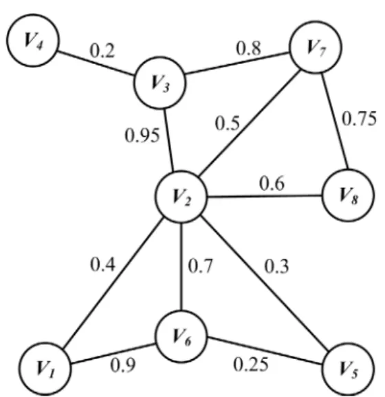
For each link (vi, vj) ∈E, γij indicates the proba-bility that node vi can successfully and directly deliver a packet to node vj, and γ(E) = {γij| (vi, vj) ∈E, 0 < γij ≤ 1}.We assume that the links are undirected (bidirectional), which means that two linked nodes are able to transmit and receive information from each other with the same γij value [10]. Figure 1 presents an exam-ple of network model in this paper.
nicate with any node in the other grid, and then choose a dominator in each virtual grid to form the virtual backbone. The work also proposed a state transition to change different node in ac-tive state to prolong the network lifetime. But the grid partitioning algorithm for constructing virtual backbone has a distinct disadvantage, which is that it can't guarantee the number of nodes in a grid, if the number of nodes in a grid is too little, it will reduce the whole network lifetime. Another disadvantage is that it can't guarantee the number of dominators to achieve the optimal.
In probabilistic network model, the algorithms for constructing the virtual backbone mainly include the following. A huge amount of ap-proximation algorithms have been proposed to construct an MCDS-based VB, which is a well-known nondeterministic polynomial time (NP)-hard problem [15]. So we can only pray for an approximate solution. In [9], the author proposed a genetic algorithm for constructing a reliable MCDS in probabilistic wireless net-works. Its reliability is above a preset applica-tion-specified threshold. The algorithm works mainly through using a fitness function to find a minimum-sized CDS whose reliability should be greater than or equal to a preset threshold. However, we can see that the reliability of CDS decreases while increasing number of dom-inators, i.e., increasing size of CDS, and the MCDS may cause single dominator which has more connected dominatees consumes its en-ergy much faster than other dominators.
In [10], the authors proposed an algorithm for constructing a load-balanced virtual backbone in probabilistic wireless sensor networks via multi-objective genetic algorithm. On the basis of the original minimum connected dominating set, through the operation of mating and muta-tion in genetic algorithm to generate new con-nected dominating sets, the authors use dom-inating tree to select the load-balanced virtual backbone by comparing multi-objective fitness function. However, in the full text, the authors don't guarantee the reliability of the virtual backbone, which may reduce the network life-time and increase the delay of network.
of nodes are not fully connected but reachable via the so called lossy links. As reported in [8], there are often much more lossy links than fully connected links in a WSN. Therefore, a more practical network model for WSNs is the prob-abilistic network model (PNM).
In PNM, there is a delivery probability as-sociated with each link connecting a pair of nodes, which is used to indicate the possibil-ity of successfully transmitting packages on the link. In order to guarantee the reliability of the virtual backbone, it is reasonable to select the links with higher delivery probability. In recent years, there have been some algorithms for con-structing reliable virtual backbones in PNM, e.g., constructing a reliable minimum-size CDS (MCDS) [9], a load-balanced virtual backbone [10] and a reliable topology control in the whole network [11]. However, these algorithms do not take the reliability of dominators into account, and thus do not guarantee the reliability of the constructed virtual backbone.
In this paper, we propose a new algorithm to construct Reliable Virtual Backbone in PNM by constructing a reliable CDS (RVBP-CDS). Particularly, the main contributions of this pa-per are summarized as follows:
(i) We propose a new algorithm to construct a reliable virtual backbone in probabilistic wireless sensor networks. The core idea of the algorithm is preferentially to improve the reliability of the links between domina-tors, and then improve the reliability of the links between dominators and dominatees. (ii) We introduce some new concepts in our
algorithm, e.g., delivery probability rank to indicate the rank of delivery probabil-ity between a node and its neighbor nodes; effective degree of delivery probability to ensure the number of effective neighbor nodes.
(iii) We propose a new method to construct a reliable CDS, in which the nodes which have the higher EDDP and delivery prob-ability are preferentially selected as domi-nators.
The rest of this paper is organized as follows. In Section 2, we review some related literature on DNM and PNM, analyze its advantages and dis-advantages. In Section 3, we introduce the
net-work model and delivery probability, formally define some concepts under PNM. The design of the RVBP-CDS algorithm is presented in Section 4. The simulation results are presented in Section 5 to validate our proposed algorithm. Finally, the paper is concluded in Section 6.
2. Related Work
The ideal deterministic network model (DNM) has been widely used in most existing algo-rithms for constructing virtual backbone and the connected dominating set is a good way to build the virtual backbone.
The authors in [12] proposed an algorithm for constructing the virtual backbone by construct-ing a connected dominatconstruct-ing set. In this paper, dominator nodes are selected according to the number of neighbor nodes. Each node is ini-tially colored white. Next, the node with the largest degree is colored black and all its neigh-bors are colored gray. This last step is repeated until there are no white nodes left in the graph. Each time, the gray node with the largest num-ber of white neighbors is colored black and then all its white neighbors are colored gray. Node IDs can be used to break ties. Finally, all black nodes form a CDS. Since this CDS is also of minimal size, it is called MCDS. The MCDS can cause a single dominator with more con-nected dominatees to consume energy faster than other dominators.
In order to solve the unbalance-load problem, in [12], J. He et al. proposed an algorithm for con-structing a load-balanced virtual backbone [13]. For achieving the purpose of load balancing about the whole network, there are two parts of work. The first part of the work is to construct a CDS with the minimum p-norm value in order to assure that the workload among each domi-nator is balanced. The second part of the work aims to load-balancedly allocate each domina-tee to a dominator.
There are a lot of other algorithms to construct the virtual backbone, [14] proposed a grid par-titioning algorithm for constructing the virtual backbone. The algorithm divides the whole area of the network into virtual grids. The virtual grid is defined such that, for any two adjacent grids, any node in one grid can directly
commu-between each dominator and its dominatees, using the sum of the two probabilities as the gene in the multi-objective genetic algorithm. They use the binary tournament to select as the virtual backbone the best individual set, which is a CDS. However, the above method does not provide a good consideration of the link reliability of the constructed virtual backbone when used as the main data transmission chan-nel. However, as dominators build the main data transmission channel in the network, the algorithm can't ensure that dominators have the highest reliability.
However, all of the abovementioned algo-rithms in probabilistic network model (PNM) have never considered the maximum reliability of dominators. Dominators are the main data transmission channel in the network. If we sure the reliability of dominators, we will en-sure the reliability of the whole network. In this paper, we preferentially consider the reliability of dominators, and then we improve the reli-ability between dominators and dominatees to the utmost extent.
3. Network Model and Problem
Definition
3.1. Network Model
The definition of network model in probabilis-tic network model (PNM) is given here. Under the PNM, we model a WSN as an un-directed graph G(V,E,γ(E)), where V is the set of n
nodes, denoted by vi, where 0 ≤ i ≤ n, i is called the node ID of vi in the paper. E is the set of lossy links. ∀ vi, vj∈V, there exists a link (vi, vj) in G if and only if:
(i) vi and vj are in each other's transmission range and
(ii) γij > 0.
For each link (vi, vj) ∈E, γij indicates the proba-bility that node vi can successfully and directly deliver a packet to node vj, and γ(E) = {γij| (vi, vj) ∈E, 0 < γij ≤ 1}.We assume that the links are undirected (bidirectional), which means that two linked nodes are able to transmit and receive information from each other with the same γij value [10]. Figure 1 presents an exam-ple of network model in this paper.
nicate with any node in the other grid, and then choose a dominator in each virtual grid to form the virtual backbone. The work also proposed a state transition to change different node in ac-tive state to prolong the network lifetime. But the grid partitioning algorithm for constructing virtual backbone has a distinct disadvantage, which is that it can't guarantee the number of nodes in a grid, if the number of nodes in a grid is too little, it will reduce the whole network lifetime. Another disadvantage is that it can't guarantee the number of dominators to achieve the optimal.
In probabilistic network model, the algorithms for constructing the virtual backbone mainly include the following. A huge amount of ap-proximation algorithms have been proposed to construct an MCDS-based VB, which is a well-known nondeterministic polynomial time (NP)-hard problem [15]. So we can only pray for an approximate solution. In [9], the author proposed a genetic algorithm for constructing a reliable MCDS in probabilistic wireless net-works. Its reliability is above a preset applica-tion-specified threshold. The algorithm works mainly through using a fitness function to find a minimum-sized CDS whose reliability should be greater than or equal to a preset threshold. However, we can see that the reliability of CDS decreases while increasing number of dom-inators, i.e., increasing size of CDS, and the MCDS may cause single dominator which has more connected dominatees consumes its en-ergy much faster than other dominators.
In [10], the authors proposed an algorithm for constructing a load-balanced virtual backbone in probabilistic wireless sensor networks via multi-objective genetic algorithm. On the basis of the original minimum connected dominating set, through the operation of mating and muta-tion in genetic algorithm to generate new con-nected dominating sets, the authors use dom-inating tree to select the load-balanced virtual backbone by comparing multi-objective fitness function. However, in the full text, the authors don't guarantee the reliability of the virtual backbone, which may reduce the network life-time and increase the delay of network.
3.2. Problem Definition
In this section, we first give the definition of delivery probability which has been defined in [16]. To solve the problem of improving the re-liability of dominators, there are two aspects. The first aspect is to select the pairs of nodes which have the biggest delivery probability as dominators, but some edge nodes which have just one neighbor node can not satisfy the con-dition of dominator. The second aspect is to select the nodes which have the biggest num-ber of neighbor nodes as dominators. However, although one node has the biggest number of neighbor nodes, all of the delivery probabilities between it and each neighbor node are relatively low. The case cannot improve the reliability of the constructed virtual backbone.
To solve the problem of the second aspect, we give the definition of delivery probability rank and delivery probability threshold to improve the delivery probability between the candidate dominator sets. To solve the problem of the first aspect, we give the definition of effective degree of delivery probability (EDDP) to indi-cate the reliable degree of nodes to transfer data successfully. So the problem becomes how to select the nodes which have the biggest delivery probability and EDDP. This will be described in Section 4.
3.2.1. Delivery Probability
Although the ideal deterministic network mo-del is wimo-dely used in most existing literature, it ignores the dependency on the condition of
the environment, such as the signal encoding, the strength of the emitted signal, the network payload, the signal-to-noise ratio, the ambi-ent temperature and the transmitting distance. Beyond the ''always connected'' region, there is also a transitional region where any pair of nodes is probabilistically connected. Such pairs of nodes are not fully connected but are reach-able via the so called lossy links. We define the lossy links as delivery probability.
We assume that the packet delivery probability is same as the packet reception probability. The packet reception probability is defined by
1
1 r i
i P
r
∑
= in literature [16], where r is the number of tests. From the literature we know that the packet reception probability is inherently asso-ciated with the signal encoding and the sensor mote. With the change of the condition of the environment (such as the signal-to-noise ratio, the ambient temperature), the packet reception probability is also changed. When the condition of the environment and the signal encoding are confirmed, the packet reception probability varies exponenttially with the distance between the nodes, as stated in formula (1). The follow-ing four formulas are the expression of the node packet reception probability in literature.
( )
( )8 1 2 0.64
1 1 2exp
f d
p d = − γ ⋅
(1)
γ
( )
d dB =PtdB−PL d( )
dB−PndB (2)
( )
( )
0 10 log10 0d
PL d =PL d + n d +Xσ
(3)
Pn =
(
F+1)
kT B0 (4)where f is the frame size, d is the transmitter-re-ceiver distance, γ(d)dB is the signal-to-noise ra-tio (SNR) γ at a distance d in formula (1). Given a transmitting power Pt, PL(d) reflects the rela-tion between the wireless channel and distance
d, Pn is the noise floor between the transmitter and receiver in formula (2). In formula (3), d0 is
a reference distance, n is the path loss exponent, and Xσ is a zero-mean Gaussian Redundancy
Version with standard deviation σ. Where F
is the noise figure, k is the Boltzmann's con-stant, T0 is the ambient temperature and B is the
equivalent bandwidth in formula (4).
3.2.2. Delivery Probability Rank
In probabilistic network model (PNM), there is a delivery probability between any two nodes. Delivery probability rank is a rank about deli-very probability between the node and its neighbor nodes. The node with higher delivery probability has the higher rank. So each node will have a rank in the descending order about delivery probability. Here we use the 1-hop neighborhood to represent the delivery proba-bility rank. Next we give the definition of 1-hop neighborhood.
Definition 1. 1-Hop Neighborhood (NP1 (vi)).
∀ vi ∈V, the 1-Hop Neighborhood of node vi is defined as
( )
{
(
)
}
1 i i, ij j , ij 0
NP v = v γ v V∈ γ >
According to the definition 1 and Figure 1, we can get the 1-hop neighborhood of all nodes.
( ) (
{
) (
)
}
( ) (
{
) (
) (
)
(
) (
) (
)
}
( ) (
{
) (
) (
)
}
( ) (
{
)
}
( ) (
{
) (
)
}
( ) (
{
) (
) (
) (
)
}
( ) (
{
) (
) (
) (
)
}
( ) (
{
) (
)
}
1 1
1 2
1 3
1 4
1 5
1 6
1 7
1 8
6,0.9 , 2,0.4
3,0.95 , 6,0.7 , 8,0.6 , 7,0.5 , 1,0.4 , 5,0.3 2,0.95 , 7,0.8 , 4,0.2 3,0.2
2,0.3 , 6,0.25
1,0.9 , 2,0.7 , 5,0.25 , 7,0.1 3,0.8 , 8,0.75 , 2,0.5 , 6,0.1 7,0.75 , 2,0.6
NP v NP v
NP v NP v NP v NP v NP v NP v
= =
= = = = = =
3.2.3. Delivery Probability Threshold
Having completed the delivery probability rank, on the basis of delivery probability rank, we first calculate the average delivery proba-bility about each node and its neighbor nodes, and then we average all nodes' average delivery probability value, getting our delivery probabil-ity threshold.
1 2
i i ij
i n
γ γ γ
γ = + + +
(5)
1 2 n
n
γ γ γ
γ = + + +
(6) where γi1, γi2, ..., γij > 0, n is the number of node
vi's neighbor nodes in formula 5. The following is the average delivery probability of each node according to Figure 1.
1 2 3 4
5 6 7 8
0.65 0.575 0.65 0.2
0.275 0.4875 0.5375 0.675
γ γ γ γ
γ γ γ γ
= = = =
= = = =
where γ1, γ2, ..., γn > 0, n is the number of all nodes in formula 6. Using the average delivery probability of each node and its neighbors, we can calculate the delivery probability thresh-old according to Formula 6, which amounts to 0.50625 for the network shown in Figure 1. We then take 0.6 to be the delivery probability threshold, which is an approximation slightly greater than 0.50625.
3.2.4. Effective Degree of Delivery Probability
Having calculated the delivery probability threshold, according to the delivery probability threshold, we remove the node whose delivery probability is lower than the delivery proba-bility threshold in delivery probaproba-bility rank. For each node i, its effective degree of deliv-ery probability is defined as the number of the nodes satisfying the condition to be among the neighbors of node i, with the delivery proba-bility of each of them not being lower than the delivery probability threshold. The following is the 1-hop neighborhood of all nodes about the EDDP, according to Figure 1.
( ) (
{
)
}
( ) (
{
) (
) (
)
}
( ) (
{
) (
)
}
( ) (
{
) (
)
}
( ) (
{
) (
)
}
( ) (
{
) (
)
}
1 1
1 2
1 3
1 6
1 7
1 8
6,0.9
3,0.95 , 6,0.7 , 8,0.6 2,0.95 , 7,0.8
1,0.9 , 2,0.7 3,0.8 , 8,0.75 7,0.75 , 2,0.6
NP v NP v NP v NP v NP v NP v
The pseudo-code of selecting the delivery prob-ability threshold and the effective degree of de-livery probability are shown in Algorithm 1.
4. RVBP-CDS Algorithm
4.1. Node Initialization
According to the effective degree of delivery probability defined in Section 3, we know that there are some nodes whose EDDP is zero, and the delivery probability between these nodes and their neighbor nodes is lower than the de-livery probability threshold. The core idea of the algorithm is preferentially improving the reliability of dominators, that is to say, the de-livery probability between the dominator is the biggest. So, before we select the dominator node, the first step is removing the node whose degree is zero and identifying some domina-tees. We call this node initialization.
In this step, according to the EDDP, the node with zero degree is colored grey, other nodes are colored white. According to Figure 1 and the EDDP in Section 3, we know the EDDP about node 4 and node 5 is zero, so node 4 and node 5 are colored grey, other nodes are colored white in the initialization step.
4.2. Construction of a Reliable CDS
Connected dominating sets are one of the pri-mary techniques used to build virtual back-bones for wireless sensor and ad hoc networks. The concept of CDS can be briefly introduced as follows. A dominating set (DS) is a subset
of the vertices of a graph where every vertex in the graph is either in the subset or is adjacent to at least one vertex in the subset. A CDS is a connected DS. The nodes in CDS are called dominators, while other nodes are called dom-inatees [17].
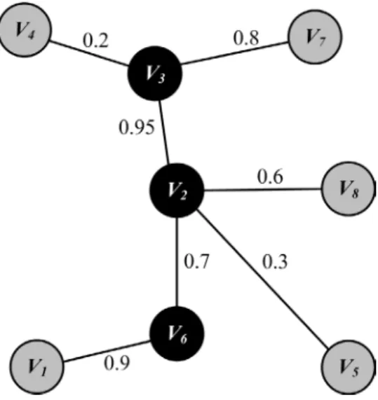
In this paper, our method is to construct the CDS by growing it from a single node outward. The single node is also referred to as the first dominator node. We choose the node which has the biggest EDDP as the first dominator. If there is more than one node with the biggest EDDP, we choose the node which has the big-gest delivery probability. The first dominator is colored black and all its uncolored neighbors are colored grey. According to Figure 2 and the EDDP in Section 3, we know the biggest EDDP of node 2 is 3, so node 2 is colored black, and its uncolored neighbors are colored grey.
After the first black node is determined, we judge whether the next node is a black node by using the highest delivery probability rank in all black nodes. If there is a node with the big-gest EDDP among all nodes directly connect-ing with the black nodes, but is not one of the black nodes, it is selected as the next domina-tor and colored black while all of its uncolored neighbors are colored grey. If such a node does not exist, then the delivery probability rank of the black nodes will be reduced by one level. The above procedure is repeated until the next dominator is selected out. According to Figure 3(a) and the EDDP calculated in Section 3, we know that the first black node is node 2, while
its delivery probability rank is 2. As node 3 has the highest link delivery probability between node 2 and its neighbors, which amounts to 0.95, additionally having the biggest EDDP ex-cept node 2, it is selected as the next dominator and colored black. Subsequently its uncolored neighbors are colored grey.
If one node and its neighbor nodes are colored grey or black, we also reduce the delivery ability rank in all black nodes' delivery prob-ability rank. Repeat the above steps until all nodes are black or grey. As shown in Figure 3(b), the black nodes are node 2 and 3. Node 7 has the highest link delivery probability among such probabilities between any black node and its neighbor nodes, i.e. 0.8; node 7 has also has the biggest EDDP except that of the black nodes. Hence, node 7 should have been selected as the next dominator but for the fact that it has already been colored, and is thus disqualified. Therefore, we try node 6 that has the second highest link delivery probability after node 7, namely 0.7. As node 6 is eligible, it is selected as the next dominator and colored black, af-ter which its uncolored neighbors are colored grey. At this point, all nodes are colored black or grey, and the construction of reliable CDS accomplished.
4.3. Allocation of Dominatees
After we have successfully constructed the re-liable CDS, the last step is the problem of the connection between dominatee and dominator. If a dominatee node has only one neighboring dominator node, then it delivers data to the dominator node; otherwise it delivers data to the dominator with the highest delivery probability among all its neighbor dominators. According to Figure 3(c) and the delivery probability rank table in Section 3, we know that node 4 just has one neighbor dominator, which is node 3, and node 8 has just one neighbor dominator, which is node 2, hence node 4 delivers data to node 3, while node 8 delivers data to node 2. Node 1 has more than one neighbor dominator, which are node 2 and node 6, node 5 has more than one neighbor dominator, which are node 2 and node 6, and node 7 has more than one neighbor dominator, which are node 2 and node 3. How-ever, the delivery probability between node 1 and node 6 is 0.9, which is the highest delivery
Algorithm 1. Effective degree of delivery ratio.
1. Initialization: flag(i) = 0; rank[i][ j] = 0; 2. for (i = 1; i <= N; i++)
3. for (j ≠ i; j <= N; j++)
4. Descending sort γij, rank[i][ j] = γij; 5. Calculate theγijof node i;
6. end for
7. Calculate theγijof all nodes;
8. end for
9. Delete rank[i][ j], if γij < γij; Figure 2. Node initialization. (a) Choose the first dominator.
(b) Node traverse.
(c) Breaking the tie.
The pseudo-code of selecting the delivery prob-ability threshold and the effective degree of de-livery probability are shown in Algorithm 1.
4. RVBP-CDS Algorithm
4.1. Node Initialization
According to the effective degree of delivery probability defined in Section 3, we know that there are some nodes whose EDDP is zero, and the delivery probability between these nodes and their neighbor nodes is lower than the de-livery probability threshold. The core idea of the algorithm is preferentially improving the reliability of dominators, that is to say, the de-livery probability between the dominator is the biggest. So, before we select the dominator node, the first step is removing the node whose degree is zero and identifying some domina-tees. We call this node initialization.
In this step, according to the EDDP, the node with zero degree is colored grey, other nodes are colored white. According to Figure 1 and the EDDP in Section 3, we know the EDDP about node 4 and node 5 is zero, so node 4 and node 5 are colored grey, other nodes are colored white in the initialization step.
4.2. Construction of a Reliable CDS
Connected dominating sets are one of the pri-mary techniques used to build virtual back-bones for wireless sensor and ad hoc networks. The concept of CDS can be briefly introduced as follows. A dominating set (DS) is a subset
of the vertices of a graph where every vertex in the graph is either in the subset or is adjacent to at least one vertex in the subset. A CDS is a connected DS. The nodes in CDS are called dominators, while other nodes are called dom-inatees [17].
In this paper, our method is to construct the CDS by growing it from a single node outward. The single node is also referred to as the first dominator node. We choose the node which has the biggest EDDP as the first dominator. If there is more than one node with the biggest EDDP, we choose the node which has the big-gest delivery probability. The first dominator is colored black and all its uncolored neighbors are colored grey. According to Figure 2 and the EDDP in Section 3, we know the biggest EDDP of node 2 is 3, so node 2 is colored black, and its uncolored neighbors are colored grey.
After the first black node is determined, we judge whether the next node is a black node by using the highest delivery probability rank in all black nodes. If there is a node with the big-gest EDDP among all nodes directly connect-ing with the black nodes, but is not one of the black nodes, it is selected as the next domina-tor and colored black while all of its uncolored neighbors are colored grey. If such a node does not exist, then the delivery probability rank of the black nodes will be reduced by one level. The above procedure is repeated until the next dominator is selected out. According to Figure 3(a) and the EDDP calculated in Section 3, we know that the first black node is node 2, while
its delivery probability rank is 2. As node 3 has the highest link delivery probability between node 2 and its neighbors, which amounts to 0.95, additionally having the biggest EDDP ex-cept node 2, it is selected as the next dominator and colored black. Subsequently its uncolored neighbors are colored grey.
If one node and its neighbor nodes are colored grey or black, we also reduce the delivery ability rank in all black nodes' delivery prob-ability rank. Repeat the above steps until all nodes are black or grey. As shown in Figure 3(b), the black nodes are node 2 and 3. Node 7 has the highest link delivery probability among such probabilities between any black node and its neighbor nodes, i.e. 0.8; node 7 has also has the biggest EDDP except that of the black nodes. Hence, node 7 should have been selected as the next dominator but for the fact that it has already been colored, and is thus disqualified. Therefore, we try node 6 that has the second highest link delivery probability after node 7, namely 0.7. As node 6 is eligible, it is selected as the next dominator and colored black, af-ter which its uncolored neighbors are colored grey. At this point, all nodes are colored black or grey, and the construction of reliable CDS accomplished.
4.3. Allocation of Dominatees
After we have successfully constructed the re-liable CDS, the last step is the problem of the connection between dominatee and dominator. If a dominatee node has only one neighboring dominator node, then it delivers data to the dominator node; otherwise it delivers data to the dominator with the highest delivery probability among all its neighbor dominators. According to Figure 3(c) and the delivery probability rank table in Section 3, we know that node 4 just has one neighbor dominator, which is node 3, and node 8 has just one neighbor dominator, which is node 2, hence node 4 delivers data to node 3, while node 8 delivers data to node 2. Node 1 has more than one neighbor dominator, which are node 2 and node 6, node 5 has more than one neighbor dominator, which are node 2 and node 6, and node 7 has more than one neighbor dominator, which are node 2 and node 3. How-ever, the delivery probability between node 1 and node 6 is 0.9, which is the highest delivery
Algorithm 1. Effective degree of delivery ratio.
1. Initialization: flag(i) = 0; rank[i][ j] = 0; 2. for (i = 1; i <= N; i++)
3. for (j ≠ i; j <= N; j++)
4. Descending sort γij, rank[i][ j] = γij; 5. Calculate theγijof node i;
6. end for
7. Calculate theγijof all nodes;
8. end for
9. Delete rank[i][ j], if γij < γij; Figure 2. Node initialization. (a) Choose the first dominator.
(b) Node traverse.
(c) Breaking the tie.
probability in node 1; the delivery probability between node 5 and node 2 is 0.3; which is the highest delivery probability in node 5, and the delivery probability between node 7 and node 3 is 0.8, which again is the highest delivery prob-ability in node 7. Hence, node 1 delivers data to node 6, node 5 delivers data to node 2, and node 7 delivers data to node 3.
The pseudocode of constructing the RVBP-CDS is shown in Algorithm 2.
5. Simulation Results
We compare our RVBP-CDS algorithm with the LBVBP-MOGA algorithm proposed in [10] and the RMCDS-GA algorithm proposed in [9] through the simulation experiment. We compare them in six main aspects: the network lifetime; the network delay; the packet delivery rate, the number of packet retransmissions, the average residual energy and the average dissi-pated energy. We compare the three algorithms in terms of network lifetime, which is defined as the time duration until the first dominator runs out of energy.
We build our own simulator where all the nodes have the same transmission range and all the nodes are deployed uniformly and randomly in a square area. For each specific setting, 100 instances are generated. Moreover, we assume that the node at the top end of the network is the the sink node, and data packets of all other nodes will be delivered to it. Furthermore, ev-ery sensor node produces a packet with size one during each communication interval. During the data transmission, we assume that the 1-hop transmission time is 0.1 s, if the data transmis-sion fails, and then continue retransmistransmis-sion of this package after 1 s. The simulated energy consumption model is that every node has the same initial 1000 units of energy. Receiving and transmitting a packet both consume 1 unit of energy. We assume that the communication interval changes from 3 s to 30 s and increases 3 s every time. The simulation parameters are listed in Table 1.
5.1. Network Lifetime
Figure 5 shows the network lifetime of three algorithms (RMCDS-GA, LBVBP-MOGA, RVBP-CDS) under the change of communi-cation interval. As we can see from the figure, the LBVBP-MOGA algorithm is better than the RMCDS-GA algorithm and our RVBP-CDS algorithm when the communication interval is less than 9 s. After more than 9 s, the RM-CDS-GA algorithm and our RVBP-CDS rithm are superior to the LBVBP-MOGA algo-rithm step by step. The cause for such behavior is that both algorithms – the RMCDS-GA and our RVBP-CDS – ensure the highest delivery probability between dominators, hence a packet generated by the source node can be delivered to the sink node in a short time. Thus the sink node shows apparent energy consumption, with a reduction of network lifetime. However, LB-VBP-MOGA has a low reliability in the nodes, i.e. a large number of data packets are blocked in the nodes with low delivery probability when the communication interval is relatively low; consequently the sink node has lower energy consumption, hence the respective network lifetime is longer than the one in our algorithm. In the RMCDS-GA algorithm, the reliable min-imum connected dominating set was used to construct the reliable virtual backbone, hence the respective network lifetime is longer than that of LBVBP-MOGA. But RMCDS-GA may create a situation in which the more domina-tees a dominator owns, the faster the energy of the dominator is consumed. The uneven energy
consumption of RMCDS-GA leads to a net-work lifetime which is shorter than that of our RVBP-CDS.
5.2. Network Delay
The network delay is defined as the average number which is computed by dividing the total delay by the number of all generated packets. Here, the total delay is the sum of the delays for transmission or retransmission of each packet. Figure 6 shows the network delay of three al-gorithms (RMCDS-GA, LBVBP-MOGA, RVBP-CDS) under the change of communi-cation interval. As we can see from the figure, the network delay of three algorithms reduces gradually. Finally, with the increase of commu-nication interval, the network delay of LBVB-P-MOGA algorithm is stable for about 13 s, and the RMCDS-GA algorithm and our RVBP-CDS algorithm are stable for about 1s. Analyzing the reason, the RMCDS-GA algorithm and our RVBP-CDS algorithm ensure the delivery probability between the nodes. Especially our RVBP-CDS algorithm, we preferentially con-sider the reliability of dominators, and then we improve the reliability between dominators and dominatees to the utmost extent. In this way, we can reduce the amount of data retransmission times, and then reduce the delay of the whole network. But the LBVBP-MOGA algorithm has a low reliability in nodes, which causes a lot of packet retransmissions, and then increase the delay of the whole network.
Figure 4. Allocation of dominatees.
Algorithm 2. RVBP-CDS.
1. for (i = 1; i <= N; i++) 2. if rank[i][ j] = 0, flag(i) = 2; 3. else degree[i] = j;
4. end for
5. if degree[i] is the MAX; 6. flag(i) = 1,all flag( j) = 2; 7. end if
8. if the MAXdegree[i] > 1, select the MAX γij, do 6; 9. for all nodes with flag = 1, select the MAX γij;
10. if degree[j] is the MAX except degree[i], 11. do 6,
12. end if; end for;
13. repeat 4,5 and 6, until all the node's flag = 1 or 2; 14. for all the nodes with flag = 2,
15. if they have one neighborhood with flag = 1, select it;
16. if they have more than one neighborhood with flag = 1, select the highest γij;
17. end if; end for;
Table 1. Simulation parameters.
Parameter Value
Node initial energy 1000 (unit)
Number of sensor 8
Node transmit energy 1 (unit/packet) Node receive energy 1 (unit/packet) 1-hop transmission time 0.1 (s) Retransmission time interval 1 (s)
Communication interval 3 ~ 30 (s) Packet numbers 1 (packet/interval)
3 6 9 12 15 18 21 24 27 30
500 1000 1500 2000 2500 3000 3500
Communication Interval(s)
Network Lifetime(s)
MCDS−GA LBVBP−MOGA RVBP−CDS
3 6 9 12 15 18 21 24 27 30
0 20 40 60 80 100 120
Communication Interval(s)
Network Delay(s)
MCDS−GA LBVBP−MOGA RVBP−CDS
5.3. Packet Delivery Rate
The packet delivery rate is calculated by di-viding the number of all generated packets by the number of all packets which arrived at the sink node. Figure 7 shows the packet delivery rate of three algorithms (RMCDS-GA, LBVB-P-MOGA, RVBP-CDS) under the change of communication interval. As we can see from the figure, the packet delivery rate of three al-gorithms increases gradually. Finally, with the increase of the communication interval, the packet delivery rate of LBVBP-MOGA sta-bilizes at around 0.85, while the ones of both RMCDS-GA and our RVBP-CDS at around 1.0. Analyzing the reason, the RMCDS-GA al-gorithm and our RVBP-CDS alal-gorithm ensure the delivery probability between the nodes, so packets can be transmitted to the sink node at a rapid rate, and the energy consumption in each node is also more balanced, so they have a higher packet delivery rate than the LBVB-P-MOGA algorithm. But the LBVBLBVB-P-MOGA algorithm has a low reliability between the nodes, which causes a lot of packet retransmis-sions, and this will run out of the dominator en-ergy with a lower probability, last it causes a fracture of the link and a large number of data packets can't be transmitted to the sink node.
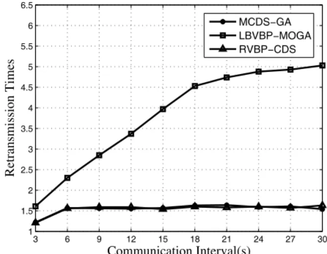
5.4. Retransmission Times
Retransmission times are calculated by dividing total retransmission times by the number of all generated packets. Here, the total
retransmis-sion time is the sum of retransmisretransmis-sion times for each packet. Figure 8 shows the retransmission times of three algorithms (RMCDS-GA, LB-VBP-MOGA, RVBP-CDS) under the change of communication interval. As we can see from the figure, the retransmission times of three al-gorithms increase gradually. Finally, with the increase of communication interval, the retrans-mission times of original LBVBP-MOGA algo-rithm is stability about 5, and the RMCDS-GA algorithm and our RVBP-CDS algorithm is sta-bility about 1. Analyzing the reason, the RM-CDS-GA algorithm and our RVBP-CDS algo-rithm ensure the delivery probability between the nodes, which greatly reduces the loss of data, thereby reducing the retransmission times. But the LBVBP-MOGA algorithm has a low reliability between the nodes, which increases the loss of data, and large amount of data pack-ets need to be retrainsmitted.
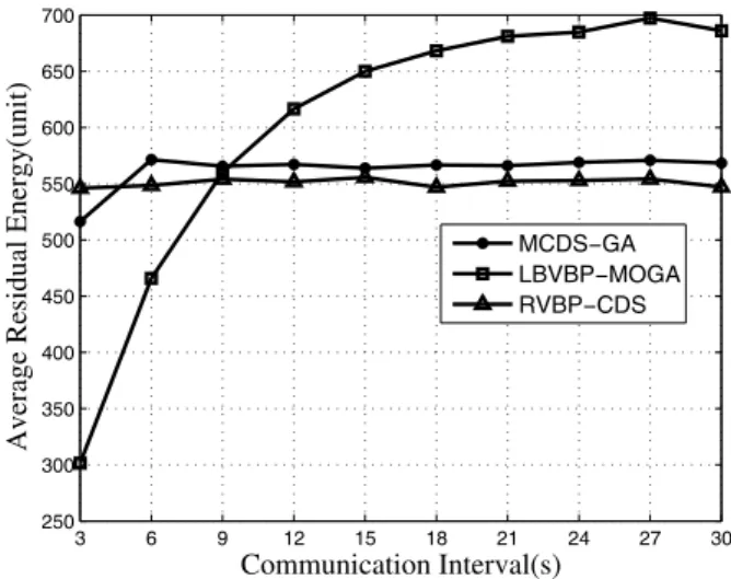
5.5. Average Residual Energy and Average Dissipated Energy
Average residual energy is calculated so that the total residual energy of all nodes is divided by the number of all nodes and average dissipated energy is calculated so that the total dissipated energy of all nodes is divided by the number of all nodes when the first dominator runs out of energy. Figure 9 and Figure 10 show the av-erage residual energy and avav-erage dissipated energy of three algorithms (RMCDS-GA, LB-VBP-MOGA, RVBP-CDS) under the change of
communication interval. As we can see from the figure, in both, the RMCDS-GA algorithm and our RVBP-CDS algorithm, average residual en-ergy and average dissipated enen-ergy are stable at a fixed value under the change of communica-tion interval, and the average residual energy of LBVBP-MOGA algorithm increases gradually. Finally, it is stability about 700, and the average dissipated energy of LBVBP-MOGA algorithm increases gradually, finally it is stability about 300 under the change of communication inter-val. Analyzing the reason, the RMCDS-GA al-gorithm and our RVBP-CDS alal-gorithm ensure the delivery probability between the nodes, re-duce the retransmission times, so they have a low dissipated energy and high residual energy.
6. Conclusion
In this paper, we address the topic of construct-ing a reliable virtual backbone in probabilistic wireless sensor networks. On the basis of re-moving the nodes with zero EDDP, we con-struct a reliable CDS through growing it from the node with the highest EDDP outward, step by step. And in the dominatee allocation, each dominatee selects the neighbor dominator node with the highest delivery probability to deliver data. The simulation results demonstrate that using a reliable CDS can significantly prolong the network lifetime. Specifically, our proposed algorithm prolongs the network lifetime by 118% to the maximum compared with the LB-VBP-MOGA algorithm and 20% to the max-imum, compared with the RMCDS-GA algo-rithm.
Acknowledgment
This work is supported by the National Natural Science Foundation of China under Grants No. 61662042, 61262081, and 61462056; the Yun-nan Provincial Key Project of Applied Basic Research Plan under Grants No. 2014FA028; the Fundamental Research Funds for the Central Universities under Grants No. ZYGX2012J083.
References
[1] S. Hadim and N. Mohamed, ''Middleware: Mid-dleware Challenges and Approaches for Wireless Sensor Networks'', IEEE Distributed Systems On-line, vol. 7, no. 3, pp. 1–1, 2006.
http://dx.doi.org/10.1109/MDSO.2006.19 [2] F. Ishmanov et al., ''Energy Consumption
Bal-ancing (ECB) Issues and Mechanisms in Wire-less Sensor Networks (WSNs): a Comprehensive Overview'', Eur. Trans. Telecomms, vol. 22, pp. 151‒167, Feb. 2011.
http://dx.doi.org/10.1002/ett.1466
[3] C. Schurgers and M. B. Srivastava, ''Energy Ef-ficient Routing in Wireless Sensor Networks'', in 2001 Military Communications Conference for Network-Centric Operations: Creating the Infor-mation Force, McLean, 2001, pp. 357‒361. http://dx.doi.org/10.1109/MILCOM.2001.985819 [4] X. Liang et al., ''Energy Efficient Modulation
Design for Wirless Sensor Networks'', in 2007 IEEE Pacific Rim Conference on
Communica-3 6 9 12 15 18 21 24 27 30
0.1 0.2 0.3 0.4 0.5 0.6 0.7 0.8 0.9 1
Communication Interval(s)
Packet Delivery Rate
MCDS−GA LBVBP−MOGA RVBP−CDS
Figure 7. Packet delivery rate.
3 6 9 12 15 18 21 24 27 30
1 1.5 2 2.5 3 3.5 4 4.5 5 5.5 6 6.5
Communication Interval(s)
Retransmission Times
MCDS−GA LBVBP−MOGA RVBP−CDS
Figure 8. Retransmission times.
3 6 9 12 15 18 21 24 27 30
250 300 350 400 450 500 550 600 650 700
Communication Interval(s)
Average Residual Energy(unit)
MCDS−GA LBVBP−MOGA RVBP−CDS
Figure 9. Average residual energy.
3 6 9 12 15 18 21 24 27 30
300 350 400 450 500 550 600 650 700
Communication Interval(s)
Average Dissipated Energy(unit)
MCDS−GA LBVBP−MOGA RVBP−CDS