Vol. 12, No. 4, 2019, 1567-1583 ISSN 1307-5543 – www.ejpam.com Published by New York Business Global
Identification of parameters of Richards equation using
Modified hybrid Grey Wolf Optimizer-Genetic
Algorithm (HmGWOGA)
Wenddabo Olivier Sawadogo1,∗, Pengdwend´e Ouss´eni Fabrice Ouedraogo2, Ouss´eni So3, G´en´evi`eve Barro4, Blaise Some5
1 University of Ouahigouya, Burkina Faso 2 University of D´edougou, Burkina Faso 3 Institute of Science, Burkina Faso 4 Ouaga 2 University, Burkina Faso
5 Joseph Ki Zerbo University, Burkina Faso
Abstract. In this paper, it is a question of identification of the parameters in the equation of Richards modelling the flow in unsaturated porous medium. The mixed formulation pressure head-moisture content has been used. The direct problem was solved using Multiquadratic Radial Basis Function ( RBF-MQ ) method which is a meshless method. The Newton-Raphson’s method was used to linearize the equation. The function cost used is built by using the infiltration. The optimization method used is a meta-heuristic called Modified hybrid Grey Wolf Optimizer -Genetic Algorithm (HmGWOGA). A test on experimental data has been carried. We compared the results with genetic algorithms. The results showed that this new method was better than genetic algorithms.
2010 Mathematics Subject Classifications: 65M06,76S05,74F10,90C59
Key Words and Phrases: Unsaturated porous medium, equation of Richards, RBF-MQ method, inverse problem, global optimization, meta-heuristic
1. Introduction
The fluid movement in unsaturated porous medium is governed by the Richards equa-tion [2, 24] which contains parameters that take into account type of the considered soil. The calculation of the water balance on a soil-scale requires knowledge of infiltration that is obtained by solving the unsaturated flow equation. However The hydrodynamic param-eters of the soils involved in the equation are, in most cases, badly known. The values ∗
Corresponding author.
DOI: https://doi.org/10.29020/nybg.ejpam.v12i4.3564
Email addresses: [email protected](W. O. Sawadogo),
[email protected] (P. O. F. Ou´edraogo),[email protected](O. So),
barro [email protected](G. Barro),[email protected](B. Som´e)
given in the literature are not precise values but intervals, hence the importance of the inverse modeling.
Estimating parameters in unsaturated porous environments is not trivial. Indeed, it re-quires numerical resolution of the Richards equation. The numerical methods used must allow a good estimate of hydraulic pressure and water content. Several methods have been proposed for solving the Richards equation: the finite difference method [2], the fi-nite volume method [1], the fifi-nite element method, the mixed fifi-nite element method [6]) and the discontinuous finite element [22]. Theses methods are based on the mesh of the domain in which the problem must be discretized. The mesh must obey certain rules. For example, the elements should not be overwritten to prevent the associated Jacobian from degenerating. This makes their implementation difficult and expensive ins some cases. To overcome these shortcomings, meshless methods called Radial basis function (RBF) have been developed since the 1970s. The idea is to reconstruct a function defined on a continuous space from the set of discrete values taken by this function on a not connected point cloud of the physical domain. Stevens and Power [23] used a implicit RBF method to solve the pressureh formulation of Richards equation. More recently, F. Motaman and al. [16] used the RBF-DQ method to solve the moisture contentθformulation. These two formulations have limits. In this work, we use the RBF-MQ method to solve the mixed formulation of Richards equation.
There exist many methods to solve the inverse problems [4, 12, 13, 19]. Most computing software in hydrogeology use deterministic methods. However most of these methods re-quire a good knowledge of the solution. Indeed, these algorithms can not detect a global optimum and can stop with a local optimum. Moreover, these algorithms require a certain regularity of the functions to be optimized. However, this regularity is not always checked. Meta-heuristic optimization techniques are adapted better to the problems of optimization in which the size of the space of research is important, where the parameters interact in a complex way and where very little information on the function to be optimized is available [7, 15]. The function to be optimized can thus be the result of a simulation. These algo-rithms are often much more robust in their capacity to identify the total optimum with less sensitivity to the initial condition.
2. Direct problem
2.1. Mathematical model
There exist several formulations of the equation of Richards which models the flow in unsaturated porous medium but in this work, we use the mixed formulation pressure head-moisture content because the numerical solutions obtained with his mixed formulation are more precise [2, 14].
In one dimension, the mixed formulation is given by :
∂θ(h)
∂t +
∂
∂zq(h) =f in Ω×[0, T]
q(h) =−K(h)∂z∂h−K(h) in Ω×[0, T]
h=hinit in Ω
h=gD on∂ΩD×[0, T]
q(h) =gN on∂ΩN×[0, T]
(1)
with :
• Ω = [a, b]⊂R represents a column of water infiltration;
• z denotes the vertical dimension:
• h[L] the pressure head;
• gD and gN are respectively imposed pressure and flow on the boundaries ∂ΩD and
∂ΩN;
• q(h) the flow velocity;
• hinit is the initial pressure head and f is a source function;
• θ[L3/L3] the moisture content given by: θ(h) = θs−θr
(1 + (α|h|)n)m +θr (2)
whereθr the moisture content to saturation (L3.L−3),θs the residual moisture
con-tent (L3.L−3), α a parameter of form related to the mean size of the pores (L−1), n a parameter related to the distribution of the sizes of pores (−). According to Mualem [17], we havem= 1−1/n.
• K(h) is the insaturated hydraulic conductivity [L/T]. We use the relation of Van Genuchten [24] given by
K(Se) =KsSe1/2(1−(1−Se1/m)m)2 (3)
withKS the effective saturated hydraulic conductivity [L/T].
Se the effective saturation given by:
Se =
θ−θr
θs−θr si h <0
h and θare related by the moisture capacity function C(h)[1/L] defined by
C(h) = ∂θ
∂h (5)
Whats gives
C(h) =−αn(θr−θs)sign(h)(
1
n−1)(α|h|)
n−1(1 + (α|h|)n)1/n−2 (6)
To solve the problem (1), you need to know the parameters α,θS,θr,nand KS.
2.2. Numerical resolution of direct problem
2.2.1. Description of RBF-MQ method
Appeared in the 1970s [3], it was Kansa who introduced the PDE resolution using the Radial Basis Funtions (RBF) method [10, 11].
We consider a numerical function u(x), x ∈ Rd where d is the space dimension. The MQ-RBF method consist to approximate u by
ˆ u(x) =
M
X
j=1
λjφ(kx−xjk, c), x∈Rd (7)
where
xj, j = 1, . . . , M are thecenters of the RBF approximation
φthe basic radial function of Hardy [8] given by φ(r, c) =√r2+c2 c the precision parameter.
Expansion coefficients λj, j = 1, . . . , M are determined by setting: M
X
j=1
λjφ(kxi−xjk, c) =u(xi), i= 1, . . . , M
Which is expressed in the following matrix form:
Aλ=U (8)
where
λ= (λ1, λ2, . . . , λM)>, U = (u(x1), u(x2), . . . , u(xM))>
and
A=
φ(kx1−x1k, c) φ(kx1−x2k, c) . . . φ(kx1−xMk, c)
φ(kx2−x1k, c) φ(kx2−x2k, c) . . . φ(kx2−xMk, c)
..
. ... . .. ...
..
. ... . .. ...
φ(kxM −x1k, c) φ(kxM −x2k, c) . . . φ(kxM −xMk, c)
According to [9]λis given by
λ=A−1U (9)
The korder derivative of ˆuat the center xi is:
∂kuˆ(xi)
∂xk = M
X
j=1
λj
∂k
∂xkφ(kxi−xjk, c), i= 1,2, . . . , M (10)
In matrix form , the derivative (10) is written as :
U(k)=A(k)λ (11)
with
U(k)=
∂kuˆ(x1) ∂xk ,
∂kuˆ(x2) ∂xk , . . . ,
∂kuˆ(xM)
∂xk
and
A(k)=
∂k
∂xkφ(kx1−x1k, c) ∂
k
∂xkφ(kx1−x2k, c) . . . ∂
k
∂xkφ(kx1−xMk, c)
∂k
∂xkφ(kx2−x1k, c) ∂
k
∂xkφ(kx2−x2k, c) . . . ∂
k
∂xkφ(kx2−xMk, c)
. . . ... . .. ... . . . ... . .. ... ∂k
∂xkφ(kxM−x1k, c) ∂
k
∂xkφ(kxM−x2k, c) . . . ∂
k
∂xkφ(kxM−xMk, c)
(12)
Using the expression of λ, we get:
U(k) =D(k)U (13)
where
D(k)=A(k)A−1 (14)
2.2.2. Space approximation of the Richards equation by the RBF-MQ method In this section, we present the numerical resolution of problem (1). This approach was proposed by Ou´edraogo et al. [18].
Let {zi}16i6M a set of points of Ω considered as centers. At each center zi the
approxi-mation value ˆh of the pressure headh by the RBF-MQ is given by:
ˆ
h(zi, t) = M
X
j=1
λj(t)φ(kzi−zjk, c), t∈]0, T] (15)
whereφ the basic radial function of Hardy. that can be rewritten in matrix form
whereh= (h(z1, t), h(z2, t), . . . , h(zM, t))> and λ(t) = (λ1(t), λ2(t), . . . , λM(t))>.
the flow velocity q(h) is given by
q◦ˆh(zi, t) = M
X
j=1
γj(t)φ(kzi−zjk, c), t∈]0, T], zi, i= 1,2, . . . , M
Whereγj(t), j = 1,2, . . . , M the expansion coefficients of q(h).
In matrix form, we have
q(h) =A Γ(t), t∈]0, T] (17)
where Γ(t) = (γ1(t), γ2(t), . . . , γM(t))>.
Using expression of ˆh we have
q(h, t) =−KD(h, t)D(1)h(t)−K(h, t), t∈]0, T] (18)
where
K(h) = (K◦h1, K◦h2, , . . . , K◦hM,)>
et
KD(h) =
K◦h1
K◦h2 0 0 . ..
K◦hM
withhi=h(zi, t), i= 1, . . . , M, t∈]0, T] theith value of the vectorh (16).
using 11, we have ∂
∂zq(h)'q
(1)(h) =−D(1)K
D(h)D(1)h−D(1)K(h) (19)
Let Θ(h) = (θ◦h1, θ◦h2, , . . . , θ◦hM)> and f = (f(z1, t), f(z2, t), . . . , f(zM, t) be the
values respectively of the moisture content θ(h) and the source function f at the centers zi, i= 1,2, . . . , M.
The numerical resolution of Richards’ equation (1) can then resume to the resolution of the following problem in time:
(dΘ(h)
dt =F(h), t∈]0, T]
h(0) =h0
(20)
with
F(h) =q(1)(h) +f (21)
and
2.2.3. Resolution by Newton-Raphon’s method
Let tn = nδt, n = 0,1, . . . , N a discretization of [0, T], δt = T /(N −1) the time-step
size and Θn, Fn the approximations of Θ(hn, t
n) and F(hn, tn) with hn = h(tn), n =
0,1, . . . , N.
The approximation of the equation (20) by a implicit Euler scheme gives Θn+1−Θn
δt =F
n+1, n= 0,1, . . . , N−1 (22)
The terms Θn+1 and Fn+1 cause equation (22) to be highly nonlinear, we use Newton-Raphson’s method to solve it.
Let’s denote Θn+1,m+1,Kn+1,m+1
D andKn+1,m+1the approximated values Θ(hn+1,m+1),KD(hn+1,m+1)
and K(hn+1,m+1) in which hn+1,m+1 is the searched value of hn+1 in the step m+ 1 of Newton’s iterative process. Let’s also denote hn+1,m the value of hn+1 at the previous step m,
F(hn+1,m,hn+1,m+1) =−D(1)KDn+1,mD(1)hn+1,m+1−D(1)Kn+1,m+fn+1 (23) and
R(hn+1,m,hn+1,m+1) = Θ
n+1,m+1−Θn
δt − F(h
n+1,m,hn+1,m+1) (24)
Using a one-order Taylor’s series development of Θn+1,m+1, we obtain the following ap-proximation
Θn+1,m+1 'Θn+1,m+dΘ
n+1,m
dh δh
n+1 (25)
where
δhn+1=hn+1,m+1−hn+1,m (26) We denoteCn+1,m the value ofCin the approximated vectorhn+1,mthen the approx-imation (25) can be rewritten as following:
Θn+1,m+1 'Θn+1,m+Cn+1,mδhn+1 (27) We then replace Θn+1,m+1 in equation (25) by its expression given by (27) and therefore we obtain the new expression ofR(hn+1,m,hn+1,m+1) as following:
R(hn+1,m,hn+1,m+1) = 1 δtC
n+1,mδhn+1+ Θn+1,m−Θn
δt − F(h
n+1,m,hn+1,m+1) (28)
The resolution of nonlinear problem (22) with the Newton-Raphson’s iterative method consists in solving at each time-stepn+ 1 and at each stagem+ 1, the equation
whereJ is Jacobian matrix of Rin hn+1,m expressed as J = dR
dh(h
n+1,m,hn+1,m) = 1
δtC
n+1,m−D(1)K
D(hn+1,m)D(1) (30)
until kδhn+1k is below a certain tolerance tol or that m exceeds a maximum value maxiter. Algorithm 1 describes how the Richards equation is solved at each time-step n+ 1 by Newton’s iterative method.
Algorithm 1 Newton-Raphson’s iterative method
Require: hn, maxiter, tol hn+1,0 =hn
while m6maxiter andkδhn+1k> tol do Solve the system (29) to obtainδhn+1 hn+1,m+1=hn+1,m+δhn+1
m=m+ 1 end while hn+1=hn+1,m+1 Ensure: hn+1
3. Inverse problem
3.1. Calculation of infiltration
One of the objectives of the modeling of the flow in unsaturated porous medium is the estimate of the quantity of water which infiltrates to reach the saturated zone. The infiltration describes the process of water penetrating in the ground starting from its surface. In a general way, for a variable initial conditionθ(0, z), the cumulative infiltration Icum is defined by:
Icum(t) =
Z Z
0
q(t, z)dz
q(z, t) is the rate of infiltration andZ is the depth of the ground considered. If the initial condition θinit is constant, we have:
Icum(t) =
Z Z
0
(θ(t, z)−θini)dz (31)
θ(t, z) is the moisture content. In discrete formIcum(tj) is obtained by making an
approx-imation of (31) by the formula of the trapezoids:
Icum(tj) = ∆z
"
1
2(θsup−2θini+θinf) +
Nz
X
i=1
θji −θini
#
(32)
3.2. Function cost
Let thus M observations of values of infiltration Iobs(tj) at the moments tj, j =
1, . . . , M. Let thusJ the functional defined by
J(U) = ∆t 2
M
X
j=1
(Icum(tj)−Iobs(tj))2
= ∆t 2
2
X
j=1
(∆z
"
1
2(θsup−2θini+θinf) +
Nz
X
i=1
(θij−θini)
#
−Iobs(tj))2 (33)
U is the vector of parameters to determinate (α, n, θr, θs, Ks).
The inverse problem consists in solving min
U⊂DJ(U) (34)
whereD a bounded subset ofR5.
4. Problem solving by Modified hybrid Grey Wolf Optimizer-Genetic Algorithm (HmGWOGA)
In this section we present the HmGWOGA algorithm proposed by Sawadogo et al. [20]. This algorithm is a hybridization of two meta heuristics. Grey Wolf Optimizer algorithm proposed by S. Mirjalili et al. [15], and a version of genetic algorithm proposed by Sawadogo et al. [21].
We consider the following problem:
min
x∈Df(x) (35)
where x = (x1,· · ·, xn) ∈ Rn, f a positive numeric function of Rn, D = Qni=1[ai, bi], ai
and bi are reals.
4.1. Presentation of the genetic algorithm used
The genetic algorithm used is an adaptation of Non-Dominated Sorting Genetic Algorithm-II (NSGA-Algorithm-II) proposed by Deb et al. [5].
This algorithm consist to create at each iteration t a population of children (Qt) of size
(N) by using selection, crossing, and mutation operators. This population is add to a population of parents (Pt) of size (N) to form a population (Rt=Pt∪Qt). This process
variablexi of fitnessfi (evaluation of the function inxi) reintroduced in a new population
of size N is:
p= PNfi
j=1fj
The barycentric crossing is used but we did not use a probability of crossing. Mutation of a Gaussian type is applied to the population. One selects an individual x under a probabilityp. Ifpis lower than the probability of mutationpm, one adds a Gaussian noise
tox.
4.2. Grey Wolf Optimizer algorithm description
The GWO algorithm is a meta-heuristic which mimics the leadership hierarchy and hunting mechanism of grey wolves in nature. This algorithm has been proposed by S. Mirjalili et al [15]. Four types of grey wolves are employed for the simulating the leadership hierarchy: alpha (α), beta (β), (δ) and omega (ω).
Alpha is the leader of the group. Beta is the second. They help the alpha make decision. Delta are is the third category. Its members are scouts, sentinels and hunters. Last category omega wolves always have to submit to all the other dominant wolves.
Prey encircling is modeled by:
(
~
D=|C. ~~ Xp(t)−X~(t)|
~
X(t+ 1) =X~p(t)−A. ~~ D
(36)
where t indicates the current iteration, A~ = 2a. ~r1, C~ = 2. ~r1; ~a are decreased from 2 to 0 over the course of iterations and r1~, r2~ are random vectors in [0,1]. X~p is the position
vector of the prey, and X~ indicates the position vector of a grey wolf.
For better exploration of candidate solutions which tend to diverge when |A~|>1 and to converge when |A~|<1.
Grey wolves have the ability to recognize the location of prey and encircle them. Over the course of iterations, the first three fittest solutions we obtain so far are considered asα,β andδ respectively, which guide the optimization processes (the hunting) and are assumed to take the position of the optimum (the prey). The approximate distance between the current solution and alpha, beta and delta is given by the following formula:
~
Dα=|C1. ~~ Xα−X~|
~
Dβ =|C~2. ~Xβ −X~|
~
Dδ=|C3. ~~ Xδ−X~|
(37)
where:
• C~1,C~2 and C~3 are random vectors.
• X~α,X~α and X~δ, the positions of alpha, beta and delta respectively.
Finally the next position of the solution is given by: ~
X(t+ 1) = 0.7×X1~ + 0.2×X2~ + 0.1×X3~ (38) where
~
X1 =X~α−A~1. ~Dα
~
X2 =X~β −A2. ~~ Dβ
~
X3 =X~δ−A~3. ~Dδ
(39)
~
A1,A~2 and A~3 are random vectors.
4.3. Problem solving algorithm
Algorithm 2 Problem solving algorithm
Initialize the input parameters for HmGWOGA (N, d, lb, ub, M axiter, pm, sigma)
Initialize Alpha, Beta and Delta Position and Score. Initialize the random position of search agents. k←0
while k < M axiter do solving direct problem (1)
evaluate the score of each search agent (Pk) using objective function (33)
Apply a selection operator
Apply a crossover operator to generate a new population of child Qk (The criterion
used at this step is 1/(f itness+) with (∈R∗+)
Rk=Pk∪Qk (addQk toPk) to obtain 2N search agents
foreach agent inRk do
choose a random numberu in [0,1] if u≤pm then
Apply a mutation operator end if
end for
Classify search agents ofRkfrom increasing order according to the score of each agent
Keep N best individuals ofRk to form a new search agent.
fori i=1 to N do
f itness←− Score agent i if f itness < AlphaScore then
Update alpha end if
if f itness > AlphaScore and f itness < BetaScorethen Update beta
end if
if f itness > AlphaScore and f itness > BetaScore and f itness < DeltaScore then
Update delta end if
end for
fori=1 to N do
Update the Position of search agents including omegas using equation (37-39) Update the position of prey using equation(38)
end for k←k+ 1 end while
5. Results and discussions
5.1. Application 1
Either an unsaturated medium represented by a domain Ω = [0,20] and a simulation time interval [0,600]. Dirichlet conditions were imposed. According to [22], an analytical solution of the problem (1) is given by:
h(z, t) = 20.4 tanh(0.5(z+t/12−15))−41.5 (40) The source term f is chosen using the analytical solution.
To verify the efficiency of our algorithm data was generated using the analytical solu-tion.
The simulation conditions and the results are given below:
Parameters Range used values identified values
θs [0; 4] 0.357 0.364
θr [0; 4] 0.108 0.106
α [0; 1] 0.0335 0.032
n [0; 10] 1.8 1.87
Ks [0; 15]×10−3 8.13×10⁻³ 8.25×10⁻³
Value of objective function: 7.5×10⁻⁵.
Figure 1 shows the infiltration curve. In this figure we see that the identified infiltration is very close to the infiltration obtained with the analytical solution.
time
0 100 200 300 400 500 600
infiltration
0 0.5 1 1.5 2 2.5 3
Simulated Observed
5.2. Application 2
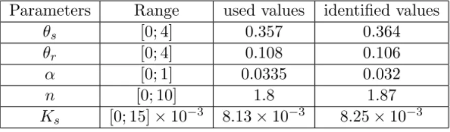
In this second application, we use data used in [21]. These were measured on a clay soil on a column of 1mlong. The values of the infiltration were recorded all the 5 mn during 2 hours. [21] In the direct problem was resolution using the finite difference method and the genetic algorithm was used to identify the parameters. The results of the identification are given in the table below
Parameters Interval Genetic algorithm HmGWOGA algorithm
θs [0; 1] 0.0238 0.0255
θr [0; 2] 0.379 0.373
α [0; 1] 0.0879 0.0869
n [0; 3] 1.1359 1.1395
Ks [0; 3]×10−5 1.75×10⁻⁵ 1.84×10⁻⁵
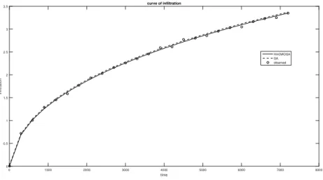
Figure 2 is a comparative representation of the simulated and observed infiltration curves. In these figures, we can see the quality of the estimation of the parameters. We also see that the curve obtained by HmGWOGA method is closer to the observed data than that obtained by GA. Which is confirmed by the values of the function cost:
Genetic algorithm: 0.0027 [21]. HmGWOGA algorithm:0.00012.
time
0 1000 2000 3000 4000 5000 6000 7000 8000
infiltration
0 0.5 1 1.5 2 2.5 3 3.5
curve of infiltration
HmGWOGA GA observed
Figure 2: Application2: Curves of infiltration observed and simulated
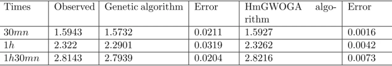
Times Observed Genetic algorithm Error HmGWOGA algo-rithm
Error
30mn 1.5943 1.5732 0.0211 1.5927 0.0016
1h 2.322 2.2901 0.0319 2.3262 0.0042
1h30mn 2.8143 2.7939 0.0204 2.8216 0.0073
Table 1: Comparison to test points
Figure 3: Application 2:Curves of convergence
To measure the performance of both methods in terms of computation time, we ran the simulation 30 times for each example. The characteristics of the computer used are: Processor: Intel(R)Xeon (R) CPU E5-2603 [email protected] GHz 1.7GHz, RAM: 24 GB, Operating System: windows 10, 64-bit.
The statistical results in second are given in the table 2.
HmGWOGA GA
Min Max Mean Std Min Max Mean Std
Application 2
608.125 609.468 608.757 1.481 421.23 422.39 426.787 1.67
Table 2: Computation time
These results show that although HmGWOGA is more accurate, it is slower than GA.
6. Conclusion
which is a meshless method. We used Modified Grey Wolf Optimizer-Genetic Algorithm (HmGWOGA) to determine parameters of Richards equation using synthetic data and real data. Comparison with the genetic algorithm showed that the HmGWOGA algo-rithm was more effective in identifying parameters involved in the Richards equation. A comparison of the execution times of the two algorithms shows the HmGWOGA algo-rithm despite its effectiveness remains slower than GA. In order to reduce execution time, we intend in the future to propose a parallel version of this algorithm.
References
[1] V. Baron, Y. Coudi`ere, and P. Sochala. Comparison of DDFV and DG methods for flow in anisotropic heterogeneous porous media. Gas Science and Technology–Revue d’IFP Energies nouvelles, 69:673–686, 2014.
[2] M. A. Celia and E. T. Bouloutas. A general mass-conservative numerical solution for unsaturated flow equation. Water Resources Rechearch, 26(7):1483–1496, 1990. [3] W. Chen, Z.J Fu, and C.S. Chen. Recent advances in radial basis function collocation
methods . Springer, 2014.
[4] Archa Rowan B. Cockett. A framework for geophysical inversions with application to vadose zone parameter estimation. PhD thesis, University of British Columbia, 2017. [5] Kalyanmoy Deb, Amrit Pratap, Sameer Agarwal, and T. Meyarivan. A Fast Elitist Multiobjective Genetic Algorithm: NSGA-II . IEEE Transactions on Evolutionary Computation, 6(2):182–197, 2002.
[6] M.W. Farthing, C. E. Kees, and C. T. Miller. Mixed finite element methods and higher order temporal approximations for variably saturated groundwater flow . Ad-vances in Water Resources, 26:373–394, 2003.
[7] D.E. Goldberg. Genetic Algorithms in Search, Optimization and Machine Learning.
MA Addison Wesley, 1986.
[8] R.L. Hardy. Multiquadric equations of topography and other irregular surfaces .
Journal of geophysical research, 76:1905–1915, 1971.
[9] R.L. Hardy and M.D. Buhmann. Radial basis functions: theory and implementations . Cambridge university press, 2003.
[10] E.J. Kansa. Multiquadrics – A scattered data approximation scheme with applications to computational fluid-dynamics – I surface approximations and partial derivative estimates . Computers & Mathematics with applications, 19:127–145, 1990.
partial differential equations . Computers & mathematics with applications, 19:147– 161, 1990.
[12] M. Kern. M´ethodes num´eriques pour les probl`emes inverses . ISTE Editions, 2016. [13] D. McLaughlin and L. R. Townley. A reassessment of the groundwater inverse problem
. Water Resources Research, 22(5), 1996.
[14] P.C.D. Milly. A mass-conservative procedure for time-stepping in models of unsatu-rated flow . Advance in Water Ressources, 8:32–36, 1985.
[15] Seyedali Mirjalili, Seyed Mohammad Mirjalili, and Andrew Lewis. Grey Wolf Opti-mizer . Advances in Engineering Software, 69:46–61, 2014.
[16] F. Motaman, G.R. Rakhshandehroo, M.R. Hashemi, and M. Niazkar. Application of RBF-DQ Method to Time-Dependent Analysis of Unsaturated Seepage .
[17] Y. Mualem. A new model for predicting the hydraulic conductivity of unsaturated porous media. Water Resources Research, 12:513–522, 1976.
[18] P. O. Fabrice Ou´edraogo, W. Olivier Sawadogo, and Ouss´eni So. Numerical resolution of Richards equation by the RBF-MQ method . Annals of the University of Craiova, Mathematics and Computer Science Series, 46(1):109–124, 2019.
[19] Gwladys Ravon. Probl`emes inverses pour la cartographie optique cardiaque. PhD thesis, Universit´e de Bordeaux, 2015.
[20] W. O. Sawadogo, P. O. F. Ou´edraogo, K. Som´e, N. Alaa, and B. Som´e. Modified hybrid Grey Wolf Optimizer and Genetic Algorithm (HmGWOGA) for global op-timization of positive functions . Advances in Differential Equations and Control Processes, 20(2):187–206, 2019.
[21] Wenddabo Olivier Sawadogo, Noureddine Alaa, Youssouf Par´e, and Blaise Som´e. Identification of the parameters of the equatioof Richards by the genetic algorithms . Advances in Theoretical and Applied Mathematics, 11(1):17–28, 2016.
[22] Pierre Sochala. M´ethodes num´eriques pour les ´ecoulements souterrains et couplage avec le ruissellement. PhD thesis, Paris Est, 2008.
[23] D. Stevens and H. Power. A scalable and implicit meshless RBF method for the 3D unsteady nonlinear Richards equation with single and multi-zone domains . Int. J. Numer. Methods Eng., 85:135–163, 2011.