Multi-class Image Classification Based on Fast Stochastic Gradient Boosting

(1)

Multi-class Image Classification Based on Fast Stochastic Gradient Boosting

Lin Li1,2, Yue Wu1and Mao Ye1

1_{School. of Computer Science and Engineering, University of Electronic Science and Technology of China}

No.2006, Xiyuan Ave, West Hi-Tech Zone, Chengdu, China E-mail: [email protected]

2_{Sichuan TOP IT Vocational Institute No.2000, Xixin Ave, West Hi-Tech Zone, Chengdu, China}

Keywords:multi-class image classification, fast random gradient boosting, multi-class classifier, machine learning, image data set

Received:December 3, 2013

Nowadays, image classification is one of the hottest and most difficult research domains. It involves two aspects of problem. One is image feature representation and coding, the other is the usage of classifier. For better accuracy and running efficiency of high dimension characteristics circumstance in image classifica-tion, this paper proposes a novel framework for multi-class image classification based on fast stochastic gradient boosting. We produce the image feature representation by extracting PHOW descriptor of im-age, then map the descriptor though additive kernels, finally classify image though fast stochastic gradient boosting. In order to further boost the running efficiency, We propose method of local parallelism and an error control mechanism for simplifying the iterating process. Experiments are tested on two data sets: Optdigits, 15-Scenes. The experiments compare decision tree, random forest, extremely random trees, stochastic gradient boosting and its fast versions. The experiment justifies that (1) stochastic gradient boosting and its extensions are apparent superior to other algorithms on overall accuracy; (2) our fast stochastic gradient boosting algorithm greatly saves time while keeping high overall accuracy.

Povzetek: Predstavljena je primerjava algoritmov za veˇcrazredno klasifikacijo slik.

1 Introduction

With the extensive application of the Internet, search en-gines have become an important tool for people to obtain information, including image information which is one of the most important and interesting information. Traditional search engines on the Internet, including Google, Bing and Baidu have launched a corresponding image search func-tion, but this kind of searching is mainly operated by the file names or related text information of the images. However, it has obvious limitations such as: file name or related in-formation is not accurately related with the image content. So information retrieval based on image content becomes one of the hottest studies of the image retrieval. image clas-sification is based on the image content-based information retrieval, which is based on visual information. Image clas-sification mainly involves two aspects: One is the image feature representation and coding, on the other hand is a classifier selection.

Haralick etc. [1] first proposed a method for feature representation based on image texture features, which is considering the texture characteristics of the image feature space relations, texture and spectral information and its sta-tistical characteristics. Later, considering rotation, affine and other factors, people gradually propose feature rep-resentation methods such as LBP [2], SIFT [3], HOG[4]

and etc. Statistical represented feature coding method has been widely used, for example a typical representative of

the texture histogram representation (histogram of textons)

[5]and bag of words or bag of features[6]coding. In recent years, people also proposed a histogram-based pyramid en-coding as PHOG (Pyramid Histogram Of Gradient)[7]and PHOW (Pyramid Histogram Of visual Word)[8]. In order to further improving the discriminative capability of feature descriptors, people propose kernel transformation such as Vedaldi’s additive kernel transformation[9]can effectively enhance classification performance.

(2)

2 Fast stochastic gradient boosting

algorithm

2.1 Analysis and comparison of algorithms

based on decision tree

Traditional classification and regression trees (Classifica-tion and Regression Tree, CART) proposed by Breiman

[15]is a simple and effective method, but there are many flaws[16]: 1) because decision tree is based on local opti-mum principle, this will led to the whole tree is not often global optimal. 2) inaccuracies and abnormal training sam-ples have a great impact on the CART. 3) The imbalances of training sample types also affect CART performance.

Improving and enhancing the performance of classifica-tion and regression trees is a valuable quesclassifica-tion. In recent years, bagging and boosting method is the most effective ways. Bagging method [17]is an autonomous improving method, which is a random subtree building based on sub-sampling over all training samples to obtain samples.

Bagging method proposed by the Breiman [18] is also based on random forest, which use decision trees as a meta-classifier with independent clustering method (Bootstrap aggregation, Bagging), thus produces different training set to generate each component classifier, and finally deter-mine the final classification results by a simple majority vote.

Extreme random tree[19]is similar to the random for-est. The tree pieces are combined to form a multi-classifier, the difference with the random forest mainly involving two sides:

1) Sampling the original training samples with replace-ment strategy, aiming at reducing bias;

2) Splitting test threshold of each decision tree node is selected at random. Assuming split test expression is

split(x) > θ, wherexis to be classified samples,splitis the test function in the random forest classifier, θ is usu-ally based on a sample of a feature set, and in the extreme random forest classifier,θis randomly selected.

Boosting method [20] is the method, which is starting from the basic classification tree, though iterative process, wrong classification of data give higher weights to build a new round of classification trees greater emphasising on these error detection data. Final classifier classification is based on the principle of majority voting. Despite boost-ing method is not accurate in some particular cases. But in most cases, it significantly enhances the classification ac-curacy[21].

ated from residual losses of the gradient direction of the model in order to reduce losses. Inspiring by bagging ran-dom thoughts of Breiman, Friedman introduced stochastic gradient boosting based on random sub-sampling to obtain training samples[23].

In short, bagging and boosting methods both can be called to vote or integrated approach to generate a set of sub-tree or forests, while classification is according to the sub-tree or forest in the whole set or voting on every tree. The difference is that they generate different sub-tree or forests by different ways.

2.2 Fast stochastic gradient boosting

algorithm

Fast stochastic gradient boosting algorithm is shown in the Algorithm 1. whereπ(i)N

1 is the random combinations of set of integers1,2, ..., N, assuming sample size of random down-sampling isN < Nˆ , The corresponding sample re-sult is(yπ(i), xπ(i))

ˆ

N

1. Fm(x)is for the firstmpoints. L

is the loss function,M is the number of weak classifiers,

Cis class sample,Ris the leaf node region,J is a termi-nal leaf number of nodes,ρis the optimal weak classifier coefficient,Sis the number of samples to detect the error,

erranderrminare the exit variable,parallelrefers

paral-lel processing.

Algorithm inputs are training samples, outputsF˜(x)are the output set of weak classifiers.

The step 1 to 17 of the algorithm is weak classifier train-ing processes consisttrain-ing of three components: The step 2 is randomized sampling. The steps 3 to 10 is weak classifier training stages. The step 11 to 16 is error detection.

The step 2 obtains training samples by randomly sam-pling for each weak classifier. The step 3 to 10 is weak clas-sifiers training process by classes in turn, which contains: 1) calculating the loss, the loss for classification problems using deviance loss; 2) by calculating the value of the loss of function in the negative gradient of the current model, which was estimated as a residual;3) training a decision tree classifier based on the basic decision tree;4) updating resid-uals;5) calculating the optimal weak classifier coefficients; 6) generating a new weak classifiers.

The step 11 to 16 is error detection. Classification train-ing and each error detection are simultaneously. Weak clas-sifiers stop training when the error is less than a certain threshold.

(3)

Algorithm 1Fast stochastic gradient boosting algorithm.

Input:

training data set :T = (x1, y1),(x2, y2), ...,(xN, yN), xi∈RN, y∈Y ∈R, Nis the number of training samples.

initialization :F0(x) = 0, M = 100, err= 0, errmin= 0.0001.

Output:

combination set of classification trees :Fˆ(x)

.

1: form= 1toM do

2: random sampling of (parallel):π(m)ˆ(N)1 ₌_rand_{_}_perm₍_m₎N

1

3: fork= 0toCdo

4: calculating loss :pk(x) = exp(Fk(x))/P C

l=1exp(Fl(x)), k= 1,2, ..., C

5: calculating the gradient (parallel):

˜

yπ(i)k =−

"

∂L(

yπ(i)l, Fl(xπ(i))

C l=1)

∂Fkxπ(i)

#

{Fl(x)=Fl,m−1(x)}Y1

=yπ(i)k−pk,m−1(xπ(i)), i= 1,2, ...,N˜

6: basic training for weak classifiers (parallel): Based on the decision tree (CART).

7: calculating residuals (parallel):{Rjkm} J

j=1=J−terminal_node_tree(

˜

yπ(i)k, xπ(i) ˜

N

1)

8: calculating the optimal weak classifier coefficients :

ρjkm= arg min

C−1

C

P

xπ(i)∈Rjkmy˜π(i)k

P

xπ(i)∈Rjkm

y˜π(i)k

(1−

y˜π(i)k

)

, j= 1,2, ..., J

9: generating new weak classifiers :

Fkm(x) =Fkm−1(x) + XJ

j=1ρjkm1(x∈Rjkm)

10: end for

11: training error detection:

12: sampling :{test(m)}₁S =rand_perm{m}N₁

13: detection error (parallel):err=predict({test(m)}S₁) 14: iferr < errminthen

15: exit from weak classifiers cycle

16: end if

17: end for

18: obtaining a combination set of classification trees :

˜

F(x) =FM C(x) = M

X

m=1

C

X

k=1

(4)

The increasing popularity of multi-core processors to en-hance the running performance of traditional algorithms provides another effective way. We propose a bottle-neck module by way of parallel processing to enhance the stochastic gradient algorithm to improve running perfor-mance. First we consider parallel algorithms necessary and sufficient condition:

1) parallel algorithms have obvious advantages in large scale computing, and stochastic gradient boosting algo-rithm in step 2,5,6,7,13 involving the operation of the entire training samples, and general training samples exceeding thousands of pieces of data, so we consider parallel pro-cessing at these steps.

2) parallel algorithm must have a premise which is sep-arability. Stochastic gradient boosting algorithm can not directly do paralleling at whole, because the algorithm is a additive model, each weak classifier training data is from error residuals of former process. So we can not be paral-lelized algorithm from the beginning of step 1,3. We can only do a local parallel processing.

Secondly, we tested the algorithm’s main bottleneck module (refer to the module which has the inner loop in thousands) (see Table 1). The running count is the total count of overall algorithm (outer loop), The running time is running time of a single module running once. The run-ning time of sampling and prediction is scale of microsec-onds, paralleling processing achieves few performance im-provement. However calculation and residual gradient are in milliseconds. Parallel processing performance has sig-nificantly improved. The weak classifier training gain more performance improvement (10 milliseconds scale), since the whole number of cycles is up to 1000 times, thus im-proving overall training capability will reach 10 seconds. So parallel processing algorithms is necessary when algo-rithm involves huge data or are time-consuming.

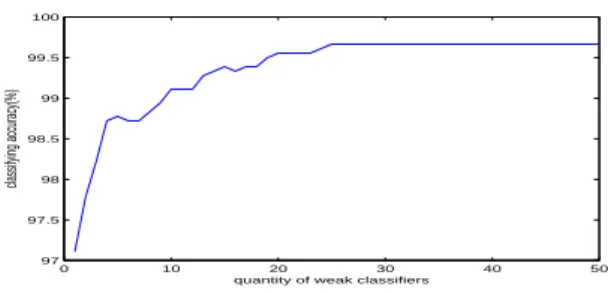
In addition, the stochastic gradient algorithm to enhance the performance bottleneck lies in the number of basic clas-sifiers. We tested the relationship between the number of classifiers and accuracy on the Optdigits data sets (see Fig-ure 1). Classification accuracy was found to significantly increase with the increasement of the number of iteration process. The accuracy rate increase is not very obvious, even stagnation when iterations is up to 25. So, it is nec-essary to control the total number of iterations through the detection accuracy of the test sample in the training phase. To this end we introduce random sampling in order to op-timize the training error detection methods to improve the stochastic gradient iterations through the step 11 to 16 (see Algorithm 1).

0 10 20 30 40 50

97

quantity of weak classifiers

Figure 1: The relationship between classifying accuracy and quantity of weak classifiers on Optdigits data set.

3 Enhance image classification

based on fast stochastic gradient

boosting

This article discusses the general image classification methods and processes, we propose a fast stochastic gra-dient boosting to enhance image classification based the framework in Figure 2. First, we the extract image

fea-start

Image sets

1: Extracting image PHOW feature

PHOW feature sets

2: Additive kernel transformation

Image descriptor sets

4: Model training based on Fast Stochastic Gradient Boosting with training sets

Trained models

Model Framework

Using models 5: Model classification

Classifying results

end

Figure 2: The framework of image classification.

(5)

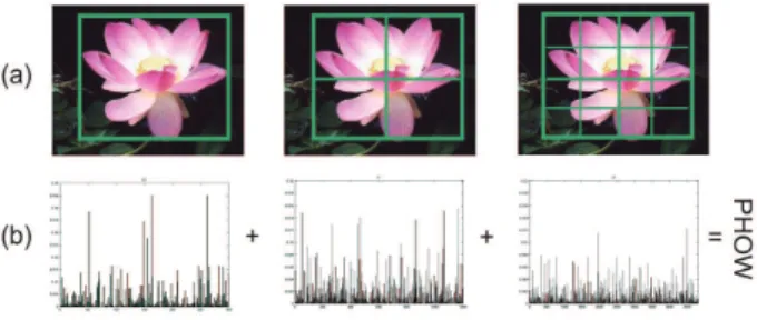
Figure 3: Image appearance representation based on PHOW.

x, y, Additive kernel is defined as :

K(x, y) = B

X

b=1

k(xb, yb) (1)

Here,bis a histogram of the number of each sub-grid,Bis the total number of sub-grid,xb,ybis the distribution of

ev-ery little grid,k:R+ 0×R

+ 0 −→R

+

0 in the non-negative real number is a positive definite kernel. We proposed Vedaldi’s

χ2_{kernel transform for feature transformation.}

Finally, We use the feature descriptors for fast stochastic gradient boosting algorithm to enhance the performance of classification model. At testing stage, we also need to ex-tract features, then do kernel transformation of PHOW to form feature descriptor, again use a classification model to prediction. Our biggest advantage is that the entire frame-work is simple, good computing performance, and suitable for multi-category classification of natural images.

3.1 Experimental data sets

Optdigits data set[27] is a collection of data set standard-ized extracting of bit image by the U.S. National Institute of Standards and Technology handwritten Optical Charac-ter Recognition. It has 64 positive integers of feature infor-mation, the range is from 0 to 16. This data set consists of 5620 instances, belonging to 10 categories. we randomly selected 10%, 20% and 30%, 40% and 50% of total sample as the training sample, and the rest for test samples.

15-Scenes data set[28] is processed in accordance with the flow chart of our proposed framework (see Figure 2). The original 15-Scenes data set consists of 15 data cate-gories, a total of 4485 images. We randomly select 10% and 20%, 30% and 40% and 50% of each class sample for the training sample, and the rest used to do the test samples. We use the PHOW descriptor for image features to describe each image. After kernel transformation with additive eventually, we get 36,000 dimensional feature de-scriptors for a single image.

3.2 Parameters

1) Maximum decision tree depth: The default value was set to 1. With the value increase, classification accuracy

and running time will increase. We set maximum depth to 2, 4, 6, 8, 10, 12, 14, 16, 18 and 20 respectively. We found the highest accuracy rate when the maximum depth is 10. With similar way, we found that entropy rules of split consideration criterion get better performance.

2) The maximum depth of random random forest was similar with decision tree. The number of decision trees: we tested the value of 20, 40, 60, 80, 100, 120, 140, 160, 180 and 200 respectively. We found that the number in-creases, the execution time also inin-creases, and after over the value of 100, the improvement of the accuracy rate was not obvious. So we set it to 100. The accuracy of the ran-dom forest was used to control the iteration. We tested the value of 0.0001, 0.001, 0.01 and 0.1 respectively. We found that the smaller the value was, the longer the execution time was, and after over the value of 0.001, the accuracy had no substantially change. We set it to 0.001.

3) The extreme random tree’s settings was similar with random forests for consistent comparing standard.

4) With similar ways, we found that we get better perfor-mance (good balance in accuracy and running time) when the stochastic gradient enhance maximum tree depth is set to 10, cross entropy loss chosen for loss function type , 0.1 set to shrinkage factor, 0.8 set to proportional sampling un-der, and 100 chosen for maximum lift.

5) Similarly, in order to enhance the fast stochastic gra-dient boosting based on the stochastic gragra-dient boosting, the control error was set to: 0.0001, random verification sampling ratio was set as follows: 50%.

3.3 Experimental setup

We used C++ of Microsoft visual studio 2012 to pro-gram with opencv2.4.3[24], Intel TBB[25]and darwin 1.6 platform[26]. We tested results in win7 (64) platform with hardware of Intel P6100 dual-core CPU and 6GB memory. We converted the data set to comma delimitedM×Nin the form of a text file,Mrepresented the number of (ie, the number of records) data rows,N was the number of each data attribute values. The final column was class marker.

We used TBB parallel libary for parallel processing. In Algorithm 1: At steps of 2,5,7,13, We used TBB withtbb::

parallel_f or. At step 6 involving recursive tree, we used TBB withtbb::task_listto achieve parallelism.

In order to better reflect the effectiveness of the pro-posed framework, we have two types of data sets in the test, Optdigits for low-dimensional data, 15-Scenes for high-dimensional data, and extract the sample test to verify the practicality for different circumstance.

(6)

10 15 20 25 30 35 40 45 50 97

percentage of training sample(%)

(a) Total accuracy

10 15 20 25 30 35 40 45 50

0 5 10 15 20 25 30 35

training time(s)

dt rf et gbt pgbt pcgbt

(b) Training time

Figure 4: The performances of six algorithms on Optdigits.

3.4 Experimental results and analysis

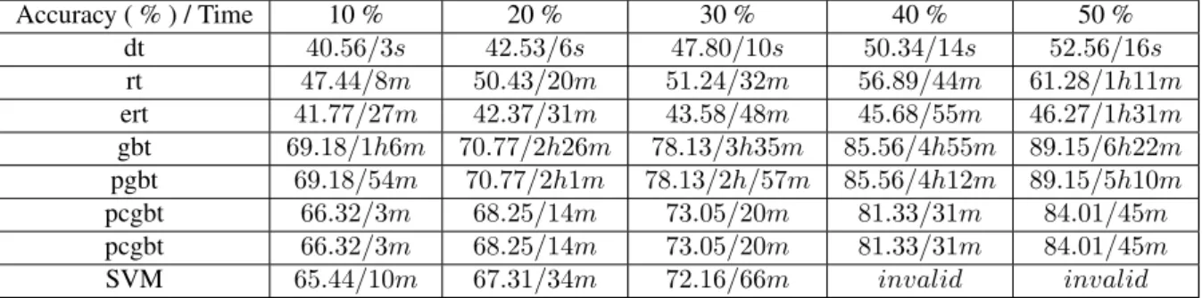
Table 2-3 is a averaged results tested three times under the same conditions. Where h is hours, m represents minutes, s is seconds, ms is milliseconds, such as: 1h2m3s4ms rep-resents 1 hour, 2 minutes, 3 seconds, and 4 milliseconds. dt is a decision tree, rt is random forests, et is extreme ran-dom tree, gbt is stochastic gradient boosting, pgbt is fast stochastic gradient boosting, pcgbt is the fast stochastic gradient boosting with error check, and SVM is support vector machine.

1) With increase of the proportion of each sampling, al-gorithm accuracy rate increases, however the correspond-ing traincorrespond-ing time also increases. This indicates the ade-quacy of the training sample for classification accuracy is critical, but the running performance will be affected in the training. In practical applications, we should consider the two factors, and try to find the best balance between them.

2) Total accuracy comparison: As can be seen from Ta-ble 2-3 and Figure 4-5 (a), stochastic gradient boosting and fast stochastic gradient boosting have same overall accu-racy. Overall accuracy on 15-Scenes data set from high to low is stochastic gradient boosting, stochastic gradient boosting with error detection, random forest, extreme ran-dom tree and decision tree. The main difference on Optdig-its data set lies in that decision tree was significantly better than random forests, furthermore compared with random gradient boosting, the accuracy of our stochastic gradient boosting with error check also has a certain decline of ac-curacy, but is still significantly better than the decision tree and random forest.

3) Running time comparison: From Table 2 to 3 and Fig-ure 4 to 5 (b) shows that the training runtime performance

10 15 20 25 30 35 40 45 50

40

(a) Total accuracy

10 15 20 25 30 35 40 45 50

0 50 100 150 200 250 300 350 400

training time(m)

dt rf et gbt pgbt pcgbt

(b) Training time

Figure 5: The performances of six algorithms on 15-Scenes.

in descending order is decision tree, fast stochastic gradi-ent boosting with error detection, random forests and ran-dom forests extreme, fast stochastic gradient boosting and stochastic gradient boosting. Stochastic gradient boosting with error detection is about 10 times fast than the original stochastic gradient boosting on the data set Optdigits and 8 times on 15-Scenes data set.

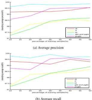
4) Average recall,average precision and total accuracy comparisons: from figure 4 to 7, we can see that the cures have similar curve tendency. This shows that total accuracy basically reflect the performance of classifier on Optdigits and 15-Scenes data set respectively.

5) Comparison with support vector machine: from table 2 and table 3, we can see that the total accuracy of SVM is superior to decision tree, random forest trees and ex-tremely random trees, however inferior to stochastic boost-ing tree based methods. Furthermore, on 15-Scenes data set SVM is failed when the training sampling percentages reach 40% and 50%. On the side of the training time, SVM is slower than decision tree, random forest trees and ex-tremely random trees, but faster the stochastic boosting tree based methods.

4 Conclusions

(7)

algo-10 15 20 25 30 35 40 45 50 97 97.5 98 98.5 99 99.5 100

classifying average precision(%) dt rf et gbt and pgbt pcgbt

(a) Average precision

10 15 20 25 30 35 40 45 50

97 97.5 98 98.5 99 99.5 100

classifying average recall(%) dt rf et gbt and pgbt pcgbt

(b) Average recall

Figure 6: The performances of six algorithms on Optdigits.

rithm. Furthermore, fast stochastic gradient boosting with error detection improves running performance to a new stage, while keeping the overall accuracy comparing to the original stochastic gradient boosting. Experiments testify that our improvement ways are effective and practical.

The main contributions of this paper are :

1) We presents a framework based on PHOW features and fast stochastic gradient boosting for natural image clas-sification. From training sample selection, feature extract-ing, classifier selection to the last performance evaluation, we give a detailed analysis and commentary.

2) We analyze the running performance and bottlenecks of the stochastic gradient boosting. According to the cir-cumstance of bottlenecks and current widely used multi-core computing, we presented modified stochastic gradi-ent boosting to improve the performance of by local paral-lelism.

3) Due to reason of that increasing number of weak clas-sifiers does not always bring better accuracy, and to further reduce the space and time of weak classifier training itera-tions, we introduce an error control mechanism in training phase to reduce the number of iterations of the method at the expense of a certain degree of accuracy degeneration. However, by this way we get further improvement of the running performance.

4) In this paper, a parallel realization of serial algorithm are thoroughly discussed. Taking stochastic gradient boost-ing as example, we proposed a well-established ideas and methods of these kind of problems, namely: 1) to detect bottlenecks, determining the optimization core; 2) the task segmentation, transforming a serial program by paralleliza-tion ideas; 3) implementaparalleliza-tion based on TBB parallel archi-tecture.

10 15 20 25 30 35 40 45 50

40 45 50 55 60 65 70 75 80 85 90

classifying average precision(%)

dt rf et gbt and pgbt pcgbt

(a) Average precision

10 15 20 25 30 35 40 45 50

40 45 50 55 60 65 70 75 80 85 90

classifying average recall(%)

dt rf et gbt and pgbt pcgbt

(b) Average recall

Figure 7: The performances of six algorithms on 15-Scenes.

References

[1] R. M. Haralick, K. Shanmugam, I. Dinstein. Tex-tural features for image classification.IEEE Trans-actions on Systems, Man and Cybernetics,(1973), SMC-3(6):610−621

[2] T. Ojala, M. Pietikainen, T. Maenpaa. Multiresolution gray-scale and rotation invariant texture classifica-tion with local binary patterns.IEEE Transactions on Pattern Analysis and Machine Intelligence, (2002), 24(7): 971−87

[3] D. G. Lowe. Distinctive image features from scale-invariant keypoints.International journal of computer vision, (2004), 60(2): 91−110

[4] N. DALAL, B. TRIGGS. Histograms of oriented gra-dients for human detection. In: Proceedings of the IEEE Computer Society Conference on Computer Vi-sion and Pattern Recognition, New York, USA: IEEE, (2005). 886−893.

[5] T. Leung, J. Malik. Representing and recogniz-ing the visual appearance of materials usrecogniz-ing three-dimensional textons.International journal of com-puter vision, (2001), 43(1): 29−44.

[6] L. Nanni, A. Lumini. Heterogeneous bag of features for object/scene recognition.Applied Soft Comput-ing, (2013), 13(4): 2171−2178.

(8)

In-[9] A. Vedaldi, A. Zisserman. Efficient additive ker-nels via explicit feature maps.IEEE Transactions on Pattern Analysis and Machine Intelligence, (2012), 34(3): 480−492.

[10] P. Kamavisdar, S. Saluja, S. Agrawal. A Sur-vey on Image Classification Approaches and Tech-niques.In: International Journal of Advanced Re-search in Computer and Communication Engineer-ing, (2012), 2(1):1005−1009.

[11] R. M. Haralick, K. Shanmugam, I. H. Dinstein. Tex-tural features for image classification.IEEE Trans-actions on Systems, Man and Cybernetics, (1973), SMC-3(6): 610−621.

[12] G. Ridgeway. Generalized Boosted Models: A guide to the gbm package [Online], available: https://code.google.com/p/ gradientboostedmodels/.

[13] O. Chapelle, P. Haffner, V. N Vapnik. Support vec-tor machines for histogram-based image classifica-tion.IEEE Transactions on Neural Networks, (1999), 10(5): 1055−1064.

[14] G. M. Foody, A. Mathur. A relative evaluation of multiclass image classification by support vector ma-chines. IEEE Transactions on Geoscience and Re-mote Sensing, (2004), 42(6): 1335−1343.

[15] L. Breiman, J. Friedman, C. J. Stone, et al. Classi-fication and regression trees.New York: Chapman & Hall/CRC, (1984).

[16] R. Lawrence, A. Bunn, S. Powell, et al. Classification of remotely sensed imagery using stochastic gradient boosting as a refinement of classification tree anal-ysis.Remote sensing of environment, (2004), 90(3): 331−336.

[17] L. Breiman. Bagging predictors. Machine learning, (1996), 24(2): 123−40

[18] L. BREIMAN. Random forests. Machine learning, (2001), 45(1): 5−32.

[19] P. GEURTS, D. ERNST, L. WEHENKEL. Extremely randomized trees. Machine learning, (2006), 63(1): 3−42.

[20] E. Bauer, R. Kohavi. An empirical comparison of vot-ing classification algorithms: Baggvot-ing, boostvot-ing, and variants.Machine learning, (1998), 36(1): 105−139.

(2012):553−562

[23] J. H. Friedman. Stochastic gradient boosting. Compu-tational Statistics and Data Analysis, (2002), 38(4): 367−378.

[24] D. Abram, T. Pribanic, H. Dzapo, M. Cifrek. A brief introduction to OpenCV.In: Proceedings of the 35th International Convention, Opatija,(2012). 1725−1730.

[25] J. Reinders.Intel threading building blocks: outfitting C++ for multi-core processor parallelism. Graven-stein: O’Reilly Media, Inc. (2010).

[26] S. Gould. DARWIN: A Framework for Machine Learning and Computer Vision Research and De-velopment.Journal of Machine Learning Research, (2012). 13(12): 3499−3503.

[27] K. Bache, Lichman. UCI machine learning reposi-tory[Online]. http://archive.ics.uci.edu/ml.(2013).

(9)

Modules Sampling calculating the gradient

weak classifier training

computing residuals

Prediction

Running count 100 1000 1000 1000 100

Serial Time 170us 2.2ms 62ms 1.6ms 0.5ms

Parallel Time 150us 1.3ms 50ms 1.2ms 0.4ms

Table 1: Serial and parallel executing time of bottleneck modules on Optdigits data set.

Accuracy ( % ) / Time 10 % 20 % 30 % 40 % 50 %

dt 99.16/6.0ms 99.20/17.0ms 99.24/19.9ms 99.37/25.0ms 99.52/34.0ms

rt 97.37/933ms 98.19/2.0s 98.42/3.1s 98.50/4.3s 98.54/5.5s

ert 97.27/1.4s 97.68/2.8s 98.47/4.2s 98.54/5.8s 98.72/7.2s

gbt 99.60/6.1s 99.84/12.2s 99.85/18.5s 99.82/25.8s 99.85/33.2s

pgbt 99.60/4.5s 99.84/10.2s 99.85/16.5s 99.82/20.4s 99.85/29.3

pcgbt 98.55/206ms 98.88/1.2s 99.42/1.3s 99.50/2.3s 99.50/4.5s

SVM 98.52/406ms 98.60/1.8s 98.62/2.1s 98.73/3.5s 98.80/6.5s

Table 2: The Comparison of accuracy and running time of six algorithms on Optdigits with different sampling.

Accuracy ( % ) / Time 10 % 20 % 30 % 40 % 50 %

dt 40.56/3s 42.53/6s 47.80/10s 50.34/14s 52.56/16s

rt 47.44/8m 50.43/20m 51.24/32m 56.89/44m 61.28/1h11m

ert 41.77/27m 42.37/31m 43.58/48m 45.68/55m 46.27/1h31m

gbt 69.18/1h6m 70.77/2h26m 78.13/3h35m 85.56/4h55m 89.15/6h22m

pgbt 69.18/54m 70.77/2h1m 78.13/2h/57m 85.56/4h12m 89.15/5h10m

pcgbt 66.32/3m 68.25/14m 73.05/20m 81.33/31m 84.01/45m

SVM 65.44/10m 67.31/34m 72.16/66m invalid invalid

(10)