Finite Difference Schemes for the Determination of Thermal Coefficient and Analysis of its Variation with Time

Finite Difference Schemes for the Determination of Thermal

Coefficient and Analysis of its Variation with Time

M.Usman1*, M.O.Ahmed2, M.Rafiq3, Sumera.K2 and Mumtaz.A2

1. Department of Basic Sciences & Humanities, University of Engineering and Technology, Lahore (KSK Campus), Pakistan.

2. Department of Mathematics, University of Engineering and Technology, Lahore, Pakistan. 3. Faculty of Engineering, University of Central Punjab, Lahore, Pakistan.

* Corresponding author: [email protected]

Abstract

In this paper, numerical solution of thermal conduction problem has been analyzed. Three Finite difference schemes have been derived for the determination of thermal coefficient and for temperature distribution at different time levels. Moreover, by using derived schemes a test problem has been solved and computed results have been compared with exact solutions for different time level, it reveals accuracy of these schemes as well as the physical behavior of the test problem. The general pattern which has been observed is that with passage of time temperature distribution increases.

Key Words

: Finite differences, Crank-Nicolson Scheme, Thermal conductivity/diffusivity

1. Introduction

Analysis of the variation of diffusion coefficient with time plays an important role for determining nature of the material; [4, 6, 7] these types of problems are encountered in physical phenomena like heat conduction problems in different materials (conductivity of medium), reaction diffusion equation problem etc., [8]. In this paper a thermal conduction problem is under consideration in which temperature distribution and thermal coefficient are simultaneously measured by finite difference techniques.

Consider the Problem

F T T X

T T

T ∂ < < < < ∂

= ∂ ∂

0 . 1 0 , ) ( ˆ

2 2_ψ α ψ

(1)

with initial condition l X X F

X,0)= ( ),0≤ ≤ (

ψ (2)

with boundary conditions

F T T T G

T)= ( ),0≤ ≤ ,

0

( ₀

ψ (3)

F T T T G T

l, )= ( ),0≤ ≤

( ₁

ψ (4)

where l=length of rod, T_F= final temperature with additional measurement

F T T T M T

X , )= ( ),0≤ ≤ ( *

ψ (5)

Where F,G₀(T), G₁(T) and M(T) are known functions but ψ(X,T) and αˆ(T) are unknown. Here

) ( ˆ T

α is called thermal or diffusion coefficient while

) , (X T

ψ is known as temperature distribution. Cannon [1] converted the problem (1) to (5) to a non-linear integral equation for αˆ(T). Yin and Cannon [2] developed finite element technique for the solution of the problem (1) – (5). Deghan [3] analyzed the problem for particular time level. The problem (1) to (5) can be used for determination of unknown properties such as the coefficient αˆ(T)

which represents some physical quantity like the conductivity or diffusivity of medium. A case when unknown diffusivity depends upon temperature distribution was discussed by Fatuallyev [5]. In this paper a test problem is also solved by derived finite difference schemes for different time levels, solutions are presented in tables which reveal that diffusivity/conductivity varies with time and indirectly with temperature.

2. Derivation of Explicit Finite

Difference Scheme

For the derivation we use following notations

= =

= , ( ) , ( )

) ,

(X_i T_j ψ_j M T_j M j G₀ T_j

ψ

j j i i j j

j _{G T G F X F T} G₀, ₁( )= ₁, ( )= αˆ( )αˆ

, .... , 2 , 1 , 0 m i ih

X_i = =

N j

jk

T_j= , =0,1,2,...

Here is a point that can also be chosen as mesh point, [X]↑#=i_↓#h,where1≤i_↓#≤m−1

Equation (5) can be written as

) ( _j j j

h

io =M =M T ψ

Differentiating above equation w.r.t “T”, we get

) , ( ) , ( )

(Tj T X*Tj T i*hTj

M′ =ψ =ψ (6)

So from equation (1), we have ) , ( ) ( ˆ )

(T T X*T

M′ =α ψ_xx (7)

Let us now assume that 0 ) , (X* T ≠ xx

ψ , hence from equation (7), we obtain F xx T T T X T M

T = ′ 0< < ) , ( ) ( ) ( ˆ * ψ

α (8)

So the inverse problem (1) to (5) is equivalent to the following problem

) , ( ) , ( ) ( ) ,

( _* X T

T X T M T X xx xx T ψ ψ

ψ = ′ (9)

F T T l

X < < <

< , 0

0

with initial and boundary conditions are l

X X F

X,0)= ( ),0≤ ≤ (

ψ (10)

F T T T G

T)= ( ), 0≤ ≤ ,

0

( 0

ψ (11)

F T T T G T

l, )= ( ),0≤ ≤

( ₁

ψ (12)

Step 2.1 Transformation Let ) , ( ) ,

(X T ψxx X T

µ = (13)

) , (X T

ψ and µ(X,T) are continuous in given domain.

( )

T T X X T T ∂ ∂ ∂ ∂ = ⎟ ⎟ ⎠ ⎞ ⎜ ⎜ ⎝ ⎛ ∂ ∂ ∂ ∂ = ∂ ∂

= µ ψ _ψ

µ ) ( ) ( 2 2 2 2

Using eq (9), we get

) )( ( ) , ( ) ( ) , ( ) ( 2 2 * * 2 2 xx xx xx T X T X T M T X T M

X µ ψ

ψ ψ µ ∂ ∂ ′ = ⎟ ⎟ ⎠ ⎞ ⎜ ⎜ ⎝ ⎛ _′ ∂ ∂ = F xx

T X l T T

T X

T

M′ _{≤ ≤ ≤ ≤}

= , 0 , 0

) , ( ) ( * µ µ

µ (14)

Finally our problem becomes

⎪ ⎪ ⎪ ⎪ ⎭ ⎪⎪ ⎪ ⎪ ⎬ ⎫ ≤ ≤ ′′ = ≤ ≤ ′′ = ≤ ≤ ′′ = ≤ ≤ ≤ ≤ = ′ ′′ ′ ′′ ′ F T M T G F T M T G F xx T x T M T T T T X T T T T X T X X F X are conditions boundary and initial with T T X 0 ), , ( ) , 1 ( 0 ), , ( ) , 0 ( 1 0 ), ( ) 0 , ( 0 , 1 0 , ) ( ) ( ) ( ) ( ) , ( ) ( 1 0 µ µ µ µ µ µ µ _µ

)

15

(

Applying forward difference approximation for T

µ and central difference approximation for µ_xx, at time level j respectively. So our problem becomes

[

]

[

j

]

i j i j i j j j i j i k _h Q 1 1 * 2 1 1 ₂ + −

+ _{− = µ − µ +µ}

µ µ

µ (16)

1 0

, 1

1≤i≤m− ≤j≤N− where

) ( _j

j _{M T}

Q = ′ (17)

with initial condition

m i

X

F _i

i0= ′′( ), =0,1,2,...

µ (18)

and with boundary conditions

0 ) ( ) ( 0 0 _≥ ′ ′ = j T H T G j j i

µ (19)

0 ) ( ) ( 1 _≥ ′ ′ = = j T H T G j j j m j i µ

µ (20)

where j j j j j T M Q T H * * ) ( ) ( µ µ ′ = =

′ (21)

j i i j i i j i h X X h X X h 1 0 0 0

0) ( )

( # * * + − + − −

= µ µ

µ (22)

where ] , [ ₁ # 0 0 i +

i X

X E X

Step 2.2

Equation (16) takes the form j i j i j i j

i v 1 v v 1

1 ) 2 1 ( ₊ −

+ _{= µ + − µ + µ}

µ (23)

where 1≤i≤m−1,0 ≤j≤N−1 and

j j h k Q v * 2_µ

= (24)

Step 2.3

In order to find ψ from µ, we have to solve following B.V.P 0 , 0 ), , ( ) ,

(X T = X T <X<l T>

xx µ

ψ (25)

F T T T

G

T)= ( ), 0≤ ≤ ,

0

( ₀

ψ (26)

F T T T

G

T)= ( ), 0≤ ≤ ,

1

( ₁

ψ (27)

So by using finite differences, equation (25) becomes 1 , 1 1 , 2 2 1

1− + + _{= ≤ ≤ − ≥}

− _{i m j}

h j i j i j i j

i ψ ψ _µ

ψ

(28)

with boundary conditions

0 ,

0 0=G j≥

j j

ψ (29)

0 ,

1 ≥

=Gj j j

m

ψ (30)

where µ_ij, is the solution of equation (23).

Step 2.4

Next we find αˆ(T) or αˆ

( )

(T)_j by using equation (8) i.e.

1 , ) , ( ) ( ) , ( ) ( ) ( ˆ * * ≥ ′ = ′ = j T X T M T X T M T j j j xx j j µ ψ

α (31)

3. Derivation of Backward Implicit

Finite Difference Scheme

Procedure of this scheme up to equation (15) is same as of pervious scheme. Now applying backward difference approximation for µ_T at time level j+1 and central difference approximation for µ_xx at time level j+1, therefore

1 1 1 1

1 (1 2 )

+ + + + − + + − − = j i j i j i j

i vµ vµ vµ

µ (32)

for 1≤i≤m−1, j=0,1,2,...,N−1,

where _j

j h k Q v * 2_µ

= with initial and boundary conditions given in equations (18), (19), (20). Remaining steps are same as we did in explicit finite difference scheme.

4. Derivation of another (Crank

Nicolson) Implicit Finite Difference

Scheme

Procedure of this scheme up to equation (15) is same as of explicit scheme. This scheme is derived by averaging forward difference scheme at time level ‘j’ and backward implicit scheme at time level ‘j+1’. So finally we get

= −

+ +

− ₋+ + ₊+1

1 1 1

1 2(1 )

j i j i j

i v v

vµ µ µ

j i j i j

i v v

vµ₋₁+2(1+ )µ + µ₊₁ (33) 0

1 , 1

1≤i≤m− N− ≥j≥

where _j

j h k Q v * 2_µ =

with initial and boundary conditions as given in equations (18), (19), (20). Remaining steps are same as we did in explicit finite difference scheme.

5. Test

Problem

Consider the given partial differential equation

T X

T T

T ∂ < < <

∂ = ∂ ∂ 0 , 1 0 , ) ( ˆ 2 2_ψ α ψ

with I.C as ψ(X,0)=F(X)=ex, 0≤ X ≤1 with B.Cs as

. 0 , 1 ) ( ) , 0

( T =G₀ T = +T T≥

ψ 0 , ) 1 ( ) ( ) , 1

( T =G₁T = +T e1 T ≥

ψ

with additional measurement as Let us Find αˆ(T)

And ψ(X,T).

Exact solution: ) 1 ( ) ,

(X T =ex +T

ψ and

t T + = 1 1 ) ( ˆ α

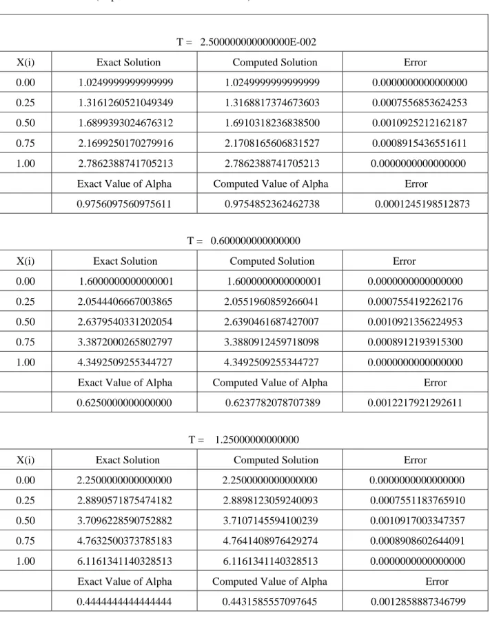
Table 1 Test Problem (Explicit Finite Difference Scheme)

T = 2.500000000000000E-002

X(i) Exact Solution Computed Solution Error

0.00 1.0249999999999999 1.0249999999999999 0.0000000000000000 0.25 1.3161260521049349 1.3168817374673603 0.0007556853624253 0.50 1.6899393024676312 1.6910318236838500 0.0010925212162187 0.75 2.1699250170279916 2.1708165606831527 0.0008915436551611 1.00 2.7862388741705213 2.7862388741705213 0.0000000000000000

Exact Value of Alpha Computed Value of Alpha Error

0.9756097560975611 0.9754852362462738 0.0001245198512873

T = 0.600000000000000

X(i) Exact Solution Computed Solution Error

0.00 1.6000000000000001 1.6000000000000001 0.0000000000000000 0.25 2.0544406667003865 2.0551960859266041 0.0007554192262176 0.50 2.6379540331202054 2.6390461687427007 0.0010921356224953 0.75 3.3872000265802797 3.3880912459718098 0.0008912193915300 1.00 4.3492509255344727 4.3492509255344727 0.0000000000000000

Exact Value of Alpha Computed Value of Alpha Error

0.6250000000000000 0.6237782078707389 0.0012217921292611

T = 1.25000000000000

X(i) Exact Solution Computed Solution Error

0.00 2.2500000000000000 2.2500000000000000 0.0000000000000000

0.25 2.8890571875474182 2.8898123059240093 0.0007551183765910

0.50 3.7096228590752882 3.7107145594100239 0.0010917003347357

0.75 4.7632500373785183 4.7641408976429274 0.0008908602644091

1.00 6.1161341140328513 6.1161341140328513 0.0000000000000000

Exact Value of Alpha Computed Value of Alpha Error

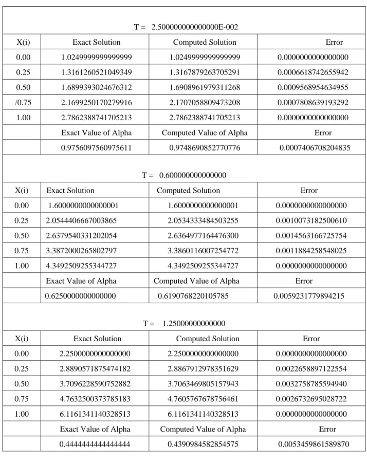
Table 2 Test Problem (Implicit Finite Difference Scheme)

T = 2.500000000000000E-002

X(i) Exact Solution Computed Solution Error

0.00 1.0249999999999999 1.0249999999999999 0.0000000000000000

0.25 1.3161260521049349 1.3167879263705291 0.0006618742655942

0.50 1.6899393024676312 1.6908961979311268 0.0009568954634955

/0.75 2.1699250170279916 2.1707058809473208 0.0007808639193292

1.00 2.7862388741705213 2.7862388741705213 0.0000000000000000

Exact Value of Alpha Computed Value of Alpha Error 0.9756097560975611 0.9748690852770776 0.0007406708204835

T = 0.600000000000000

X(i) Exact Solution Computed Solution Error

0.00 1.6000000000000001 1.6000000000000001 0.0000000000000000

0.25 2.0544406667003865 2.0534333484503255 0.0010073182500610

0.50 2.6379540331202054 2.6364977164476300 0.0014563166725754

0.75 3.3872000265802797 3.3860116007254772 0.0011884258548025

1.00 4.3492509255344727 4.3492509255344727 0.0000000000000000

Exact Value of Alpha Computed Value of Alpha Error

0.6250000000000000 0.6190768220105785 0.0059231779894215

T = 1.25000000000000

X(i) Exact Solution Computed Solution Error

0.00 2.2500000000000000 2.2500000000000000 0.0000000000000000 0.25 2.8890571875474182 2.8867912978351629 0.0022658897122554 0.50 3.7096228590752882 3.7063469805157943 0.0032758785594940 0.75 4.7632500373785183 4.7605767678756461 0.0026732695028722 1.00 6.1161341140328513 6.1161341140328513 0.0000000000000000

Exact Value of Alpha Computed Value of Alpha Error

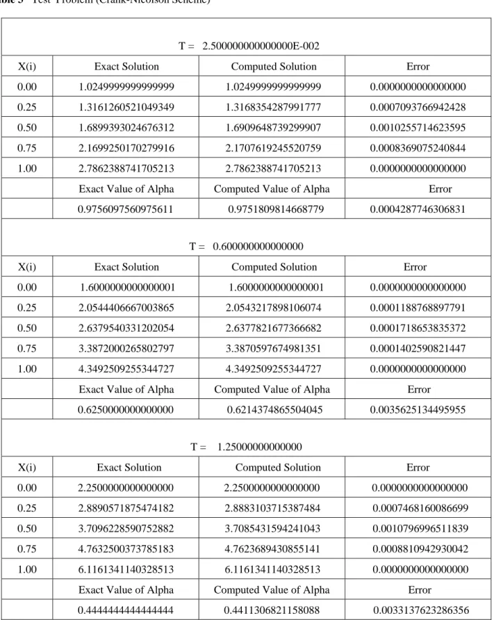
Table 3 Test Problem (Crank-Nicolson Scheme)

T = 2.500000000000000E-002

X(i) Exact Solution Computed Solution Error

0.00 1.0249999999999999 1.0249999999999999 0.0000000000000000 0.25 1.3161260521049349 1.3168354287991777 0.0007093766942428 0.50 1.6899393024676312 1.6909648739299907 0.0010255714623595 0.75 2.1699250170279916 2.1707619245520759 0.0008369075240844 1.00 2.7862388741705213 2.7862388741705213 0.0000000000000000

Exact Value of Alpha Computed Value of Alpha Error

0.9756097560975611 0.9751809814668779 0.0004287746306831

T = 0.600000000000000

X(i) Exact Solution Computed Solution Error

0.00 1.6000000000000001 1.6000000000000001 0.0000000000000000 0.25 2.0544406667003865 2.0543217898106074 0.0001188768897791 0.50 2.6379540331202054 2.6377821677366682 0.0001718653835372 0.75 3.3872000265802797 3.3870597674981351 0.0001402590821447 1.00 4.3492509255344727 4.3492509255344727 0.0000000000000000

Exact Value of Alpha Computed Value of Alpha Error

0.6250000000000000 0.6214374865504045 0.0035625134495955

T = 1.25000000000000

X(i) Exact Solution Computed Solution Error

0.00 2.2500000000000000 2.2500000000000000 0.0000000000000000

0.25 2.8890571875474182 2.8883103715387484 0.0007468160086699

0.50 3.7096228590752882 3.7085431594241043 0.0010796996511839

0.75 4.7632500373785183 4.7623689430855141 0.0008810942930042

1.00 6.1161341140328513 6.1161341140328513 0.0000000000000000

Exact Value of Alpha Computed Value of Alpha Error

6. Results and Discussion

Computed results of the problem obtained by using derived Finite Difference Schemes and their comparison with exact solutions for different time level are presented in Tables 1-3. It is clear from the tables that approximate results obtained by three derived Finite difference schemes are very close to exact results which show the accuracy and applicability of the schemes. In Graphs 1 to 3, points indicate the numerical values of thermal coefficient

α

ˆ

(T) while lines indicate its exact values. It is clear from all three plots that numerical values of

α

ˆ

(T) obtained by three FDMs are very close to exact values for small time step that reveals high accuracy of these schemes for test problem. Graphs also demonstrate that value of thermal coefficient decreases with the passage of time.

7. Conclusion

Numerical solutions of thermal conduction problem are presented in Tables 1-3, from tables it revealed that:

• With the passage of time temperature increases and thermal coefficient decreases so the material in this heat conduction problem resemble with conductor.

• For T=0.025, Backward difference implicit scheme gives better approximation for Ψ(X, T), while for T=0.6 & 1.25, Crank-Nicolson implicit scheme gives better approximation for

Ψ(X, T).

• For T=0.025, 0.6 & 1.25 better approximation for αˆ(T) are given in descending order by Explicit Finite Difference Scheme, Crank- Nicolson scheme and finally by Backward Difference Implicit Scheme.

References

[1] J.R.Cannon, 1963. Determination of an unknown coefficient in parabolic differential equation, Duke Math J 30, 313-323.

[2] J.R.Cannon and H.M.Yin, 1990. Numerial solution of some parabolic inverse problems, Numer Methods of Partial Differential equation 2,177-191.

[3] Mehdi Deghan, 2005. Identification of a Time –dependent Coefficient in a partial differential equation subject to an Extra Measurment, Numer Methods Partial Differential Eq 21, 611-622.

[4] M.A.Rana, Rashid Qamar, A.A. Farooq, A.M. Siddiqui. 2011. Finite-difference analysis of natural convection flow of viscous fluid in a porous channel with constant heat source, Applied Mathematics Letters 24, 2087-2092.

[5] A.G. Fatuallyev, 2002. Numerical procedure for the determination of an unknown coefficient in Parabolic equation, Comput Phys Commum 144(1),29-33.

[6] P.B.Patial and U.P.Verma. 2009. “Numerical Computational Method” Revised Edition, Narsoa.

[7] R. L. Burden and J. D. Faires, 2011. “Numerical Analysis” 8th edition, PWS, Publishing company , Bostan.

[8] M.K.Jain, 1991. “Numerical Solution of Differential Equations” 2nd edition, Willy Estern Limited.