Sharif University of Technology
Scientia IranicaTransactions A: Civil Engineering www.scientiairanica.com
Development of nonlinear transfer matrix method for
inelastic analyses of beams
M. Kwon
a, J. Kim
a;, H. Seo
aand S. Limkatanyu
ba. Department of Civil Engineering, ERI, Gyeongsang National University, South Korea.
b. Department of Civil Engineering, Faculty of Engineering, Prince of Songkla University, Thailand. Received 6 August 2013; received in revised form 10 June 2014; accepted 20 October 2014
KEYWORDS Material nonlinear; Stiness matrix; TMM (Transfer Matrix Method); Nonlinear analysis; Beam model.
Abstract. The objective of this study is to develop a material-nonlinear-analysis algorithm based on the Transfer Matrix Method (TMM). This newly developed algorithm can be used to perform nonlinear analyses of continuous beam systems. The nonlinear transfer matrix is derived from the general frame stiness matrix, and the Gauss-Lobatto integration scheme is employed for numerical integration. In the TMM, the system equation has a constant number of system unknowns, regardless of the total degree-of-freedom number in the structure and the system response (either linear or nonlinear). As a result, TMM can be used eciently, both for linear and nonlinear structural analyses. In this study, a secant nonlinear algorithm, required in nonlinear TMM, is employed, due to its good compromise between the convergence rate and numerical stability. To verify the accuracy and eciency of the developed TMM, four numerical examples are selected and analyzed. The analysis results are compared with those obtained by the highly accurate exibility-based frame model, in terms of global and local responses.
c
2015 Sharif University of Technology. All rights reserved.
1. Introduction
Regarded as the most powerful numerical tool, the nite element method has been widely used by re-searchers to analyze complex structural systems. How-ever, its use by practicing engineers is still limited, due to the considerable experience required by users to construct a suitable nite element mesh, interpret analysis results, and implement a numerical model. Furthermore, computational costs required in analyz-ing complex structural systems are usually high, even with recent drastic advances in computer technology. This lies in the fact that numerous Degrees Of Free-dom (DOFs) are required to discretize a complex
*. Corresponding author. Tel.: +82 55 7590538; Fax: +82 55 7721799
E-mail address: [email protected] (J. Kim)
structural system, thus, resulting in a large stiness matrix.
In order to remedy this problem, several tech-niques have been developed to reduce the size of the associated stiness matrix in the standard nite element method. These include, for example: the static condensation technique [1], the sub-structuring technique [2], etc. Alternatively, Cheung [3] proposed the so-called \Finite Strip Method (FSM)" as a variant of the standard nite element method to analyze a structure with lesser system unknowns. Another structural-analysis method requiring a smaller system matrix was systematized by Pestel and Leckie [4], which is known as the Transfer Matrix Method (TMM). TMM is of particular interest in this study since the size of the transfer matrix is usually much smaller than that of a structural stiness matrix and is constant, regardless of the total degree-of-freedom number in
the structure and the system response (either linear or nonlinear). This feature is desirable, especially in the framework of nonlinear structural analysis in which high computational cost could become an issue. The transfer matrix is derived based on the general solution of the governing dierential equation [5]. For each element, there are two steps needed to be performed. First, the right-end variables are related to the left-end variables through the transfer matrix. Then, the right-end variables of the current element are used as the boundary conditions for the left-end variables of the next element. These two steps are performed in a successive manner until all system unknowns are computed [6,7]. Since unknown variables at each nodal point can simply be determined using the transfer matrix, the analysis process required in the TMM has to deal only with the transfer matrix of a constant size, regardless of the element number used to discretize the system. This feature renders TMM attractive compared to the standard nite element method. One of the earliest applications of TMM in structural analysis was conducted by Holzer [8] to investigate the torsional vibration problem of crankshafts. Hetenyi [9] also used TMM to study the problem of beams on elastic foundations. During the seventies and eighties, the TMM was successfully applied to the vibration problems of plates by several researchers, but was limited to only linear elastic systems [10-12]. An early extension of TMM to nonlinear structural analysis was the large deection analysis of plates [13-15]. To the authors' knowledge, few researchers have employed TMM to perform inelastic structural analyses. Akintilo and Syngellakis [16] performed inelastic analyses of reinforced concrete coupled shear walls using TMM. Rosignoli [17] employed TMM to analyze launched bridges. Pfeier [18] applied TMM to nonlinear analyses of planar reinforced and prestressed concrete frames, including axial elongation eects. Starossek et al. [19] combined TMM with the displacement method to perform material and geometrical nonlinear analyses of planar reinforced concrete frames.
In this study, an ecient numerical algorithm is developed, with TMM incorporated, for material nonlinear analyses of frame structures. The transfer matrix is derived from the displacement-based element stiness matrix. The nonlinear algorithm implemented is based on the secant iterative scheme, which is more stable than the widely used Newton-Raphson iterative scheme. This is especially true when the material is subjected to yielding and then softening states or behaves elastic perfectly plastic. To verify the accuracy and eciency of the developed TMM model, four numerical examples are investigated. Analysis results obtained using the TMM are compared with those obtained using the exibility-based bre frame model [20] in terms of global and local responses.
Figure 1. Transfer matrix method diagram [21].
2. Derivation of transfer matrix
2.1. General frame element stiness equation Three sets of governing equations used to construct the frame element stiness equation are compatibility, section constitutive, and equilibrium relations. The so-called \Tonti's diagram" of Figure 1 is used to conve-niently represent these governing equations [21]. The virtual displacement principle is employed to represent the integral statement of the element equilibrium, thus, resulting in the element stiness equation. In the element stiness equation, the element stiness matrix serves as the mapping operator between the element nodal displacements and element nodal forces. Details of the derivation of the frame element stiness equation can be found in any nite element textbook [22].
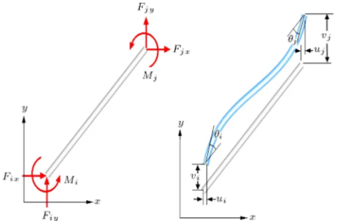
Figure 2 shows a 2-node planar frame element conguration. For each node, there are three dis-placement DOFs and their work-conjugate forces. The
frame element stiness equation is written as:
P = KU: (1)
Following the notation of Figure 2, the element nodal displacements are:
U =UijUj T; (2)
where Ui = fui vi igT and Uj = fuj vj jgT are
arrays containing the displacements at nodes i and j, respectively. Their work-conjugate nodal forces are grouped in the element force vector, P = fPijPjgT.
The element stiness matrix can be expressed as: K =
Z
LB
T(x)k(x)B(x)dx; (3)
where B(x) is the strain-displacement matrix and k(x) is the frame sectional stiness matrix which collects the axial rigidity, EA(x), and exural rigidity, IE(x). 2.2. Partitioned form of the element stiness
matrix
In the TMM, the element stiness equation is modied, such that nodal forces and displacement quantities at each node are grouped in the same vector and are related together through the transfer matrix [23]. This could be accomplished by partitioning the strain-displacement matrix, B(x), as:
B(x) =
Bii(x) Bij(x)
Bji(x) Bjj(x)
; (4)
where: Bii(x) =
dNui(x)
dx 0 0
;
Bij(x) =
dNuj(x)
dx 0 0
;
Bji(x) =
0 d2Ndxvi2(x) d2Ndxi2(x)
;
Bjj(x) =
0 d2Ndxvj2(x) d2Ndxj2(x)
; (5)
in which Nui(x), Nuj(x), Nvi(x), Nvj(x), Ni(x) and
Nj(x) are polynomial interpolation functions for a
2-node planar frame element and are given in any nite element textbook [22].
In accordance with Eq. (4), the element stiness matrix of Eq. (3) can be partitioned as:
K =
Kii Kij
Kji Kjj
; (6)
where each sub-matrix can be expressed as:
Kii =
Z
LBii(x)
TEA(x)B ii(x)dx
+ Z
LBji(x)
TEI(x)B
ji(x)dx;
Kij =
Z
LBii(x)
TEA(x)B ij(x)dx
+ Z
LBji(x)
TEI(x)B
jj(x)dx:
Kji= KTij;
Kjj =
Z
LBij(x)
TEA(x)B ij(x)dx
+ Z
LBjj(x)
TEI(x)B
jj(x)dx: (7)
2.3. Derivation of transfer matrix
Based on the partitioned form of the element stiness matrix of Eq. (6), the element stiness equation of Eq. (1) can be partitioned as:
Pi Pj =
Kii Kij
Kji Kjj
Ui
Uj
; (8)
where Pi = fFix Fiy MigT and Pj = fFjx Fjy MjgT
are arrays containing the forces at nodes i and j, respectively.
The core idea of the TMM is to modify the stiness equation of Eq. (8), such that the forces and displacements at node j are expressed in terms of forces and displacements at node i through the transfer matrix. Therefore, the transfer matrix equation can be expressed in the following form:
Vj= TMVi; (9)
where Vi = fui vi i Fix Fiy MigT and Vj =
fuj vj j Fjx Fjy MjgT are arrays containing the
displacements and forces at nodes i and j, respectively, and TM is the transfer matrix, dened as:
TM =
K 1
ij Kii Kij1
Kji KjjKij1Kii KjjKij1
: (10)
2.4. Numerical integration scheme
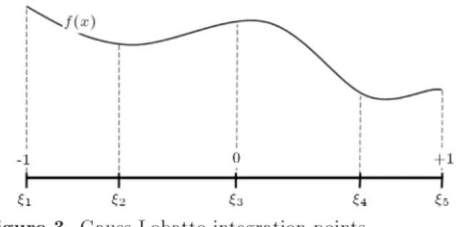
In this study, the numerical integration required in the TMM relies on the Gauss-Lobatto integration scheme, which includes extreme integration points at the element ends, as shown in Figure 3. This numerical integration scheme is preferable to the conventional Gauss integration scheme, since it allows sampling of the element-end response, which, most likely, becomes inelastic [20]. Thus, each sub-matrix of the element
Figure 3. Gauss-Lobatto integration points.
stiness can be written in the Gauss-Lobatto numerical integration form as:
Kii= nIP
X
n=1
Bii(n)TEA(n)Bii(n):J:wn
+
nIP
X
n=1
Bji(n)TEI(n)Bji(n):J:wn;
Kij = nIP
X
n=1
Bii(n)TEA(n)Bij(n):J:wn
+XnIP
n=1
Bji(n)TEI(n)Bjj(n):J:wn;
Kji= KTij;
Kjj = nIP
X
n=1
Bij(n)TEA(n)Bij(n):J:wn
+
nIP
X
n=1
Bjj(n)TEI(n)Bjj(n):J:wn; (11)
where J is the element Jacobian; nIP is the integration point number; n is the integration-point position in
the natural coordinate; and wnis the integration-point
weight.
3. TMM (Transfer Matrix Method)
In TMM, displacement and force quantities at each node are computed by successively multiplying the transfer matrix of each element, enforcing the nodal compatibility with imposed boundary conditions, and satisfying the nodal equilibrium with external loads. 3.1. Boundary condition
The boundary conditions commonly imposed on a beam system can be classied as xed, hinged, roller and free conditions. The boundary condition matrix, An, reaction-force vector, BCn, and prescribed
dis-placement vector, Rn, associated with the boundary
condition at node n are given as [24]:
Fixed:
An=
2
41 0 0 0 0 00 1 0 0 0 0 0 0 1 0 0 0 3 5 ; BCn =0 0 0 bHn bPn bMn T;
Rn=rnu rvn rn T: (12)
Hinged:
An=
1 0 0 0 0 0 0 1 0 0 0 0
;
BCn =0 0 0 bHn bPn 0 T;
Rn=rnu rvn T: (13)
Roller:
An=0 1 0 0 0 0;
BCn =0 0 0 0 bPn 0 T;
Rn= frvngT: (14)
Free:
An=0 0 0 0 0 0;
BCn =0 0 0 0 0 0 T;
Rn= f0gT; (15)
where variables b and r represent the unknown reaction force and the prescribed displacement, respectively. 3.2. Transfer matrix
The schematic notion of the transfer matrix method at each loading stage is conveyed in Figure 4. At a generic node, n, the right nodal variable vector, VR
n,
is computed as the summation of the load vector, Ln,
and boundary condition matrix, BCn.
VR
n = Ln+ BCn; (16)
where the load vector, Ln = f0 0 0 LHn LPn LMn gT,
collects the horizontal force, LH
n, vertical force, LPn,
and moment, LM
n , acting at the node. The left nodal
variable vector, VL
n+1, of node n + 1 is then computed
from the right nodal variable vector, VR
n, of node n
through the following transfer matrix relation: VL
n+1= TMnVnR: (17)
dis-Figure 4. Nodal and element vectors.
placements is satised through the following matrix relation:
An+1VLn+1= Rn+1: (18)
At the end node, the following relation is used to satisfy the equilibrium condition:
AendVRn = Rend; (19)
where:
Aend=
2
40 0 0 1 0 00 0 0 0 1 0 0 0 0 0 0 1 3 5 ;
Rend= f0 0 0gT: (20)
4. Material nonlinearity
In nonlinear structural analysis, the Newton-Raphson iteration method has been widely used since it yields a quadratic convergence characteristic. However, it could become numerically unstable when the tangential stiness of a structure approaches or equals zero. This is in the case when the post-yielding stiness of the force-deformation relation approaches or equals zero. Several researchers have employed dierent approaches to avoid this problem. For example, Manoharan and Dasgupta [25] employed the modied Newton-Raphson iteration method to perform nonlinear consolidation analysis of elastic-perfectly plastic soil. Vecchio [26] used the secant-stiness iteration method to perform inelastic analysis of RC membrane structures. The pros and cons of various iteration methods are thoroughly discussed in Yang and Kou [27].
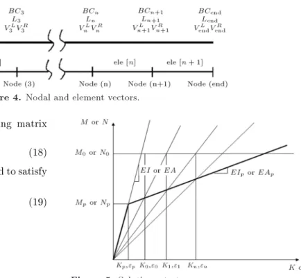
In this study, the secant-stiness iteration method is adopted to solve the nonlinear responses of a beam system, due to its good compromise between conver-gence rate and numerical stability. The schematic representation of the secant-stiness iteration method is shown in Figure 5. Sectional responses (axial and exure) are assumed to be bilinear, as shown in Figure 5. For each section at an integration point, the secant axial stiness and the exural stiness (EAsecant
and EIsecant) are determined. The partitioned element
stiness matrix of Eq. (6) and element transfer matrix of Eq. (10) are computed based on these sectional se-cant properties. The residual work concept is employed as a convergence criterion [27].
Figure 5. Solutions strategy.
5. Numerical examples
Four numerical examples are used to verify the accu-racy and demonstrate the eciency of the proposed material nonlinear transfer matrix method. Corre-lation studies are performed by comparing the ob-tained numerical results with those obob-tained with the exibility-based bre frame element [20]. This exibility-based bre frame element has been widely used in the research community and was implemented into the Open System for Earthquake Engineering Simulation Platform [28]. In all examples, the load-control marching scheme is used for solution procedure, and ve Gauss-Lobatto integration points are employed to perform the required numerical integration.
5.1. Cantilever beam
A cantilever beam of length L = 2 m is subjected to an applied load, P , at its free end, as shown in Figure 6. The beam has a square cross section with dimension of b = h = 50 mm. For the mechanical and strength properties of the beam, an initial elastic modulus of 200 GPa, a yield strength
of 400 MPa, and a strain-hardening ratio of 0.01 are assumed. Four proposed TMM elements are used to represent the cantilever beam, as shown in Figure 6. To ease the global and local response comparisons, four exibility-based frame elements are employed to discretize this cantilever beam, even though one exibility-based element would be sucient to yield accurate results. For the exibility-based model, 15 bers are used to discretize the beam section, while, for the proposed TMM model, exact integration is employed to derive the beam sectional response.
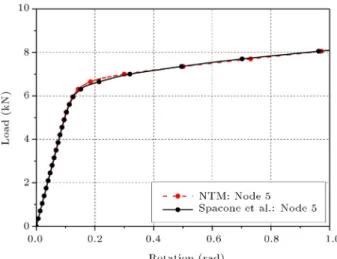
Figures 7 and 8 compare the tip load-displacement and load-rotation curves obtained with the two models. Clearly, global responses obtained with the two models are in good agreement, thus, conrming the accuracy of the proposed TMM model. To investigate local responses of both models, sectional moment-curvature responses, sampled at the rst integration point of each element, are compared in Figure 9. The result clearly
Figure 7. Load vs. displacement for node 5 in the cantilever system in Figure 6.
Figure 8. Load vs. rotation for node 5 in the cantilever system in Figure 6.
shows that the proposed TMM model is capable of well representing local responses.
5.2. Simply supported beam
A simply supported beam of length L = 3 m is subjected to a four-point bending loading, as shown in Figure 10. The beam has a rectangular cross section and is 40 mm wide and 100 mm thick. For the mechanical and strength properties of the beam, an initial elastic modulus of 210 GPa, a yield strength of 420 MPa, and a strain-hardening ratio of 0.002 are assumed. Six proposed TMM elements are used to represent the beam, as shown in Figure 10. To expedite the global and local response comparisons, six exibility-based frame elements are employed to discretize this beam, even though a mesh with fewer el-ements would be sucient to produce accurate results. Two concentrated forces are applied at nodes 3 and 5. For the exibility-based model, 15 bers are used to discretize the beam section, while, for the proposed TMM model, exact integration is employed to derive the beam sectional response.
The load-displacement response at node 3 and load-rotation response at node 5 obtained with the two models are shown in Figures 11 and 12, respectively. Clearly, there is good agreement between both models at the global level. The investigation into the local response obtained with both models is performed by comparing the moment-curvature responses at integra-tion points along element 2. As shown in Figure 13, the proposed TMM model is capable of resembling the local response obtained with the exibility-based model. The progressive yielding migration along the element length is also well presented by the proposed TMM model.
5.3. Continuous beam
Figure 14 shows a three-span continuous beam system subjected to two equal concentrated forces within its middle span. The wide-ange beam section is 300 mm in height, 200 mm in width, 14 mm in ange thickness, and 9 mm in web thickness. For the mechanical and strength properties of the beam, an initial elastic modulus of 210 GPa, a yield strength of 420 MPa, and a strain-hardening ratio of 0.01 are assumed. Fourteen proposed TMM elements are used to represent the beam, as shown in Figure 14. The same number of exibility-based elements is also used to discretize this continuous beam system for the sake of global and local response comparisons. Two equal concentrated forces are imposed at nodes 7 and 9. For the exibility-based model, 5, 12, and 5 bers are used to discretize the upper ange, web, and lower ange, respectively.
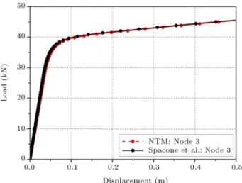
The load-displacement response at node 7 and the load-rotation response at node 9 obtained with the two models are compared in Figures 15 and 16,
Figure 9. Section moment vs. curvature for elements 1, 2, 3 and 4 in the cantilever system in Figure 6.
Figure 10. Simply supported beam system.
Figure 11. Load vs. displacement for node 3 in the simply supported beam system in Figure 10.
Figure 12. Load vs. rotation for node 5 in the simply supported beam system in Figure 10.
respectively. In general, there is good agreement be-tween the TTM model results and the results obtained with the exibility-based model. Small discrepancies between the two models are observed in the post-yielding responses due to ber section discretization. It is important to note that the proposed TMM model uses exact integration to derive the beam-section re-sponse, while the exibility-based model employs ber-section discretization to perform numerical ber-sectional integration. Figure 17 compares the sectional
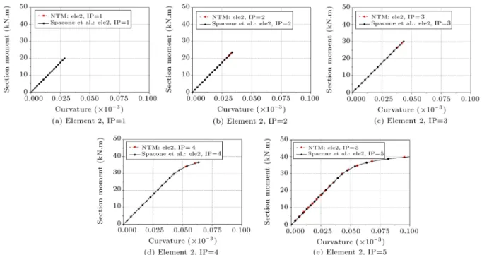
moment-Figure 13. Section moment vs. curvature at integration points of element 2 in the simply supported beam system in Figure 10.
Figure 14. Three-span continuous beam system.
Figure 15. Load vs. displacement for node 7 in the
Figure 17. Section moment vs. curvature at the last integration point of elements 3, 4, 7, and 8 for the 3-span continuous beam system in Figure 14.
curvature responses at the last integration point of elements 3, 4, 7, and 8. Clearly, the proposed TMM model is capable of representing the local response obtained with the exibility-based model.
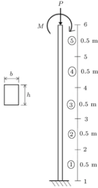
5.4. Cantilever column
A cantilever column of height H = 2:5 m is subjected to a constant axial load, P = 270 kN, and an incrementally increasing moment, M, at its free end, as shown in Figure 18. The column section is square with a dimension of b = H = 300 mm For the mechanical
Figure 18. Column system.
and strength properties of the beam, an initial elastic modulus of 20 GPa, a yield strength of 40 MPa, and a strain-hardening ratio of 0.01 are assumed. As shown in Figure 18, the column is discretized into ve proposed TMM elements. One exibility-based element is used to model this column. For the exibility-based model, 15 bers are used to discretize the column section, while, for the proposed TMM model, exact integration is employed to derive the column sectional response.
Figure 19 shows the tip load-displacement re-sponses obtained with the two models. Clearly, there is excellent agreement between the two models. Figure 20 compares the axial-moment interaction diagrams
con-Figure 19. Load vs. displacement for node 6 in the column system in Figure 18.
Figure 20. P-M interaction diagram for the column system in Figure 18.
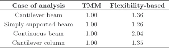
Table 1. Comparison of computational time ratio. Case of analysis TMM Flexibility-based
Cantilever beam 1.00 1.36 Simply supported beam 1.00 1.26 Continuous beam 1.00 2.04 Cantilever column 1.00 1.35
structed by the two models and indicates that they match quite perfectly.
The relative computational time of each analysis is shown in Table 1. The TMM model is a minimum of 1.26 times and a maximum of 2.04 times faster than the exibility-based frame model in simply supported beams and continuous beams, respectively.
6. Conclusion
In this study, a material-nonlinear-analysis algorithm based on the Transfer Matrix Method (TMM) is presented. This newly developed algorithm can be used to perform nonlinear analyses of continuous beam systems. In the TMM, the system equation has a constant number of system unknowns, regardless of the total degrees-of-freedom number in a structure and the system response (either linear or nonlinear). That is, the TMM model is at least 1.26 times faster than the exibility-based frame model in the analyses. As a result, TMM can be used eciently both for linear and nonlinear structural analyses. Four numerical studies conrm the accuracy and eciency of the proposed TMM model. In all examples, there is good agreement between the proposed TMM model and the exibility-based ber element model, both at global and local levels.
Acknowledgment
This research was supported by a grant (13SCIPA01) from the Smart Civil Infrastructure Research Program,
funded by the Ministry of Land, Infrastructure and Transport (MOLIT) of the Korean government and the Korean Agency for Infrastructure Technology Advance-ment (KAIA). Special thanks go to senior lecturer, Mr. Wiwat Sutiwipakorn, for reviewing and correcting the English of this paper.
References
1. Wilson, E.L. \The static condensation algorithm", Int. J. Numer. Method. Eng., 8(1), pp. 198-203 (1974). 2. McGuire, W. and Gallagher, R.H., Matrix Structural
Analysis, John Wiley & Sons Inc., New York (1979). 3. Cheung, Y.K., Finite Strip Method in Structural
Anal-ysis, Pergamon Press, Oxford (1976).
4. Pestel, E.C. and Leckie, F.A., Matrix Methods in Elastomechanics, McGraw-Hill, New York (1963). 5. Gimena, F.N., Gonzaga, P. and Gimena, L.
\Struc-tural matrices of a curved-beam element", Struct. Eng. Mech., 42(1), pp. 1-12 (2009).
6. Przemieniecki, J.S., Theory of Matrix Structural Anal-ysis, McGraw-Hill, New York (1968).
7. Ozturk, D., Bozdogan, K. and Nuhoglu, A. \Modied nite element-transfer matrix method for the static analysis of structures", Struct. Eng. Mech., 43(6), pp. 761-769 (2012).
8. Holzer, H., Die Berechnung der Drehschwingungen, Springer-Verlag, Berlin (1921).
9. Hetenyi, M., Beams on Elastic Foundations, University of Michigan Press, Ann Arbor, MI (1946).
10. Dokainish, M.A. \New approach for plate vibrations: Combination of transfer matrix and nite element technique", J. Eng. Ind. Trans. ASME., 94Ser B(2), pp. 526-530 (1972).
11. Chiatti, G. and Sestieri, A. \Analysis of static and dynamic structural problems by a combined nite element-transfer matrix method", J. Sound Vib., 67(1), pp. 35-42 (1979).
12. Sankar, S. and Hoa, S.V. \An extended transfer matrix-nite element method for free vibration pf plates", J. Sound Vib., 70(2), pp. 205-211 (1980). 13. Ohga, M. and Shigematsu, T. \Bending analysis of
plates with variable thickness by boundary element-transfer matrix method", Comput. Struct., 28(5), pp. 635-640 (1988).
14. Chen, Y. and Xue, H. \Dynamic large deection analysis of structures by a combined nite element-Riccati transfer matrix method on a microcomputer", Comput. Struct., 29(6), pp. 699-703 (1991).
15. Chen, Y. \Geometrically nonlinear dynamic analysis of plates by an improved nite element-transfer matrix method on a microcomputer", Struct. Eng. Mech., 2(4), pp. 395-402 (1994).
16. Akintilo, I. and Syngellakis, S. \Inelastic analysis of reinforced concrete coupled shear walls by the transfer matrix method", Struct. Eng., 67(15), pp. 284-288 (1989).
17. Rosignoli, M. \Reduced-transfer matrix method for analysis of launched bridges", ACI Struct. J., 96(4), pp. 603-608 (1999).
18. Pfeier, U. \Nonlinear analysis for plane reinforced or prestressed concrete frames taking into consideration axial elongation by cracking", Doctoral Thesis, Ham-burg University of Technology, Germany (2004). 19. Starossek, U., Lohning, T. and Schenk, J. \Nonlinear
analysis of reinforced concrete frames by a combined method", Electron. J. Struct. Eng., 9, pp. 29-36 (2009).
20. Spacone, E., Filippou, F.C. and Taucer, F.F. \Fibre beam-column model for non-linear analysis of R/C frames: Part I. formulation", Earthq. Eng. Struct. Dyn., 25(7), pp. 711-725 (1996).
21. Tonti, E. \The reason for analogies between physical theories", Appl. Math. Model., 1, pp. 37-50 (1977). 22. Chen, Z., The Finite Element Method: Its
Fundamen-tals and Applications in Engineering, World Scientic Publishing Co. Pte. Ltd., Singapore (2011).
23. Joe, H.Y., Nam, M.H., Kang, J.S. and Ha, D.H. \Sim-ple analysis of axisymmetrically loaded axisymmetrical shell by transfer matrix", Proceedings of 2th Asian-Pacic Conference on Computational Mechanics, Syd-ney, New South Wales, Australia (1993).
24. Jung, S.T. \An analysis of axisymmetrical circular plate by transfer matrix method", Doctoral Thesis, Gyeongsang National University, Korea (1995). 25. Manoharan, N. and Dasgupta, S.P. \Consolidation
analysis of elasto-plastic soil", Comput. Struct., 54(6), pp. 1005-1021 (1995).
26. Vecchio, F.J. \Nonlinear analysis of RC frames sub-jected to thermal and mechanical loads", ACI Struct. J., 84(6), pp. 492-501 (1987).
27. Yang, Y.B. and Kuo, S.R., Theory and Analysis of Nonlinear Framed Structures, Prentice-Hall, Singapore (1994).
28. Mazzoni, S., McKenna, F., Scott, M.H. and Fenves, G.L. et al., Open System for Earthquake Engineering Simulation (OpenSees), Version 1.7.3, Pacic Earth-quake Engineering Research Center, Berkeley, Califor-nia (2008).
Biographies
Minho Kwon is Professor of Structural Engineering in the Department of Civil Engineering at Gyeongsang National University, Jinju, South Korea. His main research interests include nite element modeling for RC and steel structures, aircraft crash analysis, earth-quake resisting design, constitutive modeling, and experimenting with RC structures under severe loads. He has conducted several research projects with the government and industry, and is member of the Amer-ican Society of Civil Engineers and the Korean Society of Civil Engineers.
Jinsup Kim received his PhD degree in Structural Engineering from the University of Gyeongsang Na-tional University, Jinju, South Korea, in 2014. His research interests include nite element analysis for RC and steel structures, and seismic reinforcing and retrotting for RC and steel structures using ber-reinforced polymer and high performance ber rein-forced concrete.
Hyunsu Seo is a PhD candidate in Civil Engineering from Gyeongsang National University, Jinju, South Korea. His major eld of interest is structural engineer-ing and numerical modelengineer-ing of civil structures. He is also interested in numerical simulation of experimental modeling in reinforced concrete and steel frame struc-tures. He is currently involved in several national R&D projects.
Suchart Limkatanyu is Associate Professor in the Department of Civil Engineering at the Prince of Songkla University, Thailand. He received his PhD degree in Structural Engineering and Structural Me-chanics (SESM) from the University of Colorado, Boulder, USA. His research interests center on the seismic analysis, design and retrotting of reinforced concrete structures, earthquake engineering, compu-tational mechanics, nonlinear frame analysis, nano-engineering and technology, and multi-physics sys-tems.