ISSN: 2252-8938, DOI: 10.11591/ijai.v9.i3.pp417-423 417
Long-term load forecasting using grey wolf optimizer
-least-squares support vector machine
Z. M. Yasin1, N. A. Salim2, N.F.A. Aziz3, Y.M. Ali4, H. Mohamad51,2,4,5Faculty of Electrical Engineering, Universiti Teknologi MARA, Malaysia 3Faculty of Electrical Engineering, Universiti Tenaga Nasional, Malaysia
Article Info ABSTRACT
Article history: Received Feb 27, 2020 Revised Apr 20, 2020 Accepted May 17, 2020
Long term load forecasting data is important for grid expansion and power system operation. Besides, it also important to ensure the generation capacity meet electricity demand at all times. In this paper, Least-Square Support Vector Machine (LSSVM) is used to predict the long-term load demand. Four inputs are considered which are peak load demand, ambient temperature, humidity and wind speed. Total load demand is set as the output of prediction in LSSVM. In order to improve the accuracy of the LSSVM, Grey Wolf Optimizer (GWO) is hybridized to obtain the optimal parameters of LSSVM namely GWO-LSSVM. Mean Absolute Percentage Error (MAPE) is used as the quantify measurement of the prediction model. The objective of the optimization is to minimize the value of MAPE. The performance of GWO-LSSVM is compared with other methods such as LSSVM and Ant Lion Optimizer – Least-Square Support Vector Machine (ALO-LSSVM). From the results obtained, it can be concluded that GWO-LSSVM provide lower MAPE value which is 0.13% as compared to other methods.
Keywords:
Grey wolf optimizer Load forecasting LSSVM
This is an open access article under the CC BY-SA license.
Corresponding Author: Zuhaila Mat Yasin,
Faculty of Electrical Engineering, Universiti Teknologi MARA,
40450 Shah Alam, Selangor, Malaysia. Email: [email protected]
1. INTRODUCTION
Planning in power systems is a projection of how the system should evolve over a specific time-frame. It has become more difficult to plan power systems in developing countries. Planning must be completed despite numerous vulnerabilities such as future load designs, population growth and economic growth representing developing countries, technical, economic and environmental constraints [1]. Load forecasting plays an important role in planning power systems to ensure uninterrupted and economical power generation and distribution to consumers. Precise electrical load forecasting is a major issue in the planning and management of electricity generating utilities.
The load forecast can be divided into three classifications. Short-term load forecasting (STLF) covers an hour to a week time [2]. Short term load forecasting contributes to the decision-making process, including unit commitment and process for improving security [3]. The accurate load forecasting helps enhancing the unit commitment scheduling and thus can save large amount of cost per year [4]. Medium load forecasting (MTLF) covers a week-to-year period. It is essential for fuel supply and maintenance operations to be planned [5]. Long-term load forecast (LTLF) forecast for more than one year [6]. Long term load forecasting facilitates the decision-making of an electrical utility including
the purchase and generation of electricity, load switching and infrastructure development. The importance of load prediction turns out to be more noteworthy in high-growth developing countries. Understanding and forecasting of load characteristics was complex due to its dependence on a wide range of factors influencing the weather, geographical diversity, sunrise/sunset time, seasonal diversity, etc. [7]. Despite the increase in electricity demand annually, the pattern of the load profile may also change [8-9].
Analysis of long-term load forecasting has received little attention. Reference [10] presented a long term load forecast using Fuzzy Logic model. Fuzzy logic model was developed based on the weather parameters which are temperature and humidity. Two years historical load data were utilized to predict a year-ahead load demand. The value of Mean Average Percentage Error (MAPE) obtained was 6.9%. The technique is then improved in [11] using Fuzzy-Neuro. Fuzzy-Neuro is the combination of Fuzzy Logic and Artificial Neural Network (ANN). In Fuzzy-Neuro, the output of the fuzzy logic system are fed to ANN. Fuzzy logic systems used for making decision based on the rules, meanwhile, ANN is used for training and testing process. The characteristic of ANN are high learning capabilities, adaptability and generalization. By using Fuzzy-Neuro, MAPE has improved to 1.22%.
Recently, various Artificial Intelligent (AI) techniques can be implemented for forecasting. One of them is ANN. Research in ANN has received considerable attention. ANN has many advantages as compared to the conventional computational systems such as computation speed and robustness. The most profound and important characteristic of ANN is the ability to memorize which involves a large number of processors operating in parallel. Each processors consists of own knowledge and can access the data in its local memory. The ability of ANN to generalize on unseen data and learn from noisy data make it a very powerful machine learning algorithm [12]. Apart from ANN, there is another intelligent system that has been given attention recently namely Support Vector Machine (SVM). The advantages of SVM including fast convergence rate, good generalization capability and automatic determination of hidden neurons [13]. The regression problem in SVM is formulated based on convex quadratic programming problem where it use linear regressor [14]. In linear regressor, the regressor will maps the inputs into a higher dimensional feature space to minimize the cost function. The major shortcoming of SVM is the computational burden for optimization programming constrained. This weakness has been overcomed in Least-Square Support Vector Machines (LSSVM), which substitute a quadratic programming with linear equations [15-18]. The accuracy of the prediction of LSSVM depends on the hyperparameters value setting. Therefore, Grey Wolf Optimizer - Least Square Support Vector Machine(GWO-LSSVM) is proposed to solve long-term load forecasting problem. GWO is integrated with LSSVM for determining the optimal hyperparameters. GWO is inspired by hierarchy system and hunting mechanism of grey wolves in nature. GWO has been effectively implemented for solving various power system problems [19-23].
2. RESEARCH METHOD
In order to predict total load demand, a total of 1035 sets of data are collected in the area of Dayton, Ohio, US from January 2016 until May 2018. For training, 668 data sets are used and the remaining 367 data sets are used for testing. Moreover, the temperature, wind speed and humidity are the inputs, while the total output power is the output of the model. Figure 1 presents overall data used in this paper. It can be observed that the total load demand fluctuated. Therefore, an accurate prediction technique is required to ensure the electricity generated capacity meet electricity demand at all times. In this paper, GWO-LSSVM is developed to predict the total load demand in long-term duration. The efficacy of the proposed algorithm is evaluated through comparison with other techniques such as LSSVM and Ant Lion Optimizer- Least-Square Support Vector Machine (ALO-LSSVM).
2.1. Prediction measurement
Mean Absolute Percentage Error (MAPE) and coefficient of determination (R2) were used for the
evaluation purposes as shown in (1) and (2). Both of them act as indicators which assess the performance of suggested technique. MAPE is a measure of prediction precision of a forecasting technique in measurements. It usually uses percentage to shows the accuracy. For MAPE, the lower the value, the better the performance. In the simulation, MAPE is utilized as objective function of GWO-LSSVM. The coefficient of determination, R2 is a part of the output variable variance that can be predicted from the input variable. It gives a measure of
how similar the outcomes are replicated by the model, in view of the extent of total variation of results clarified by the model. However, for R2, the closer the value to 1, the better it will be.
𝑀𝐴𝑃𝐸 = ∑ |𝐹𝑡−𝐴𝑡| |𝐹𝑡| 𝑛
𝑡=1 × 100% (1)
𝑅2= 1 −∑(𝐴𝑡−𝐹𝑡)2
∑(𝐴𝑡−𝐴̅𝑡)2 (2)
Where t=1, 2, …., t At = Actual values
Ft = Predicted values/Forecasting values
2.2. Development of GWO-LSSVM
GWO is a metaheurictic-based technique stimulated by the hunting behavior and leadership hierarchy of grey wolves as depicted in Figure 2. Alpha (α) is the leader of the wolves. It is responsible to make a settlement which are relates to hunting, when and where to sleep, and etc [24]. Beta (β) is the second level which is the assistant of α in making decision. β is likewise the best applicant to replace α when α getting old or die. The lowest in grey wolves’ system hierarchy is called Omega (ω). It acts as a scapegoat. ω can fulfill the entire whole grey wolves group. The third level in grey wolves’ system hierarchy is Delta (δ) which must report to α and β, however they lead the ω. δ responsibility is scouting to secure and ensure the security of the group of wolves. The system hierarchy of grey wolves is an assigned characteristic used in GWO. Another amazing characteristic of wolves is the group hunting strategy. The fittest solution is considered as the α. Meanwhile, the second and third best solutions are considered as β and delta δ respectively. The rest of the individual solutions are considered as ω. During hunting, the wolves tend to encircle their prey. The encircling behaviour is represented as (3).
𝐷⃗⃗ = |𝐶 . 𝑋⃗⃗⃗⃗ − 𝑋 (𝑡)𝑝
𝑋 (𝑡 + 1) = 𝑋⃗⃗⃗⃗ (𝑡) − 𝐴 . 𝐷𝑝 ⃗⃗ (3)
𝐴 = 2𝑎⃗ . 𝑟⃗⃗⃗ − 𝑎 1
𝐶 = 2. 𝑟⃗⃗⃗ 2
Where t is the ongoing iteration
𝐴 and 𝐶 are coefficient vectors
𝑋𝑝
⃗⃗⃗⃗ is the position vector of the prey
𝑋𝛼, 𝑋𝛽, and 𝑋𝛿 is the position of the search agent. The best three solutions; 𝑋𝛼, 𝑋𝛽, and 𝑋𝛿 are saved including the latest positions of ω according to the current best position. 𝑋𝛼 is the best position of α, 𝑋𝛽 is the best position of β, and 𝑋𝛿 is the best position of δ. The final position X(t+1), is defined by the positions of α, β, and δ in the search space as shown in (4).
𝑋 is the position of the grey wolf
𝐷𝛼
⃗⃗⃗⃗⃗ = |𝐶⃗⃗⃗⃗ . 𝑋1 ⃗⃗⃗⃗ − 𝑋 |𝛼
𝐷𝛿
⃗⃗⃗⃗ = |𝐶⃗⃗⃗⃗ . 𝑋3 ⃗⃗⃗⃗ − 𝑋 |𝛿
𝑋1
⃗⃗⃗⃗ = 𝑋⃗⃗⃗⃗ − 𝐴𝛼 ⃗⃗⃗⃗ . (𝐷1 ⃗⃗⃗⃗⃗ )𝛼 (4)
𝑋2
⃗⃗⃗⃗ = 𝑋⃗⃗⃗⃗ − 𝐴𝛽 ⃗⃗⃗⃗ . (𝐷2 ⃗⃗⃗⃗ )𝛽
𝑋3
⃗⃗⃗⃗ = 𝑋⃗⃗⃗⃗ − 𝐴𝛿 ⃗⃗⃗⃗ . (𝐷3 ⃗⃗⃗⃗ )𝛿
𝑋 (𝑡 + 1) =𝑋⃗⃗⃗⃗⃗ +𝑋1 ⃗⃗⃗⃗⃗ +𝑋2 ⃗⃗⃗⃗⃗ 3 3
Where 𝐷⃗⃗ is the coefficient vector
In LSSVM, there are two tuning parameters that associated with RBF kernel, σ2 and
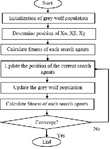
regularization parameter, γ. These parameters affect the LSSVM estimation model's accuracy. These parameters are optimized using GWO-LSSVM to minimize MAPE. The flowchart of GWO-LSSVM is presented in Figure 3.
Figure 2. The system hierarchy of grey wolves
Figure 3. Flowchart of GWO-LSSVM
During initialization, two parameters which are gamma and sigma were randomly generated within lower bound and upper bound. The parameters set for GWO-LSSVM algorithm are tabulated in Table 1. The number of search agents is set to 10. If the number of search agents is high, it will consume more time. However, small number of search agents may not give the best prediction.
Table 1. Parameters of GWO
Parameter Value
Number of search agents 10
Maximum iteration 30
Upper bound 1000000
Lower bound 0.1
The position of grey wolf is then updated according to (4). α, β, and δ wolves determine the possible position of the prey. This process continue until the convergence goal is met and 𝑋𝛼 is taken as the best solution. In this algorithm, MAPE is set as the fitness function. MAPE value is obtained by calling the LSSVM algorithm. The position of search agents are updated according to α, β, and δ in search space as shown in (4). The process is repeated until the solution converged. The solution will converge if the different between maximum and minimum fitness reach 1x10⁻⁷. In this paper, the results of GWO-LSSVM is also
compared to ALO-LSSVM in terms of accuracy and convergence speed. In ALO-LSSVM, ALO is utilized to determine the optimal parameters of gamma and sigma. The algorithm represents the hunting behavior of antlions in nature. There are five main steps of the algorithm including random walk of ants, constructing traps, entrapment of ants in traps built by antlions, catching ants, and re-setup the traps [25]. The number of serach agents, maximum iterations, lower and upper bound are set similar with GWO-LSSVM.
3. RESULTS AND DISCUSSION
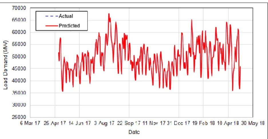
Figure 4 presents the results of GWO-LSSVM for training data. The red line is defined as the estimation or predicted output, while the blue dots represented as the actual output. The optimal gamma and sigma value are 106784.335 and 0.85381 respectively. The comparison between predicted and actual data for
training and testing process using GWO-LSSVM are shown in Figure 5 and Figure 6 respectively. It can be observed that the predicted results almost similar with actual data for both training and testing process.
Figure 4. Results of GWO-LSSVM
Figure 5. Comparison of training data and estimation output for GWO-LSSVM
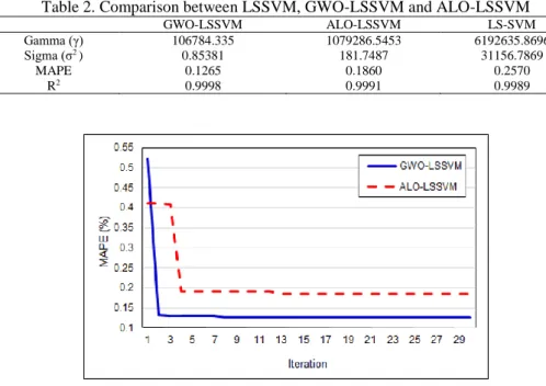
Comparison between GWO-LSSVM, ALO-LSSVM and LSSVM is tabulated in Table 2. By running GWO-LSSVM, the values of optimal parameters of γ and σ2 are 106784.335 and 0.85381 respectively. As the maximum number of iterations reaches 30, MAPE and R2 are compared.
By using LSSVM to model the total output power, the values of MAPE was 0.2570%. However, by using ALO-LSSVM, it helps in reducing the MAPE values to 0.1860%. For GWO-LSSVM, the MAPE is much better than the other two methods which is 0.1265%. For the coefficient of determination, R2, LSSVM gives
the value of 0.9989. However, the optimal values of parameters γ and σ2 by using hybrid techniques GWO-LSSVM and ALO-LSSVM, the R2 increased to 0.9998 and 0.9991 respectively. Thus, it can be
concluded that GWO-LSSVM provide more accurate prediction for long-term load forecasting as compared to other techniques. The comparison of iterative convergence between GWO-LSSVM and ALO-LSSVM is presented in Figure 7. GWO-LSSVM converged at 7th iteration while ALO-LSSVM
converged at 12th iteration. It can be concluded that GWO-LSSVM has a precise prediction and the speed of
optimization is faster.
Table 2. Comparison between LSSVM, GWO-LSSVM and ALO-LSSVM
GWO-LSSVM ALO-LSSVM LS-SVM
Gamma (γ) 106784.335 1079286.5453 6192635.8696
Sigma (σ2 ) 0.85381 181.7487 31156.7869
MAPE 0.1265 0.1860 0.2570
R2 0.9998 0.9991 0.9989
Figure 7. Convergence graph for GWO-LSSVM and ALO-LSSVM
4. CONCLUSION
A hybrid prediction technique namely Grey Wolf Optimizer – Least Square Support Vector Machine (GWO-LSSVM) had been develop to forecast long-term load demand, with the objective function to minimize the error. LSSVM is one of the good techniques to solve nonlinear problems. However, the accuracy of the prediction depends on the selection of the RBF parameters. GWO has been utilized to optimized the value of these parameters. GWO mimics the hierarchy of leadership and hunting mechanism of grey wolf in nature. Four inputs were considered for the prediction; peak load demand, temperature, humidity and wind speed. After conducting the simulation for LSSVM, GWO-LSSVM and ALO-LSSVM, it can be concluded that GWO-LSSVM has better prediction accuracy and higher optimization speed to predict the long-term load forecasting as it.
ACKNOWLEDGEMENTS
This research is fully supported by Universiti Teknologi MARA Malaysia and the Ministry of Higher Education (MOHE) Malaysia through research grant 600-IRMI/FRGS 5/3 (157/2019).
REFERENCES
[1] A. M. Al-Shaalan, “Essential aspects of power system planning in developing countries,” Jurnal of King Saud University, vol. 23, no. 1, pp. 27-32, 2011.
[2] Zizi Zhang, Hong Li, Yang Zhao, and Xiaobo Hu, “Short-term load forecasting based on the grid method and the time series fuzzy load forecasting method,” in Int.Conference on Renewable Power Generation (RPG 2015), 2015. [3] T. Hong and S. Fan, “Probabilistic electric load forecasting: A tutorial review,” Int. Journal of Forecast., vol. 32,
no. 3, pp. 914-938, 2016.
[4] T. Saksornchai, W. J. Lee, K. Methaprayoon, J. R. Liao, and R. J. Ross, “Improve the unit commitment scheduling by using the neural-network-based short-term load forecasting,” IEEE Trans. Industrial Applications, vol 41, no. 1, pp: 169-179, 2005.
[5] S. Wang, S. Wang, D. Wang,"Combined probability density model for medium term load forecasting based on quantile regression and kernel density estimation", in Energy Procedia, vol. 158, no. 1, pp. 6446-6451, 2019. [6] J. Moral-Carcedo and J. Pérez-García, “Integrating long-term economic scenarios into peak load forecasting: An
application to Spain,” Energy, vol. 140, no. 1, pp. 682-695, 2017.
[7] S. M. Badran, “Neural network integrated with regression methods to forecast electrical load,” in IET Int. Conference on Developments in Power Systems Protection, 2012.
[8] K. B. Lindberg, P. Seljom, H. Madsen, D. Fischer, and M. Korpås, “Long-term electricity load forecasting: Current and future trends,” Utilities Policy, vol. 58, no. 1, pp. 102-119, 2019.
[9] K. Khalid, A. Mohamed, R. Mohamed, H. Shareef, "Performance comparison of Artificial Intelligence techniques for non-intrusive electric load monitoring", in Bulletin of Electrical Engineering and Informatics, vol. 7, no. 2, pp. 143-152, 2018.
[10] D. Ali, M. Yohanna, M. I. Puwu, and B. M. Garkida, “Long-term load forecast modelling using a fuzzy logic approach,” in Pacific Science Review A: Natural Science and Engineering, vol. 18, no. 2, pp. 123-127, 2016. [11] D. Ali, M. Yohanna, P. M. Ijasini, and M. B. Garkida, “Application of fuzzy – Neuro to model weather parameter
variability impacts on electrical load based on long-term forecasting,” Alexandria Engineering Journal, vol.57, no. 1, 2018.
[12] C. T. Hsu, M. S. Kang and C. S. Chen, "Design of Adaptive Lopad Shedding by Artificial Neural Networks," IEE Proc. of Generation, Transmission and Distribution, vol. 152, pp. 415-421, May 2005.
[13] M. Nizam, A. Mohamed, M. Al-Dabbagh and A. Hussain, "Using Support vector Machines for Determining Voltage Unstable Areas in Power Systems," 2nd Int. Conference on Power and Energy Conference (PECon2008), pp. 878-883, 2008.
[14] N.S. A. Yasmin, N.A. Wahab, A.N. Anuar, M. Bob, "Performance comparison of SVM and ANN for aerobic granular sludge", in Bulletin of Electrical Engineering and Informatics, vol. 8, no. 4, pp. 1392-1401, 2019.
[15] C. Liu, L.Tang, J. Liu, “Least Squares Support Vector Machine with self-organizing multiple kernel learning and sparsity”, in Neurocomputing, vol. 331, no. 1, pp. 493-504, 2019.
[16] L. Kumar, S.K. Sripada, A. Sureka, S.K. Rath, “Effective fault prediction model developed using Least Square Support Vector Machine (LSSVM)”, in Journal of Systems and Software, vol. 13, no. 1, pp. 686-712, 2018. [17] A. Yang, W. Li, X. Yang, "Short-term electricity load forecasting based on feature selection and Least Square
Support Vector Machines", in Knowledge-Based Systems, vol. 16, no. 1, pp. 159-173, 2019.
[18] M. A. A. Aziz, Z. M. Yasin, and Z. Zakaria, “Prediction of photovoltaic system output using hybrid least square support vector machine,” in 7th IEEE International Conference on System Engineering and Technology, pp. 1-7, 2017.
[18] T. Jayabarathi, T. Raghunathan, B. R. Adarsh, and P. N. Suganthan, “Economic dispatch using hybrid grey wolf optimizer,” Energy, vol. 111, pp. 630-641, 2016.
[19] S. Mohanty, B. Subudhi, and P. K. Ray, “A new MPPT design using grey wolf optimization technique for photovoltaic system under partial shading conditions,” IEEE Trans. Sustainability Energy, vol. 7, no. 1, pp. 181-188, 2016.
[20] U. Sultana, A. B. Khairuddin, A. S. Mokhtar, N. Zareen, and B. Sultana, “Grey wolf optimizer based placement and sizing of multiple distributed generation in the distribution system,” Energy, vol. 111, no. 1, pp. 525-536, 2016. [21] A. Lakum and V. Mahajan, “Optimal placement and sizing of multiple active power filters in radial distribution
system using grey wolf optimizer in presence of nonlinear distributed generation,” Electric Power System Research, vol. 173, no. 1, pp. 281-290, 2019.
[22] M.Z.M. Tumari, M.H. Suid, M.A. Ahmad, “PV system reactive power coordination with ULTC & shunt capacitors using grey wolf optimizer algorithm”, in Indonesian Journal of Electrical Engineering and Computer Science, vol. 19, no. 1, pp. 1-10, 2020.
[23] C. Muro, R. Escobedo, L. Spector, and R. P. Coppinger, “Wolf-pack (Canis lupus) hunting strategies emerge from simple rules in computational simulations,” Behavioural Processes, vol. 88, no. 3, pp. 192-197, 2011.
[24] S. Mirjalili, S. M. Mirjalili, and A. Lewis, “Grey Wolf Optimizer,” Advances in Engineering Software, vol. 69, pp. 46-61, 2014.
[25] I. N. Sam’on, Z. M. Yasin, Z. Zakaria, “Ant Lion Optimizer for Solving Unit Commitment Problem in Smart Grid System”, Indonesian Journal of Electrical Engineering and Computer Science, vol. 8, no. 1, pp. 129-136, 2017.