196
A stochastic bi-objective multi-product programming model to
supply chain network design under disruption risks
Fatemeh Sabouhi
1, Mohammad Saeed Jabalameli
1*1School of Industrial Engineering, Iran University of Science and Technology, Tehran, Iran
[email protected], [email protected]
Abstract
Emphasize on cost-cutting, increasing customers' satisfaction, and trying to manage and reduce the risks are among the key strategies of decision-makers in the design of supply chain networks. This study provides a stochastic bi-objective multi-product optimization model for designing a resilient supply chain network under disruption risks. The objectives of the proposed model are minimizing the total cost of the supply chain, as well as, minimizing the non-resiliency of the network. In addition, a ε-constraint method is used to convert the bi-objective model into a single-objective formulation. The model decisions include locating manufacturers, warehouses, and distribution centers and determining the amount of production of different products in each manufacturer, the amount of product transport between the different nodes of the network, and the amount of lost sales for different products in each market. The validity of the proposed model is investigated through random examples and the results of the model implementation on these examples are presented.
Keywords: bi-objective optimization model, supply chain network design, resilience, disruption risks
1- Introduction
1-1- Motivation
A supply chain comprises of all organizations involved (either directly or indirectly) in the processes of producing, providing customer service, and meeting the needs of suppliers, manufacturers, shipping companies, warehouses, and distributor centers (Papapostolou et al., 2011). Therefore, supply chain management refers to the effective management of information, financial and material flows between the chain members with the purpose of maximizing the total profit and customer satisfaction (Sabouhi et al., 2018b).
The modern and competitive global economy has developed complex and interconnected supply chains for the benefits that companies achieve in complex processes and strategies, such as access to skilled labor and cheap raw materials, globalization, outsourcing, timely production and delivery, and lean practices (Hasani and Khosrojerdi, 2016, Vaez, 2017, Vaez et al., 2018). While these measures in most supply chains result in cost-cutting and increasing the quality and flexibility, achieving these benefits also leads to some risks for the supply chains (Tang, 2006b). As supply chains become more complex, they become more vulnerable to the risks created by different sources. The risks that threaten supply chains and can greatly affect their performance are the existing uncertainties in the environment, including uncertainties in supply, demand, and costs and disruptions caused by natural and man-made disasters such as floods, earthquakes, storms, political unrest, strikes, and terrorist activities (Scheibe and Blackhurst, 2018, Ghavamifar and Sabouhi, 2018, Sabouhi et al., 2018a).
*Corresponding author
ISSN: 1735-8272, Copyright c 2019 JISE. All rights reserved
Journal of Industrial and Systems Engineering
Vol. 12, No. 3, pp. 196-209 Summer (July) 2019
197
There are many studies in the literature of supply chain network design under uncertainty. For example, we can refer to the models developed by Santoso et al. (2005), Baghalian et al. (2013), Cardoso et al. (2015), Han et al. (2015), Yin et al. (2015), Giri and Bardhan (2015), Jabbarzadeh et al. (2014), Zokaee et al. (2017), and Sabouhi et al. (2019). Disruption risks can make more significant economic and social damages than the existing uncertainties in the environment. Thus, lack of identification and appropriate management of such risks in long-term can result in negative effects such as distrust, increased dissatisfaction, pessimism towards companies, excessive price increases due to lack of goods, stock depreciation, increased delivery times, and delay in the provision of services (Sabouhi et al., 2016). Thus, supply chains must identify, evaluate and rank the disruption risks and take the necessary measures to manage them in order to remain in the competitive environment and achieve their goals (Nishat Faisal et al., 2006).
Considering what was mentioned earlier, the design and planning of supply chains in a resilient way that can act against disturbances are of great importance (Schütz and Tomasgard, 2011). The resilient supply chain can be defined as the ability of a chain to return to its original state or a new state (a more favorable state than its disorder state) (Bhamra et al., 2011). On the other hand, how to deal with disruption risks is very dependent on the design and structure of the supply chain. In other words, well-designed supply chains are able to provide a more appropriate response to random disruptions (Dixit et al., 2016). Hence, the design of the resilient supply chain network has attracted the attention of many researchers (Jabbarzadeh et al., 2018).
This paper aims to address the following questions. How could we measure resiliency of a network in supply chain design models? How could we analyze the conflicts between total cost and non-resiliency of the network? What are the impacts of changes in facilities' capacity on the total cost?We utilized random examples to investigate responses to these questions.
1-2- Literature review
The model efforts in the area of resilient supply chain network design have mostly focused on investigating different strategies to reduce the negative impacts of disruptions risks. These strategies are such as multiple sourcing, facility fortification, contracting with backup facilities, and maintaining the pre-positioned emergency inventory. For instance, Peng et al. (2011) proposed a network of suppliers and customers under disruption risks and used multiple sourcing strategy to deal with these risks. The aim of their model was to locate suppliers and determine the flow of products from suppliers to customers. Li and Savachkin (2013) developed a location model for a network of facilities and customers with complete and partial disruptions. In their proposed model, facility fortification and contracting with backup facilities strategies are used to increase the level of supply chain resiliency. Azad et al. (2013) presented a resilient supply chain network under the disruption of distribution centers and shipping links. They used the fortification of distribution centers and backup shipping to reduce the disruption risks.
Nooraie and Parast (2016) designed a supply chain network including suppliers, manufacturers, warehouses, distributors and customers. They proposed a multi-objective multi-product multi-periodic stochastic model under the partial disruption of facilities and used multiple sourcing to improve the resilience level of the supply chain. The objectives of their model were minimizing total costs and maximizing revenue from opening up facilities and selling products. Garcia-Herreros et al. (2014) developed a two-stage stochastic model under disruptions. In this model, additional inventory holding at distribution centers was used as a resilience strategy. Farahani et al. (2017) presented a multi-product model for locating facilities, and utilized the substitutable multi-product strategy to deal with partial disruption of facilities.
All of the studies mentioned here have only used resilience strategies to cope with disruption risks. However, most companies are trying to maximize network resiliency with least cost. Although the measurement of network resiliency is a new field in literature, several indicators based on network structure are introduced to address this issue. These indicators are such as the node criticality, the node complexity, and the flow complexity. The only works carried on in this regard are the models developed by Chopra and Sodhi (2004) and Zahiri et al. (2017).
The research gaps are identified as follows. First, the design of a multi-echelon supply chain network under production disruptions have not been widely discussed in the literature of resilient supply chain. Second, only few studies have addressed measures such as the node criticality, the node
198
complexity, and the flow complexity to measure resiliency of the network. Third, most of the existing works do not consider conflicts between multiple delivery goals to design a resilient supply chain network against major disruptions.
Given the above-mentioned challenges, the present study contributes to this area by presenting a stochastic bi-objective multi-product programming model to design a resilient supply chain network under production disruptions. In addition to multiple sourcing strategy, node criticality, node complexity, and flow complexity criteria are used to measure the network resiliency level. The objectives of the proposed model include minimizing the total cost of the supply chain and minimizing the non-resiliency of the network. The model decisions include locating manufacturers, warehouses, and distribution centers, as well as determining the amount of production of different products in each manufacturer, the amount of product transport between the different nodes of the network, and the amount of lost sales for different products in each market.
This study is organized as follows: First, the problem under investigation and the mathematical modeling are presented. Then, the results of the model solution on random examples are reported and the conclusions are provided.
2- Problem statement
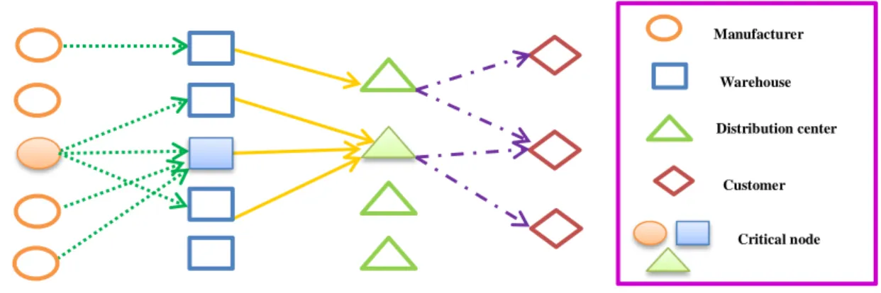
According to figure 1, a four-level network consisting of manufacturers, warehouses, distribution centers, and markets is considered. All the products after production at the manufacturers are sent to warehouses for storage. Then, the products are delivered to the markets through distribution centers. Disruption is one of the most important threats to supply chain performance. We assume that the capacity of manufacturers for the production of final products is vulnerable to disruptive risks. The possibility of partial and complete disruption of manufacturers is considered and a set of scenarios are defined to show situations in which one or more manufacturers are impacted by disruptions. In addition, the measures of node criticality, node complexity, and flow complexity, and multiple sourcing strategies are used to increase the reliability of the entire network against disruptions. The model decisions include locating manufacturers, warehouses, and distribution centers and determining the amount of production of different products in each manufacturer, the amount of product transport between the different nodes of the network, and the amount of lost sales for different products in each market.
In order to determine the above decisions, a stochastic bi-objective multi-product programming model is proposed for the design of a resilient supply chain network. The first objective function minimizes the total expected cost of the supply chain, while the second objective function minimizes the non-resiliency of the network. The ε-constraint method is used to convert the proposed model into a single-objective model.
The model assumptions are as follows:
1. The potential locations for opening of manufacturers, warehouses, and distribution centers are known.
2. Manufacturers, warehouses, and distribution centers have limited capacity.
3. Each random scenario occurs independently and with a certain probability of occurrence. 4. The problem is programmed for several products.
Fig 1. The structure of the supply chain network under investigation
Manufacturer
Warehouse
Distribution center
Customer
199
3- Model description
The following sets, parameters, and decision variables are introduced.
Sets
Set of potential locations for opening of manufacturers (i I )
I
Set of potential locations for opening of warehouses ( jJ )
J
Set of potential locations for opening of distribution centers (mM )
M
Set of markets (k K )
K
Set of products (
n
N
)N
Set of disruption scenarios (
s
S
)S
Parameters
Unit transportation cost from manufacturer i to warehouse j
ij
c
Unit transportation cost from warehouse j to distribution center m
jm
c
Unit transportation cost from distribution center mto marketk
mk
c
Cost of opening manufacturer i
i
f
Cost of opening warehouse j
j
f
Cost of opening distribution center m
m
f
Unit production cost of product n at manufacturer i
ni
p
Maximum production capacity of manufacturer i
i
e
Maximum capacity of warehouse j
j
a
Maximum capacity of distribution centerm
m
b
Unit cost of lost sales for product n at marketk
nk
g
Demand for product n at market k
kt
d
Percentage of lost capacity of manufacturer i under scenarios
is
Occurrence possibility of scenario s
s
Penalty coefficient for critical manufacturers
Penalty coefficient for critical warehouses
Penalty coefficient for distribution centers
Penalty coefficient for flow complexity between nodes j andi
Penalty coefficient for flow complexity between nodes m and j
200
Penalty coefficient for flow complexity between nodes k andm
Penalty coefficient for node complexity of manufacturers
Penalty coefficient for node complexity of warehouses
Penalty coefficient for node complexity of distribution centers
Variables
Equal to 1 if manufacturer i is opened; 0, otherwise
i
W
Equal to 1 if warehouses j is opened; 0, otherwise
j
Y
Equal to 1 if distribution center mis opened; 0, otherwise
m
T
Equal to 1 if manufacturer i is allocated to warehouses j ; 0, otherwise
ij
u
Equal to 1 if warehouses j is allocated to distribution center m ; 0, otherwise
jm
v
Equal to 1 if distribution center mis allocated to market k ; 0, otherwise
mk
h
Production amount of product n by manufacturer i under scenario s
nis
O
Amount of product n shipped from manufacturer i to warehouses j under scenario
s
nijs
X
Amount of product n shipped from warehouses j to distribution center m under scenario s
njms
Q
Amount of product n shipped from distribution center m to market k under scenario s
nmks
R
Amount of lost sales for product n at market k under scenario s
nks
G
3-1- Resiliency measures
Node criticality
A critical node is referred to a condition where the total input and output flows to that node are higher than a certain threshold. This strategy shows the total number of critical nodes in a supply chain. Therefore, as the number of critical nodes in a supply chain increases, its resiliency decreases (Zahiri et al., 2017, Cardoso et al., 2015). Equations (1)-(5) represent the critical nodes for manufacturers, warehouses, and distribution centers, respectively.
(1)
,i s
1
i nis nijs i
n n j
W
O
X
l
(2)
,j s
1
j njms nijs j
n m n i
Y
Q
X
l
(3)
,m s
1
m njms nmks m
n j n k
201
(4)
, , , , ,i j m k n s
, , , 0
nis nijs njms nmks
O X Q R
(5)
, ,i j m
, , {0,1}
i j m
W Y T
Flow complexity
The flow complexity measures the total interaction between the supply chain nodes. The increase of supply chain complexity makes the difficulty of its management and accordingly leads to a reduction in effective responsiveness to disruptions. In other words, the increase of complexity means increasing the number of nodes and their relationship, which results in increasing the occurrence possibility of disruptions and the recovery time of supply chain. Such disruptions ultimately cause high losses and negative impacts on firms' performance (Chopra and Sodhi, 2004, Hendricks et al., 2009, Tang, 2006a, Tang, 2006b). According to this measure, if the total number of related links would be high, the total flow in the network is complex. Equations (6) and (7) represent the total number of network links.
(6)
ij jm mk
i j i j m k
u
v
h
(7)
, , ,i j m k
, , {0,1}
ij jm mk
u v h
Node complexity
The node complexity indicates the total number of nodes in a network. Based on this measure, if the total number of active nodes in a network would be high, the network has a node complexity. Equations (8) and (9) show the total number of opened facilities in the network.
(8)
i j m
i j m
W
Y
T
(9)
, , ,i j m k
, , {0,1}
i j m
W Y T
3-2- Mathematical modeling
This section introduces a new linear programming model to design a resilient supply chain. To formulate the problem under investigation, a two-stage stochastic programming approach (see Birge and Louveaux (2011)) is used. In this approach, there are two types of decisions: first-stage and second-stage decisions. The first-stage decisions are determined before realizing disruption scenarios and consist of locating manufacturers, warehouses, and distribution centers while the second-stage decisions are related to specific disruption scenarios and include determining the amount of production of different products in each manufacturer, the amount of product transport between the different nodes of the network, and the amount of lost sales for different products in each market.
(10)
1 (
)
i i j j m m s ni nis ij nijs
i j m s n i n i j
jm njms mk nmks nk nks
n i j n i j n k
Min Z f W f Y f T p O c X
c Q c R g G
202
(11)
2 i j m ij jm mk
i j m i j i j m k
i j m
i j m
Min Z W Y T u v h
W Y T
(12) , i s (1
)
nijs is i i
n
X
e W
(13)
,
j s
njms j j n m
Q
a Y
(14)
,
k s
nmks m m n m
R
b T
(15)
, ,
i n s
nis nijs j
O
X(16)
, ,
j n s
nijs njms
i m
X
Q
(17)
, ,
m n s
njms nmks
j k
Q R
(18)
, ,
k n s
nmks nks nk m
R
G
d
(19)
, ,
i j s
nijs ij i n
X
u e
(20)
, ,
m j s
njms jm j n
Q
v
a
(21)
, ,
m k s
nmks mk m n
R
h b
(22)
,
i s
nis nijs i i
n n j
O
X
M W
l
(23)
,
i s
nis nijs i i
n n j
O
X
l W
(24)
,
j s
njms nijs j j
n m n i
Q
X
M Y
l
(25)
,
j s
njms nijs j j
n m n i
Q
X
l Y
(26)
,
m s
njms nmks m m
n j n k
Q
R
M T
l
(27)
,
m s
njms nmks m m
n j n k
Q
R
l T
Constraints (4), (5), (7), and (9).
The objective function (10) minimizes the total cost of the supply chain under different scenarios. The total cost includes the cost of establishing manufacturers, warehouses, and distribution centers, the expected cost of producing different products at the manufacturers, the expected cost of product shipping from manufacturers to warehouses, from warehouses to distribution centers, and from distribution centers to markets, and the cost of lost sales in markets. The objective function (11)
203
minimizes the non-resiliency of the network based on the criteria defined in Section 3.1. Constraints (12)-(14) indicate the available capacity of manufacturers, warehouses, and distribution centers, respectively. Constraints (15)-(18) show the flow balance constraints in manufacturers, warehouses, distribution centers, and markets, respectively. Constraints (19)-(21) are allocation constraints. They ensure that the product flows only exist in the assigned links. Constraints (22)-(27) are the converted form of the Equations (1)-(3), respectively, which show non-critical conditions for manufacturers, warehouses, and distribution centers.
4- Solution method
The ε-constraint method is one of the most popular techniques used for solving multi-objective problems (Bérubé et al., 2009, Vaez et al., 2019). The main advantage of this method is the ability to change the feasible region of the problem in order to find efficient solutions. Also, this method does not require scaling the objective functions to a common scale. In the ε-constraint method, one of the objective functions is considered as the main objective function and the rest of the objective functions are transformed into constraints with adding upper bounds (Mavrotas, 2009). Let us consider a multi-objective problem with h objective functions as follows:
1 2
{ ( )
( ( ),
( ),...
h( ))}
Min
x
F x
F x F x
F x
Based on the ε-constraint method, the multi-objective model in (28) is converted into the following single-objective in which only objective function
F x
1( )
is minimized as the primary objective function and the rest objective functions are transformed as constraints.1
2 2
3 3
. . .
( )
( )
( )
( )
h h
min F x
F x
F x
F x
x
X
Using the ε-constraint method for our bi-objective model, the objective function (11) is converted into a constraint with upper bound
ε
. Therefore, we transform the two-objective model into a single-objective model as follows:(30)
1
min Z
2
Z
Constraints (4), (5), (7), (9), and (12)-(27).
Where Z1 and Z2 show objective functions (10) and (11), respectively. In order to gain a set of efficient solutions, a sensitivity analysis is completed on the values of
. In other words, the above-mentioned model (objective function (10), under constraints (4), (5), (7), (9), (12)–(27) and (30)) is solved several times with different values for
. To select the values of
, we utilize the approach described in Mavrotas (2009). This approach assists us in obtaining the range of objective functionZ2. The minimum value of Z2 is obtained by minimizing objective function (11) under constraints
under constraints (4), (5), (7), (9) and (12)–(27). The maximum value of Z2can be obtained as follows: First, objective function (10) under constraints (4), (5), (7), (9) and (12)–(27) is minimized (28)
204
and optimal values for decision variables are determined. Thereafter, the value of objective function (11) is calculated by fixing the values of decision variables equal to the determined optimal values. The resulting value represents the maximum value of Z2. Next, the values of
are chosen in the range of the minimum and maximum values of Z2.5- Computational results
In this section, three random datasets with different sizes are considered to evaluate the performance of the proposed model, as shown in table 1. The experiments are run using the GAMS 23.0.2 software and CPLEX solvers on a computer with the following specifications: Intel Core i7 4702MQ 2.20GHz up to 3.20 GHz and 6GB RAMDDR3 under Win Seven.
Table 1. Specification of three datasets
S N
k M
J I
4 2
7 5
5 5
Dataset 1
6 4
9 7
6 7
Dataset 2
8 5
9 8
8 9
Dataset 3
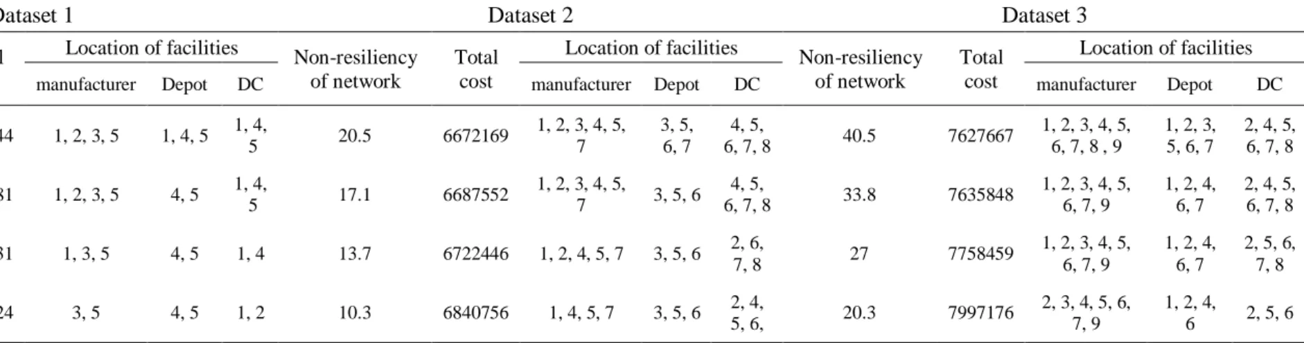
Table 2 shows the supply chain configuration changes under different values of the first and second objective function for the three datasets. As it can be seen form table 2, by increasing the resiliency of the network, the supply chain tries to reduce the criteria of node criticality, flow complexity, and node complexity through establishing less facilities and shipping links and creating a balance in the volume of input and output flows to the activated nodes, which lead to an increase in the total cost of the supply chain. The effect of the non-resiliency of the network on the cost and configuration of the supply chain is more pronounced for the larger datasets.
5-1- Conflict between cost and non-resiliency of the network
Here, the effect of changing
on the total cost of the supply chain is analyzed. Such an analysis enables a decision maker to understand the conflict between the total cost of the supply chain and the non-resiliency of the network. Note that
shows the maximum non-resiliency of the network. Figure 2 illustrates the conflict between total cost and the non-resiliency of the network for the three datasets. A first observation indicates that the cost of the supply chain increases for all datasets as non-resiliency of the network decreases. This finding could be expected because the improvement of network resiliency level does not come free. The interesting point is the pattern of cost change for different datasets under different ranges of
. In all instances, an increase in the value of
leads to a relatively linear decrease in the total cost of the supply chain, but the line steepness is different for each dataset and different ranges of
values. In other words, the relationship between cost and non-resiliency of the network is dependent on supply chain size and the range of changes in
. It is notable that the network size is represented by various datasets in which the dataset 3 is related to the largest network.205
Table 2. The optimal number of facilities under different values of objective functions
Dataset 3 Dataset 2
Dataset 1
Location of facilities Total
cost Non-resiliency
of network Location of facilities
Total cost Non-resiliency
of network Location of facilities
Total cost Non-resiliency
of network manufacturer Depot DC manufacturer Depot DC manufacturer Depot DC
2, 4, 5, 6, 7, 8 1, 2, 3,
5, 6, 7 1, 2, 3, 4, 5,
6, 7, 8 , 9 7627667
40.5 4, 5,
6, 7, 8 3, 5,
6, 7 1, 2, 3, 4, 5,
7 6672169
20.5 1, 4,
5 1, 4, 5 1, 2, 3, 5
2577144 19.5
2, 4, 5, 6, 7, 8 1, 2, 4,
6, 7 1, 2, 3, 4, 5,
6, 7, 9 7635848
33.8 4, 5,
6, 7, 8 3, 5, 6
1, 2, 3, 4, 5, 7 6687552 17.1 1, 4, 5 4, 5 1, 2, 3, 5
2678381 16.3
2, 5, 6, 7, 8 1, 2, 4,
6, 7 1, 2, 3, 4, 5,
6, 7, 9 7758459
27 2, 6,
7, 8 3, 5, 6 1, 2, 4, 5, 7
6722446 13.7
1, 4 4, 5 1, 3, 5
2682331 13
2, 5, 6 1, 2, 4,
6 2, 3, 4, 5, 6,
7, 9 7997176
20.3 2, 4,
5, 6, 3, 5, 6 1, 4, 5, 7
6840756 10.3 1, 2 4, 5 3, 5 2884224 9.8
c. Dataset 3 b. Dataset 2
a. Dataset 1
Fig 2. Conflict between cost and non-resiliency of the network for datasets 1-3
2.50E+06 2.65E+06 2.80E+06 2.95E+06 3.10E+06 3.25E+06
2 4 6 8 10 12 14 16 18 20
C
o
st
Non-resiliency of network
6.6E+06 6.7E+06 6.8E+06 6.9E+06 7.0E+06 7.1E+06 7.2E+06 7.3E+06
3 6 9 12 15 18 21
C
o
st
Non-resiliency of network
7.5E+06 7.6E+06 7.7E+06 7.8E+06 7.9E+06 8.0E+06 8.1E+06 8.2E+06 8.3E+06 8.4E+06 8.5E+06
6 13 20 27 34 41
C
o
st
196
5-2- Sensitivity analysis on the capacity of facilities
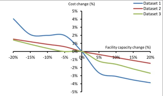
A sensitivity analysis is now completed to investigate whether the capacity adjustment of facilities, including manufacturers, warehouses, and distribution centers, can be utilized as a strategy to improve service level and supply chain cost. Figure 3 represents the changes in the supply chain cost over a range of facility capacity levels. An overall observation is that an increase in the facility capacity results in a decrease in the cost of the supply chain. A similar pattern can be seen for the three datasets; however, the magnitude of cost savings is not proportional to the networksize. That is, the curve for the dataset 1 is steeper than the curves for the datasets 2 and 3. This capacity changes do not have a significant impact on the non-resiliency of the network
Fig 3. The effect of the facility capacity change on the total cost of the supply chain
6-Conclusion
Today, many companies are affected by natural and man-made disasters, in which the lack of proper management of these incidents can have a significant negative effect on the performance of supply chains. Therefore, the design of the supply chain network under disruption risks has become a critical issue for firms. Most of the previous studies on resilient supply chain network design have focused on introducing and using various strategies to deal with disruption risks at facilities while there is scanty literature on measurement of the network resiliency. This study presented a stochastic bi-objective multi-product model to design a resilient supply chain network under random disruptions. The objectives of the proposed model were minimizing the total cost of the supply chain, as well as, minimizing the non-resiliency of the network. In addition, multiple sourcing strategy and criteria of node criticality, node complexity, and flow complexity were used to measure resiliency of the network.
The model decisions include locating manufactures, warehouses, and distribution centers, and determining the amount of production of different products in each manufacture, the amount of product transport between the different nodes of the network, and the amount of lost sales for different products in each market. Also, the possibility of partial and complete disruption of manufactures and limited capacity for facilities were considered. The validity of the proposed model was evaluated through three datasets and the results of the model implementation on them were presented.
Numerous extensions on the presented work could be aimed for future researches. Incorporating operational decisions such as routing and scheduling decisions into our proposed model can be a future research direction. In our modelfor large sizes, considering appropriate solution approaches, including Benders decomposition and Lagrangian relaxation algorithms, is another direction for future research. Also, investigating the application of the model presented in this paper to managing actual
-5% -4% -3% -2% -1% 0% 1% 2% 3% 4% 5%
-20% -15% -10% -5% 0% 5% 10% 15% 20%
Cost change (%)
Facility capacity change (%)
Dataset 1 Dataset 2 Dataset 3
197
challenges of various supply chains such as the energy supply chain can be an important future research direction.
References
Azad, N., Saharidis, G. K., Davoudpour, H., Malekly, H. & Yektamaram, S. A. (2013). Strategies for protecting supply chain networks against facility and transportation disruptions: an improved Benders decomposition approach. Annals of Operations Research, 2.125-163, 10
Baghalian, A., Rezapour, S. & Farahani, R. Z. (2013). Robust supply chain network design with service level against disruptions and demand uncertainties: A real-life case. European Journal of Operational Research, 227, 199-215.
Bérubé, J.-F., Gendreau, M. & Potvin, J.-Y. (2009). An exact ϵ-constraint method for bi-objective combinatorial optimization problems: Application to the Traveling Salesman Problem with Profits.
European journal of operational research, 194, 39-50.
Bhamra, R., Dani, S. & Burnard, K. (2011). Resilience: the concept, a literature review and future directions. International Journal of Production Research, 49, 5375-5393.
Birge, J. R. & Louveaux, F. (2011). Introduction to stochastic programming, Springer Science & Business Media.
Cardoso, S. R., Barbosa-Póvoa, A. P., Relvas, S. & Novais, A. Q. (2015). Resilience metrics in the assessment of complex supply-chains performance operating under demand uncertainty. Omega, 56,
53-73.
Chopra, S. & Sodhi, M. S. (2004). Managing risk to avoid supply-chain breakdown. MIT Sloan management review, 46, 53.
Dixit, V., Seshadrinath, N. & Tiwari, M. (2016). Performance measures based optimization of supply chain network resilience: A NSGA-II+ Co-Kriging approach. Computers & Industrial Engineering,
93205-214,
Farahani, M., Shavandi, H. & Rahmani, D. (2017). A location-inventory model considering a strategy to mitigate disruption risk in supply chain by substitutable products. Computers & Industrial Engineering, 108, 213-224.
Garcia-Herreros, P., Wassick ,J. M. & Grossmann, I. E. (2014). Design of resilient supply chains with risk of facility disruptions. Industrial & Engineering Chemistry Research, 53, 17240-17251.
Ghavamifar, A. & Sabouhi, F. (2018). An integrated model for designing a distribution network of products under facility and transportation link disruptions. Journal of Industrial and Systems Engineering, 11, 113-126.
Giri, B. C. & Bardhan, S. (2015). Coordinating a supply chain under uncertain demand and random yield in presence of supply disruption. International Journal of Production Research, 53, 5070-5084.
198
Han, X., Chen, D., Chen, D. & Long, H. (2015). Strategy of production and ordering in closed-loop supply chain under stochastic yields and stochastic demands. International Journal of u-and e -Service, Science and Technology, 8, 77-84.
Hasani, A. & Khosrojerdi, A. (2016). Robust global supply chain network design under disruption and uncertainty considering resilience strategies: A parallel memetic algorithm for a real-life case study.
Transportation Research Part E: Logistics and Transportation Review, 87, 20-52.
Hendricks, K. B., Singhal, V. R. & Zhang, R. (2009). The effect of operational slack, diversification, and vertical relatedness on the stock market reaction to supply chain disruptions. Journal of Operations Management, 27, 233-246.
Jabbarzadeh, A., Fahimnia, B. & Sabouhi, F. (2018). Resilient and sustainable supply chain design: sustainability analysis under disruption risks. International Journal of Production Research, 56, 5945-5968.
Jabbarzadeh, A., Fahimnia, B. & Seuring, S. (2014). Dynamic supply chain network design for the supply of blood in disasters: A robust model with real world application. Transportation Research Part E: Logistics and Transportation Review, 70, 225-244.
Li, Q & .Savachkin, A. (2013). A heuristic approach to the design of fortified distribution networks.
Transportation Research Part E: Logistics and Transportation Review, 50, 138-148.
Mavrotas, G. (2009). Effective implementation of the ε-constraint method in multi-objective mathematical programming problems. Applied mathematics and computation, 213, 455-465.
Nishat Faisal, M., Banwet, D. K. & Shankar, R. (2006). Supply chain risk mitigation: modeling the enablers. Business Process Management Journal, 12, 535-552.
Nooraie, S. V. & Parast, M. M. (2016). Mitigating supply chain disruptions through the assessment of trade-offs among risks, costs and investments in capabilities. International Journal of Production Economics, 171, 8-21.
Papapostolou, C., Kondili, E. & Kaldellis, J. K. (2011). Development and implementation of an optimisation model for biofuels supply chain. Energy, 36, 6019-6026.
Peng, P., Snyder, L. V., Lim, A. & Liu, Z. (2011). Reliable logistics networks design with facility disruptions. Transportation Research Part B: Methodological, 45, 1190-1211.
Sabouhi, F., Bozorgi-Amiri, A., Moshref-Javadi, M. & Heydari, M. (2018a). An integrated routing and scheduling model for evacuation and commodity distribution in large-scale disaster relief operations: a case study .Annals of Operations Research, 1-35.
Sabouhi, F., Heydari, M. & Bozorgi-Amiri, A. (2016). Multi-objective routing and scheduling for relief distribution with split delivery in post-disaster response. Journal of Industrial and Systems Engineering, 9, 17-27.
199
Sabouhi, F., Pishvaee, M. S. & Jabalameli, M. S. (2018b). Resilient supply chain design under operational and disruption risks considering quantity discount: A case study of pharmaceutical supply chain. Computers & Industrial Engineering, 126, 657-672.
Sabouhi, F., Tavakoli, Z. S., Bozorgi-Amiri, A. & Sheu, J.-B. (2019). A robust possibilistic programming multi-objective model for locating transfer points and shelters in disaster relief.
Transportmetrica A: transport science, 15, 326-353.
Santoso, T., Ahmed ,S., Goetschalckx, M. & Shapiro, A. (2005). A stochastic programming approach for supply chain network design under uncertainty. European Journal of Operational Research, 167,
96-115.
Scheibe, K. P. & Blackhurst, J. (2018). Supply chain disruption propagation :a systemic risk and normal accident theory perspective. International Journal of Production Research, 56, 43-59.
Schütz, P. & Tomasgard, A. (2011). The impact of flexibility on operational supply chain planning.
International Journal of Production Economics, 134, 300-311.
Tang, C. S. (2006a). Perspectives in supply chain risk management. International journal of production economics, 103, 451-488.
Tang, C. S. (2006b). Robust strategies for mitigating supply chain disruptions. International Journal of Logistics :Research and Applications, 9, 33-45.
Vaez, P. (2017). A New Mathematical Model for Simultaneous Lot-sizing and Production Scheduling Problems Considering Earliness/Tardiness Penalties and Setup Costs. International Journal of Supply and Operations Management, 4, 167-179.
Vaez, P., Bijari, M. & Moslehi, G. (2018). Simultaneous scheduling and lot-sizing with earliness/tardiness penalties. International Journal of Planning and Scheduling, 2, 273-291.
Vaez, P., Sabouhi, F. & Jabalameli, M. S. (2019). Sustainability in a lot-sizing and scheduling problem with delivery time window and sequence-dependent setup cost consideration. Sustainable Cities and Society, 101718.
Yin, S., Nishi, T. & Grossmann, I. E. (2015). Optimal quantity discount coordination for supply chain optimization with one manufacturer and multiple suppliers under demand uncertainty. The International Journal of Advanced Manufacturing Technology, 76, 1173-1184.
Zahiri, B., Zhuang, J. & Mohammadi, M. (2017). Toward an integrated sustainable-resilient supply chain: A pharmaceutical case study. Transportation Research Part E: Logistics and Transportation Review, 103, 109-142.
Zokaee, S., Jabbarzadeh, A., Fahimnia, B. & Sadjadi, S. J. (2017). Robust supply chain network design: an optimization model with real world application. Annals of Operations Research, 257, 15-44.