Three phase stratified sampling with ratio method of estimation

Former Faculty Member, Department of Statistics, Utkal University, Bhubaneswar, Odisha, India

1.

I

NTRODUCTION

Sometimes a survey sampler selects a large sample of units to collect information on certain variables and then select a relatively smaller sample to collect information on main character under study. This is the problem of two phase sampling. Further phases may be added, if required and the resulting sampling is termed as multiphase sampling, when the sample for the main survey is selected in more than two phases. For example, let us consider the problem of estimating the total consumer expenditure in a particular city through a sample survey, when the available information is only a list of all households in the city. If it is decided to select a sample of households, this might involve a very large sample to get a reasonably precise estimate and hence the cost involved may be considerable and prohibitive. An alternative procedure may be thought of as selecting a preliminary moderately large sample in the first phase to collect information on characteristics such as household size, occupational status etc. and these information may be used either for stratification, or for selection or in estimation procedures. In the second phase, a sub-sample from the first phase sample or an independent sample from the population is selected to observe the main character under study.

Although two-phase sampling can theoretically be extended to three or more phases, not much theoretical work is available concerning such extensions. In this paper we treat a three-phase sampling where the first phase is used for stratification, the second phase sample to observe auxiliary variables to estimate the auxiliary population characteristics to be used in estimation and the third phase sample to observe the main character under study.

2.

N

OTATIONS

Assume that the population

U

of size

N

is divided into

L

strata. Further for the

h

th

stratum

(

h

=

1 , 2 ,

…

,

L

)

denote h

N

the number of units for the

h

th stratum

' h

n

the number of units falling into

h

th stratum

s

1h after stratifying the first phase

sample

s n

₁

( )

' with the help of stratifying variable

Z

,

=

=

∑

' ' 1 L

h h

n

n

.

'' h

n

the number of units in a subsample

s

_2h from

s

_1h

( )

n

'_h for each h in the se-cond phase to observe an auxiliary variable

x

.

''' h

n

the number of units in a subsample

s

_3hdrawn from

s

_2h

( )

n

_h'' for each h in the third phase to observe the main character

y

.

=

h h

N

W

N

,

=

'

' h h

n

w

n

=

h''_' h

h

n

g

n

, a constant proportion of units sampled from the th

h

stratum at the second phase,

0

<

g

_h ≤1.

=

'''h_'' h

h

n

t

n

, a constant proportion of unit sampled from the th

h

stratum at the third phase,

0

<

t

h ≤1.

=

=

∑

1

1

Nh

h hi

i h

Y

y

N

, the mean based on

N

h units of

y

.

=

=

∑

1

1

Nh

h hi

i h

X

x

N

, the mean based on

N

hunits of

x

.

' h

y

the sample mean based on first phase sample of size in the

h

th stratum of

y

.

'' h

y

the sample mean based on second phase sample of size

n

h'' in the th

h

stratum of

y

.

''' h

y

the sample mean based on third phase sample of size

n

h'''in the th

h

stratum of

y

.

' h

x

the sample mean based on first phase sample of size

n

h' in the th

h

stratum of

x

.

'' h

''' h

x

the sample mean based on third phase sample of size

n

h'''in the th

h

stratum of

x

.

=

'

=

' ''

=

''

' ''

,

,

h h h

h h h

h h h

Y

y

y

R

R

R

X

x

x

(

)

=

=

−

−

∑

2 2

1

1

1

h

N

yh hi h

i h

S

y

Y

N

, the mean squared error based on

N

h units of

y

.

(

)

=

=

−

−

∑

2 2

1

1

1

h

N

xh hi h

i h

S

x

X

N

, the mean squared error based on

N

h units of

x

. yxh

S

population covariance between

y

and

x

in the

h

th stratum

=

+

−

2 2 2 2

2

rh yh h xh h yxh

S

S

R S

R S

' 2 yh

s

the sample mean squared error based on first phase sample of

y

in the

h

th

stratum

' 2 xh

s

the sample mean squared error based on first phase sample of

x

in the

h

th

stratum

' 2 yxh

s

the sample covariance based on first phase sample of

y

and

x

in the

h

th stra-tum

=

+

−

' 2 ' 2 '2 '2 ' '

2

rh yh h xh h yxh

s

s

R s

R s

'' 2 yh

s

the sample mean squared error based on second phase sample of

y

in the

h

th

stratum

'' 2 xh

s

the sample mean squared error based on second phase sample of

x

in the

h

th

stratum

''2 yxh

s

the sample covariance of

y

and

x

based on second phase sample in the

h

th

stratum

ρ

h the population correlation coefficient between

x

and

y

for the th

h

stratum.

3.

D

OUBLE SAMPLING FOR STRATIFICATION

Considering double sampling for stratification

=

=

∑

1 L

st h h

h

y

w y

(3.1)

where preliminary simple random sample without replacement (SRSWOR) sample

s

1

which is a subsample of first where

n

h'' units are selected according to simple random

sample without replacement (SRSWOR) out of

n

_h' units belonging to stratum

h

in the initial sample, under the assumption that an unbiased estimate of

W

_h is

w

_h

=

n

_h'

n

',

st

y

is an unbiased estimator of

Y

and the large sample variance of

y

_stis given by

( )

=









=



−



+



−







∑

_

_

2 2

' '

1

1

1

1

1

L

h yh

st y

h h

W S

V y

S

N

g

n

n

(3.2)

Minimizing the

V

( )

y

_st subject to the cost function

=

=

'

+

∑

'' 1

1

,

L

h h h

C

c n

c n

(3.3)

where

c

₁ is the cost of observing a unit in the first phase and

c

_h is the cost of observing a second phase unit, the optimum value of variance is obtained as

( )

(

(

)

)

(

)

−

+

=

∑

∑

−

2

2 2

2 1

*

Mukhopadhya

,

y, 1998

y h yh h yh h

y st _opt

S

W S

c

W S

c

_S

V y

N

C

(3.4)

where the expected cost is

( )

=

*

=

'

+

'

∑

1 h h h

,

E C

C

c n

n

c g W

(3.5)

and _{( )}

(

)









=



₋





∑



1 2

1

2 2 yh

h opt

y h yh h

c

g

S

S

W S

c

; and hence

( )

''

=

'

( )

.

h h h opt

E n

n W g

(3.6)

Pradhan (2000) considered a ratio estimator under two phase stratified sampling scheme given by

=

=

∑

" ' " 1 L

h

Rst h h

h h

y

y

w

x

Here, a preliminary simple random sample without replacement (SRSWOR) sample

s

₁

of fixed size

n

' is selected and then classified into different strata with

n

_h' units falling in the

h

th stratum

s

_1h

(

h

=

1, 2, ,

…

L

)

with

=

=

∑

' 1

'

L

h h

n

n

. In the second phase a SRSWOR sample

s

2h of size

'' h

n

is drawn from

s

1h of size ' h

n

independently of each h to observe the main variable

y

.

y

_Rst is approximately unbiased estimator of

Y

and the large sample variance of

y

_Rst is given by

( )

=









=



−



+



−







∑





2 2

' '

1

1

1

1

1

L

h rh

Rst y

h h

W S

V y

S

N

g

n

n

(3.8)

Using the cost function

=

=

'

+

∑

'' 1

1 L

h h

h

C

c n

c n

(3.9)

the optimum value of the variance of

y

_Rst is obtained as

( )

= =



_

_





_

−

_

+















=

−

∑

∑

2

2 2

1 ₂

1 1

*

L L

y h rh h rh h

h h _y

Rst _opt

S

W S

c

W S

c

S

V

y

N

C

(3.10)

where the expected cost is

( )

=

=

*

=

'

+

'

∑

* 1

1

,

L

h h h

h

E C

C

c n

n

c g W

(3.11)

( )

(

)









=



₋





∑



1 2

* 1

2 2

h opt rh

y h rh h

c

g

S

S

W S

c

, and hence

( )

"

=

' *_{( )}

.

h opt

h h

4.

T

HE SAMPLING DESIGN

Suppose a large sample

s

1 of fixed size '

n

is drawn from a population of size

N

and is stratified on the basis of the stratifying variable

Z

. Let

n

'_h denote the number of units in

s n

₁

( )

' falling into

h

th stratum

=





=

=







∑



' '

1

1 , 2 , ,

,

L

h h

h

…

L

n

n

. A sub-sample

( )

''

2h h

s

n

is drawn from

s

₁h

( )

n

'h independently for each h and an auxiliary variable

x

is observed whose frequency distribution is unknown. Further, in the third phase a sub-sample

s

₃h

( )

n

h''' is drawn from

( )

'' 2h h

s

n

independently for each h and the character of interest

y

, that is, the study variable, is observed. In the present study, simple random without replacement samples are selected in all the three phases.

5.

P

ROPOSED RATIO ESTIMATOR IN THREE PHASE SAMPLING WITH STRATIFICATION

Define an estimator of population mean

Y

of

y

under three phase sampling set up given by

=

=

∑

''' '' ''' 1 L

h

Rst h h

h h

y

y

w

x

x

(5.1)

THEOREM 5.1.

y

Rst given by (5.1) is approximately an unbiased estimator of

Y

.

PROOF.

( )

=





=







∑



''' ''

1 2 3 '''

1 L

h

Rst h h

h h

y

E y

E E E

w

x

x

, where

E E

1

,

2, and

E

3denote

expectation operators taken with respect to the first phase, second phase and third phase samples respectively.

=









=



















∑



''' ''

1 2 3 '''

1 L

h

h h

h h

y

E E

w x E

x

=





≅







∑



'' 1 2

1

,

L

h h

h

E E

w y

since









≅





''' ''

3 ''' ''

h h

h h

y

y

E

x

x

neglecting bias of

( )

''

1/

o

n

for

large value of

n

_h'''

=

=

∑

'

=

1 1 L

h h

h

Thus,

y

Rst is approximately unbiased estimator of

Y

.

THEOREM 5.2. If a first sample is a random sub-sample of fixed size

n

', the second sample is a random stratified sample from the first with fixed

g

h

(

o

<

g

h

≤

1

)

and the third sample

is a random sample from the second with fixed

t

h

(

o

< ≤

t

h

1

)

, then

( )

= =













≅



−



+



−



+



−







∑

_

_

∑

_

_

2 ₂

2

' ' '

1 1

1

1

1

1

1

1

1

L L

h yh _{h rh}

Rst y

h h h h h

W S

_{W S}

V y

S

N

g

g

t

n

n

n

(5.2)

PROOF. Now,

V y

( )

_Rst

=

E E V

_{1 2 3}

( )

y

_Rst

+

E V E

_{1 2 3}

( )

y

_Rst

+

V E E

_{1 2 3}

( )

y

_Rst

(i)

( )

=





=

















≅





−

































=





⋅



−



































−

















≅

_

_

















−









=

∑

∑

∑

∑

''' ''

1 2 3 1 2 3 '''

2 '' 2

1 2 ''' ''

2 '' 2

1 2 '

' 2

1 '

1

2

1

1

1

1

1

1

1

1

1

1

1

1

h

Rst h h

h

h rh

h h

h rh

h h

h

h rh L

h h

h

h rh

h h

y

E E V

y

E E V

w

x

x

E E

w

s

n

n

E E

w

s

g

t

n w

w s

g

t

E

n

W S

g

t

=

∑

'

1 L

h

n

(5.3)

(ii)

( )

= = = = =





=





















≅





=





−

































−

−

























≅

_

_

=













∑

∑

∑

∑

∑

''' ''

1 2 3 1 2 3 '''

1

'' 2 ' 2

1 2 1 '' '

1 1

' 2 2

1 ' '

1 1

1

1

1

1

1

1

L h

Rst h h

h h

L L

h h h yh

h h h h

L L

h h

h yh h yh

h h

y

E V E

y

E V E

w

x

x

E V

w y

E

w

s

n

n

g

g

E

w s

W S

n

n

(5.4)

(iii)

( )

=





=











 



≅

=





=



−











∑

∑

∑

''' ''

1 2 3 1 2 3 '''

'' ' 2

1 2 1 '

1

1

1

h

Rst h h

h

L

h h h h y

h

y

V E E

y

V E E

w

x

x

V E

w y

V

w y

S

N

n

(5.5) Hence,

( )

= =













≅



−



+



−



+



−







∑

_

_

∑

_

_

2 ₂ 2 ' ' ' 1 1

1

1

1

1

1

1

1

L L

h yh _{h rh}

Rst y

h h h h h

W S

_{W S}

V y

S

N

g

g

t

n

n

n

(5.6)

THEOREM 5.3. An unbiased estimator of

V y

( )

_Rst is given by

( )

= = = =



_

₋

_







₋





=









−





+



−



−

−

























−





+



−



−









∑

∑

∑

∑

'''

' ' 2

' ' '

1 1

'

2 ' 2

'

1 1

1

1

1

1

1

1

ˆ

₁

₁

1

1

1

1

h

L L

Rst h h rh

h h h h h

n L

hj Rst

h h h j

N

N

V y

n

n s

g

g

t

Nn

n

n

N

n

y

n y

g t

n

(5.7)

PROOF. Using

Est

. .

{}

as an estimator operator, we have the estimator of

V y

( )

Rst

( ) ( )

= =









=

=



−



+



−







_

_





+



−







∑

∑

2 2 ' ' 1 2 ' 1

1

1

1

ˆ

.

.

.

1

1

1

.

1

L

h yh

Rst Rst y

h h

L

h rh

h h h

W S

Est V y

V y

Est

S

Est

N

g

n

n

W S

Est

g

t

n

(5.8)

Now,

(

)

= =

−

2

=

∑∑

2

−

2 1 1

1

h N L y hj h j

N

S

y

NY

(

)

( )

= = = =

∴

−

=

−





=

−

_

−

_

∑∑

∑∑

2 2 2

1 1

2 2

1 1

.

1

.

.

ˆ

.

h h N L y hj h j N L

hj Rst Rst

h j

Est

N

S

Est

y

N Est Y

Est

y

N

y

V y

(5.9) = = = = = = = = =





=

=













=

⋅

=

∑ ∑

∑

∑

∑

∑

∑

∑

∑∑

'''

2 2 2

'''

1 1 1 1 1

2 2

1 1 1 1

1

1

h h h

h h

n N N

L L

h h h

hj hj hj

h h j h j h h j

N N

L L

h

hj hj

h h j h j

w

w

W

E

y

y

y

N

N

n

N

y

y

N

N

N

(5.10) Hence

(

)

{

( )

}

= =





−

==



−

−









∑ ∑



'''

2 2 2

''' 1 1

ˆ

.

1

h n L h

y hj Rst Rst

h h j

w

Est

N

S

N

y

y

V y

n

(5.11) = =









−

=

−

















∑

_'2

∑

_'2

1 1

1

1

.

1

1

L L

h yh h yh

h h h h

W S

w s

Est

g

n

g

n

(5.12)

= =









−

=

−

















∑

' 2

∑

'2

1 1

1

1

1

1

.

1

1

L L

h rh h rh

h h h h h h

W S

w s

Est

g

t

n

g

t

n

(5.13)

6.

O

PTIMUM ALLOCATION

Consider the cost function

= =

=

' '

+

∑

'' ''

+

∑

''' '''

1 1

L L

h h h h

h h

C

c n

c n

c n

(6.1)

where,

'

c

_{= cost of observing a unit in the first phase}

'' h

c

= cost of observing

x

-variate on a unit in the

h

th stratum in the second phase

''' h

c

= cost of observing

y

-variate on a unit in the

h

th stratum in the third phase. Here

n

''h and

''' h

n

are random variables, hence we have

( ) ( )

''

=

'

=

( )

'

=

'

h h h h h h h

E n

E g n

g E n

n W g

(6.2)

( ) ( )

'''

=

''

=

( )

''

=

'

h h h h h h h h

E n

E t n

t E n

n W g t

(6.3)

So the expected cost is given by

( )

=

*

( )

=

' '

+

'

∑

''

+

'

∑

'''

h h h h h h h

h h

E C

C

say

c n

n

c g W

n

c g t W

_(6.4)

It is required to find

n

'

,

g

h

and

t

h so as to minimize

V y

( )

Rst for a given expected

cost.

This is same as to minimize the product

(

)

= =

= =

= =

= =





_

_

+

=

+

+





_

_

























×



+



−



+



−

























=



+

+







−





×



−



+

+





∑

∑

∑

∑

∑

∑

∑

∑

2

* ' '' '''

1 1

2 2 2

1 1

' '' '''

1 1

2 2

2 2

1 1

1

1

1

1

1

L L

y

h h h h h h h

h h

L L

y h yh h rh

h h h h h

L L

h h h h h h h

h h

L L

h yh rh

y h yh

h h h

S

C

V

c

c g W

c g t W

N

S

W S

W S

g

g

t

c

c g W

c g t W

W S

S

_W

S

W S

g

=

















∑

2

1 L

h rh

h h h

with respect to

g

h

and

g t

h h.

By applying Cauchy – Schwartz inequality, the minimum value of





+













2

*

S

y

C

V

N

oc-curs if and only if

(

)

=

=

=

−

−

∑

'' '''

'

2

2 2

2 2

1

h h h h h h h

L

h rh

h yh rh

y h yh

h h h

h

c g W

c g t W

c

W S

W S

S

S

W S

g t

g

This gives the optimum value of

g

_h

and

t

_h as

( )

(

)

( )

(

)

=







₋







=

_

_

=





₋

−















∑



1 2

' 2 2 ''

2 2 '''

'' 2 2

1

and

yh rh rh h

h opt _L h opt

yh rh h

h y h yh

h

c S

S

_S

_c

g

t

S

S

c

c

S

W S

(6.5)

Substituting the value of

n

'

,

g

h opt_{( )}

and

t

h opt_{( )} in the variance expression, the optimum

variance is obtained as

( )

(

)

−

= = =

=



_

_



=



_

₋

_

₊

₋

₊















−

∑

∑

∑

1

*

2

' 2 2 2 2 '' ''' *

1 1 1

2 Rst

opt

L L L

y h yh h yh rh h h rh h

h h h

y

V

V y

c

S

W S

W

S

S

c

W S

c

C

S

N

(6.6)

7.

N

UMERICAL ILLUSTRATION

Example - 7.1

Consider a hypothetical population given in Table 1, where population

N

=

250

units are distributed in

L

=

2

strata.

Now,

(

)

= =

=

∑

2

+

∑

2

−

2

=

2 2

1 1

52.4176

y h yh h h

h h

S

W S

W Y

Y

.

Hence,

( )

=





−





=





2

1

1

1.1008

ran y

V y

S

n

N

.

TABLE 1 Strata

h

N

2

yh

S

S

xh2

Y

h

X

h

R

h

ρ

h

1 160 25 36 30 40 0.75 0.90 2 90 9 16 18 25 0.72 0.85 As

S

rh2

=

S

2yh

+

R S

h2 xh2

−

2

R

h

ρ

h

S S

yh xh, we have

=

2 1

4.75

r

S

and

S

r2₂

=

2.6064

.

For

c

_h

= =

c

1.5

the optimum variance of

y

_st in two phase stratified sampling with cost function

=

=

'

+

∑

2 '' 1

1 h h h

C

c n

c n

is given by (1.3) i.e.,

( )

=

(

+

)

−

2

1

5.76

5.2419

0.2097.

60

st _opt

c

V y

Now

V

( )

y

st _opt

<

V

( )

y

ran , if

c

1

<

0.3962

.

For

c

h

= =

c

1.5

, the optimum variance of

y

stin two phase stratified sampling with

ratio method of estimation with the cost function

=

=

'

+

∑

2 '' 1

1 h h h

c

c n

c n

is given by (1.7) i.e.

( )

=

(

+

)

−

2

1

6.9598

2.4202

0.2097.

60

Rst _opt

c

V y

Now,

( )

_Rst

<

( )

_{st opt}

opt

V

y

V

y

if

c

₁

<

0.8581

.

Setting

c

₁

=

0.25

and

c

h

=

1.5

, we find

V

( )

y

st _opt

=

0.8897

and

( )

_Rst

=

0.3705

opt

V

y

.

For

c

''h

= =

c

₁

0.25,

c

h'''

= =

c

h

1.5

, the optimum variance of

y

Rst in three phase

strati-fied sampling with ratio method of estimation is given by (5.6) i.e.,

( )

=

(

+

)

−

2 '

5.76

4.31535

0.2097

60

Rst opt

c

V y

( )

Rst

<

( )

st _opt opt

V

y

V

y

if

c

'

<

0.4367

( )

st

<

( )

Rst _opt opt

Finally, setting

c

'

=

0.05,

c

h''

=

0.25,

c

h'''

=

1.5

, we find

( )

Rst

=

0.3136

opt

V

y

.

Hence, the relative precision of the various methods can be summarized as follows: TABLE 2

Sampling Method Method of _Estimation Relative Precision 1. Simple Random Mean per unit 100 2. Stratified random Two phase 123.7271 3. Stratified random Two phase ratio 297.1120 4. Stratified random Three phase ratio 351.0204 The optimum value of the sampling fractions for two phase stratified random sampling are given by

g

_{1( )}opt

=

0.35438

and

g

2( )opt

=

0.21263.

From the expected cost we find

n

'

=

85,

E n

( )

₁''

=

19,

E n

( )

''₂

=

12

.

The optimum value of the sampling fractions for two phase stratified random sampling with ratio method of estimation are given by

g

_{1( )opt}

=

0.12784

and

g

_{2( )opt}

=

0.09470 .

From the expected cost we find

n

'

=

142,

E n

( )

₁''

=

12,

E n

( )

''₂

=

5

.

The optimum value of the sampling fractions for three phase stratified random sam-pling with ratio method of estimation are given by

g

_{1( )opt}

=

0.34939

,

( )

=

2opt

0.19632,

g

t

_{1( )}opt

=

0.19772,

t

_{2( )}opt

=

0.26066

.

From the expected cost we find

( )

( )

( )

( )

=

=

=

=

=

' '' '' ''' '''

1 2 1 2

276,

62,

20,

12,

5

n

E n

E n

E n

E n

.

Note:

n

'is determined by the expected cost,

c c

'

,

h''

,

c W

h'''

,

h,

( ) ( ) ( ) ( )

1opt

,

2opt

,

1opt

,

2opt

g

g

t

t

and may be more than

N

in a given situation. As

=

'

276

n

is more than the finite population size

N

=

250

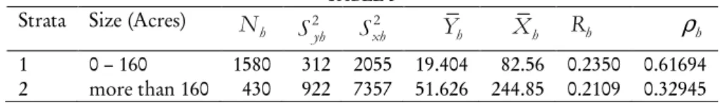
, the first phase sample size is restricted to 250, resulting in a two phase sampling design.

Example - 7.2

The following data come from a particular census in a given year, of all farms in Jefferson County, Iowa. In this example,

y

hj represents area in acres under corn and

hj

x

as total area in acres in the farm. The population is divided into two strata, the first stratum containing farms of area upto 160 acres and the second stratum containing farms of more than 160 acres.

If the cost per unit of observation is

c

=

0.5

, then for SRSWOR a sample size

n

=

100

is permissible.

TABLE 3 Strata Size (Acres)

h

N

2

yh

S

S

xh2

Y

h

X

h

R

h

ρ

h

1 0 – 160 1580 312 2055 19.404 82.56 0.2350 0.61694 2 more than 160 430 922 7357 51.626 244.85 0.2109 0.32945 Hence,

V y

( )

ran

=

5.86474

.

As

S

rh2

=

S

2yh

+

R S

h2 xh2

−

2

R

h

ρ

h

S S

yh xh, we have

=

=

2 2

1

193.3078,

2

887.3112

r r

S

S

.

For

c

_h

= =

c

0.05

, the optimum variance of

y

_st in two phase stratified sampling with the cost function

=

=

'

+

∑

2 '' 1

1 h h h

C

c n

c n

is given by (1.3) i.e.,

( )

=

(

+

)

−

2

1

13.2167

20.3806

0.30705.

50

h st _opt

c

c

V

y

Now,

V

( )

y

st _opt

<

V

( )

y

ran if

c

1

<

0.057.

For

c

_h

= =

c

0.05

, the optimum variance of

y

_st in two phase stratified sampling with ratio method of estimation with the cost function

=

=

'

+

∑

2 '' 1

1 h h h

C

c n

c n

is given by (1.7) i.e.

( )

=

(

+

)

−

2

1

16.5953

17.30164

0.30705.

50

h

Rst opt

c

c

V y

Now,

( )

_Rst

<

( )

_ran

opt

V

y

V

y

if

c

₁

<

0.103.

Setting

c

1

=

0.015,

c

h

=

0.5,

we find

V

( )

y

st _opt

=

4.8322

and

V

( )

y

Rst _opt

=

3.7637.

For

c

''h

= =

c

₁

0.015

and

= =

'''

0.5

h h

c

c

, the optimum variance of

y

_st in three phase stratified sampling with ratio method of estimation is given by (5.6) i.e.,

( )

=

(

+

)

−

2 '

13.2167

13.4373

0.30705.

50

Rst opt

c

V y

Now,

( )

_Rst

<

( )

_st

opt opt

V

y

V

y

if

c

'

<

0.03848

_and

( )

_Rst

<

( )

_Rst opt opt

V

y

V

y

if

<

'

0.0039.

c

Finally, setting

c

'

=

0.003,

c

h''

=

0.015,

c

'''h

=

0.5

, we find

( )

Rst

=

3.7037

opt

V

y

.

The optimum value of the sampling fractions for two phase stratified random sampling are given by

g

_{1( )}opt

=

0.23148,

g

_{2( )}opt

=

0.39793

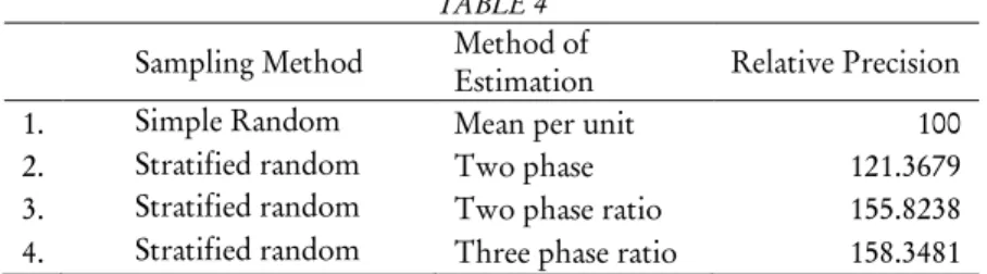
TABLE 4 Sampling Method Method of

Estimation Relative Precision 1. Simple Random Mean per unit 100 2. Stratified random Two phase 121.3679 3. Stratified random Two phase ratio 155.8238 4. Stratified random Three phase ratio 158.3481 From the expected cost we find

n

'

=

337,

E n

( )

₁''

=

61,

E n

( )

''₂

=

29

.

The optimum value of the sampling fractions for two phase stratified random sampling with ratio method of estimation are given by

g

_{1( )}opt

=

0.14511,

g

_{2( )}opt

=

0.31090.

From the expected cost we find

n

'

=

475,

E n

( )

₁''

=

54,

E n

( )

''₂

=

32

.

The optimum value of the sampling fractions for three phase stratified random sam-pling with ratio method of estimation are given by

g

_{1( )}opt

=

0.36864,

g

_{2( )}opt

=

0.19929

and

t

_{1( )opt}

=

0.22104,

t

_{2( )opt}

=

0.87600

.

From the expected cost we find

n

'

=

852,

E n

( )

₁''

=

246,

E n

( )

''2

=

36,

( )

'''

=

( )

'''

=

1

55,

2

32.

E n

E n

8.

C

ONCLUSIONS

ACKNOWLEDGEMENTS

Author is thankful to Prof. A.K.P.C. Swain for his kind suggestions. The author also wishes to express sincere gratitude to the referee for his valuable suggestions in improving the manuscript.

REFERENCES

W.G. COCHRAN (1977), Sampling Technique (Third Edition), John Wiley and Sons, New York.

A.L. FINKNER (1950), Methods of Sampling for estimating commercial peach production in North Carolina, North Carolina Agr. Exp. Stat. Tech. Bull. 91

P. MUKHOPADHYAY (1998), Theory and Methods of Survey Sampling, Prentice Hall of India, New Delhi.

J.N. PASCUAL (1961), Unbiased Ratio Estimators in Stratified Sampling, Jour. Amer. Stat. Assoc., 56, 80 – 87.

B.K. PRADHAN (2000), Some problems of Estimation in Multi-phase Sampling, Thesis submitted for the degree of Ph.D degree in Statistics of the Utkal University, Bhuba-neswar.

B.K. PRADHAN, A.K.P.C. SWAIN (2000), Two Phase Stratified Sampling with Ratio and Regression Methods of Estimations, Journal of Science and Technology, Vol. XII, Section B, 52 – 57.

J.N.K. RAO (1973), On Double Sampling for stratification and analytical surveys, Biamet-rica, 60,125 – 133.

D.S. ROBSON (1952), Multiple Sampling of Attributes, Jour. Amer. Stat. Assoc., 47, 203 – 215.

D.S. ROBSON, A.J. KING (1953), Double Sampling and the Curtis impact Surveys, Cornell Univ. Expt. Stat. Mem., 231.

SUMMARY

Three phase stratified sampling with ratio method of estimation