Essays on Asset Pricing.
Alexander Deshkovski.
A dissertation submitted to the faculty of the University of North
Carolina at Chapel Hill in partial fulfillment of the requirements for
the degree of Doctor of Philosophy in the Kenan-Flagler Business
School.
Chapel Hill
2008
Approved by
J. Conrad
M. Gultekin
R. Connolly
© 2008
Alexander Deshkovski
ALL RIGHTS RESERVED
Abstract
Alexander Deshkovski Essays on Asset Pricing
(Under the direction of J. Conrad and M. Gultekin)
I am proposing a simple theory in which an investor distinguishes between
positive and negative deviations in the portfolio value for risk estimation. The risk
of the portfolio is defined as the average futile return on the portfolio. The
investor tries to create such a portfolio that the unconditional average return is as
high as possible while conditional (negative) return on the portfolio is as small (in
absolute terms) as possible. I am not making any assumptions about the possible
distribution of the stock prices and returns. However, assuming the normal
(Gaussian) mutual distribution the solution reduces to the standard CAPM
To my mother Svetlana and my father Georii
To my wife Anjelika
Table of Contents
List of Figures ...
Chapter
I. Another Look at the Asset Allocation and Consumption Decisions ...
Introduction ...
Simple Model. Zero fraction of investor's wealth in risky asset ...
More realistic model ...
Solutions to the HJB equation ...
Monte Carlo simulation ...
Conclusion ...
II. Asset Allocation under New Definition of Risk ...
Introduction ...
Simple Models ...
Model ...
Comment about α ...
Conclusions ...
Appendices
1. Hyperbolic Absolute Risk Aversion (HARA) function ...
2. Proof of reducing the proposed theory to CAPM under
List of Figures.
Figures
1. Phase diagram of bankruptcy decisions ...
2. Simulation of volatilities ...
3. Comparison of decisions under Merton's model and my model ...
4. Comparison of Mean-Variance criterion approach
and Mean-Futile return criterion approach ...
5. Risk - Expected return preferences ...
6. Three-dimensional representation of non-Gaussian
distribution of returns on assets A and B ...
7. Contour representation of non-Gaussian distribution
of assets' A and B returns ...
8. Comparison of Mean-Variance Criterion and my model ...
9. Illustration of non-zero value of α ... 12
23
24
33
39
41
41
43
Chapter I
Another Look at the Asset Allocation
and Consumption Decisions.
1 Introduction.
Recent papers in the literature have focused on the heterogeneity of investors. Although
the heterogeneity of investors in terms of risk-aversion and discount factors may be small,
personal wealth can differ significantly. And, whereas the amount invested by any poor investor
might be small, there can be many such investors, so that their combined investment is not
small and may affect average consumption and the allocation of wealth into risky and risk-free
securities. Consequently, their behavior can affect prices in the market.
Merton’s theory [1] -[3] predicts a linear relation between wealth and decision rules.
In Merton’s world an agent’s consumption is linear in wealth and a fraction of the agent’s
wealth contributed to the risky asset is constant. However, if one relaxes some constraints,
decisions are no longer linear in wealth. This non-linearity can have grave consequences for
the notion of a representative agent. If one forms the representative agent and empirically finds
relaxation of several of these constraints has the effect that optimal decisions are no longer linear
in wealth. Consequently, in order to test the theory, one needs to integrate weighted decision
rules over wealth using the distribution of wealth values for all investors.
One of the constraints I relax is an introduction of an option to declare a bankruptcy. When
does a declaration of a bankruptcy improve the well-being of an investor? Does a possibility
of such a declaration affect the investment and consumption decisions? I find that, as with
any option, the option to declare the bankruptcy is valuable to the investor and may affect his
investment behavior. It is reasonable to expect that the value of the option is higher if the
wealth of the investor is relatively small, and the option’s value decreases with an increase in
the investor’s wealth. Because this option is not tradable, the value of the option is different
for different investors and depends upon the personal characteristics of the investor (such as
risk-aversion, discount factor, and wealth). In the present article, I argue that the effect of such
an option causes the distribution of wealth to have an effect on the consumption/investment
behavior of average investor.
One can look at this problem from a different point of view. The investor’s wealth affects
the investor’s bankruptcy option value and, therefore, the investor’s behavior. For a wealthy
investor, the value of the option to receive subsistence is less valuable compared to a poorer
investor. As a result it is difficult, and might be inappropriate, to combine investors and form
a representative agent. Indeed, consider, for example, relatively poor investors and one
wealthy investor, whose wealth is equal to the combined wealth of the poor investors. The
investor has just one option with a relatively small value (smaller than the value of any option
of an investor from the first group). As a result the wealth of small investors are much better
protected and the poor investors as a group might behave much more aggressively than the
wealthier investor. E.g. the anecdotal evidence suggests that the majority of lottery players are
poor individuals who contribute a significant fraction of their wealth to a very risky investment
(lottery); a solo investor with the same level of wealth as combined wealth of poor investors
is unlikely to contribute the same amount into a lottery. This suggests that the investment
decisions and therefore consumption decisions are not linear in wealth and the formation of
the representative agent is not warranted. Instead what one needs to do is to consider each
investor individually, find the consumption and investment rules individually and only later
aggregate (e.g. integrate with a given wealth distribution of investors). Because the rules are
not linear in wealth, the averaged decision may not necessary satisfy the optimality conditions.
As a result, it looks as if the average (or representative) investor behaves non-optimally.
1.1 Literature
One of the more important and interesting problems of finance is the portfolio selection
and consumption decisions under uncertainty. The classical approach to the problem is that of
Merton (see Merton [1] -[3] ). This approach assumes that a time-separable von
Neumann-Morgenstern utility function over the agent’s consumption represents the agent’s preferences.
increasing concave function but for the simplification of calculations in many papers the utility
function is assumed to be of a hyperbolic absolute risk aversion (HARA) family function. For
example, in Merton’s paper the utility is either or (if it reduces to
the Bernoulli utility function ). However there are other choices inside of the HARA
family for the utility function (for example, see Rubinstein [4] ). The important contribution of
the classical solution is that the consumption rate at any time is directly proportional to current
wealth, and the investment decision is simple: a fixed fraction of wealth is invested into
the risky asset and the remainder is invested in the risk-free asset. Unfortunately, that solution
also suggests that, under plausible values of the risk aversion coefficient the variance of per
capita consumption should be much larger than the observed value; this problem is known as
the equity premium puzzle (e.g. see Mehra and Prescott [6] ). There have been many attempts
to explain this puzzle. Some of these attempts question the assumption of time separability of
the utility function (e.g. [8] , [9] ); others consider models such as a habit-formation model,
while several authors look at behavioral issues.
In this paper I will present a very simple approach which allows one to explain some
intriguing problems with observed data. The most important difference between the classical
Merton model and the present paper is a change of boundary conditions. I am relaxing the
assumption that an investor experiences infinitely large negative utility if his wealth drops to
zero or below. In the real world nobody would stop consuming or die instantly as his wealth
falls below zero. In the developed economies, there are different mechanisms to prevent such
etc.). I will introduce all these mechanisms into the model by introducing a ’’safety net’’ in
the form of guaranteed consumption goods if the weighted sum of wealth and income falls to
the pre-specified value. The second difference is a consideration of a more general HARA
utility function (e.g. Rubinstein [4] ) of the form or . The third important
consideration is the income of the agent; I will consider it similar to the consideration in Merton
[2] . All three considerations contribute to the explanations described below, although for
different combinations of parameters the degree of the effect on the final result may be different.
Using this approach one can show, first, that there are plausible values of the risk aversion
coefficient such that the variance of per capita consumption is close to the observed values;
that is one can potentially explain the equity premium puzzle using this approach.
Second, the proposed solution allows for consumption/investment decisions to be
non-linear functions of wealth. As wealth decreases, the proportion of wealth consumed increases
and the investment in the risky asset also increases. Consumption is no longer independent
of the characteristics of the risky asset (such as the instantaneous rate of return or variance)
even for logarithmic utility function. The investors behave as if their risk aversion coefficient
decreases (from classical theory point of view). The simple model (in discrete time) will show
that even risk averse (rational) investors will play a lottery with negative NPV under some
conditions.
In order to understand the intuition behind the first result let’s consider the behavior of the
(in comparison to the classical Merton’s world), specifically preferring to consume more right
now (and increase utility dramatically) and later switch to the subsidized consumption goods
(hence utility does not fall to ). So, even if wealth is small, the agent will consume more
than the same agent in Merton’s world. Consequently, large oscillations in stock value will
cause relatively large oscillations in wealth, but relatively small oscillations in consumption.
Although it is not important in particular considerations, some agents will receive (constant)
subsidized consumption at some moment in time and, therefore, their volatility of consumption
is virtually zero. That effect also decreases the overall volatility of the consumption by all
investors.
On the other hand if wealth is very low and close to the value at which the agent can
switch to subsistence, he/she will find it beneficial to consume the rest of available wealth in
a short burst to boost utility, knowing that there is guaranteed utility awaiting him/her after the
wealth drops to specific level. As a result, the agent’s decision to consume depends non-linearly
on the wealth. As we will later see, consumption also depends on the financial parameters of
the risky and risk-free assets. Also, as wealth approaches the lowest possible level, the agent
may find it beneficial to risk more of his/her wealth in the hope of improving his/her situation
dramatically if there is a positive jump in price of risky asset. If the price moves down, in the
bad state, he/she does not lose a lot. So, the investor’s investment decision (and the fraction of
wealth devoted to the risky asset) is also non-linear with wealth.
I will consider an agent who has a (discounted) Bernoulli (logarithmic) utility of
to consumption rate is where and are some constants, and
is the time-preference factor (personal discount rate). can be thought of as a minimum
consumption rate the agent still can bear. If the consumption rate is below that value, the
agent dies and the utility is . is a normalization factor which is useful for showing
the invariance of the problem and for dimensional analysis.
There are two investment possibilities for the agent: either invest in a risky asset (with
fixed parameters such as instantaneous expected return and variance ) or a risk-free asset
(with constant rate of return ). In addition to the investment opportunities, the agent increases
his/her wealth by receiving income (from wages) with rate For simplicity I will assume
that the income rate is constant In this world there is also a safety net in the
form of consumption subsistence from the government if the weighted sum of wealth and
income of the agent falls to a pre-specified value . Without losing any generality
I will choose weights to be and and denote That value
represents a deterministic rate of total income at the time the agent is eligible to switch to
subsistence. If the total deterministic income is less than and the agent’s wealth is at
the agent may pay (legal, etc.) costs and forfeit his income (so, his/her total
wealth is zero and there is no income) in order to receive the consumption subsistence
starting at this time (and lasting forever). In this model I allow subsistence only in the form
of consumption goods and do not allow cash subsistence, therefore the switch to subsistence
agent is not allowed to work and receive income). The irreversible switch to consumption
subsistence is rational if where
From this inequality one can see that if the threshold is large, the consumption subsistence
must be sufficiently great to justify the switch (note that this condition is stronger than simple
for all positive and ). Intuitively, if the wealth and income of the agent is
small, the expected (integrated discounted) utility is not very large and it is beneficial for
the agent to consume everything quickly (increasing utility tremendously) and switch to the
subsistence consumption. Indeed, from Merton’s solution [1] compare the integrated utility
of where is some normalizing constant to
the integrated utility of subsistence consumption here Note that at
both integrated utilities are the same and at
the agent is better off he/she uses subsistence consumption option.
The paper is organized as follows. Section 2 deals with the very simple model which
describes an agent in the deterministic world: the agent does not participate in risky markets.
Section 3 analyzes the model under investigation and derives the Hamilton-Jacobi-Bellman
(HJB) equation. In the fourth section, I describe the solution to the HJB equation. Section 5
shows the Monte Carlo simulations to support the theoretical results and examines the problems
of interest: the equity premium puzzle and constancy/variability of the risky investment to
2 Simple Model. Zero fraction of investor’s wealth in
risky asset.
2.1 Definitions and mathematical representation.
Consider the agent with initial wealth who has income and tries to maximize the
value function
(1)
The only investment opportunity is a risk-free asset with the rate of return Also, the
agent receives steady income
The dynamics of wealth are
(2)
At the agent may choose to switch to receive consumption subsistence in the
form of consumption goods at rate (amount of consumption goods per unit of time).
2.2 Euler equation and solution to the Simple Model.
To solve the maximization problem one can express the consumption rate from eq.2
(3)
substitute it into eq.1 and solve the standard variation problem using the Euler method with
refraction boundaries. The corresponding ODE is
with boundary conditions
(5)
(6)
and refraction condition
(7)
where is the time at which the agent will choose to switch to the subsistence. If there is a
solution to eq.4 with conditions 5-7 the optimal decision will involve switching.
The solution in terms of is
(8)
where and are constants which are solutions to
(9)
(10)
(11)
The optimal consumption rate in this set-up can be found from using eq.3
(12)
In general the system 9-11 can be solved only numerically. To obtain tractable analytical
results one can consider specific values for some variables. Let , and Then
(13)
where is solution to
(15)
where
There is a real solution to eq.15 if (or ) or and
Therefore, if it is always beneficial to switch to subsistence consumption at
some moment of time; if the agent chooses to switch only if the initial wealth is smaller
than the known value
(16)
In case there is no real solution (only complex ones) to eq.15, the switch to subsistence
consumption will yield smaller integrated utility and therefore is not beneficial; in that case
and
(17)
(18)
The phase diagram below shows when the agent prefers to go bankrupt is given below on
Fig.1. Phase diagram of bankruptcy decisions. Decision rule to file or not to file
bankruptcy as a function of variables and ratio If (e.g. ) it is
always beneficial to declare the bankruptcy at some point of time. If the decision will also depend upon wealth. Is wealth is low enough (bottom right of the picture), the agent will declare the bankruptcy, if the wealth is large, the agent prefer to live on income from wages,
and income from investment, (no bankruptcy region – upper right of the picture).
People who do not participate in stock market, exhibit several interesting properties. First,
they will deliberately consume more and declare bankruptcy if A) the risk-free interest rate in
the economy is smaller then their personal discount factor or B) their initial wealth is small;
in articular if is smaller than fraction of (the specific value of the fraction depends
upon the ratio see eq.16).
The other interesting result is the consumption decision rule near the transition point. As
value . That shows us that even in the deterministic case (i.e. without allowing
the agent to participate in the stock market) one should not expect continuity of decision rules.
Although the value function is continuous at the transition point the first derivative of with
respect to is not. Consequently, that is the first order phase transition.
The important result is that under some conditions, but not always, it is beneficial to
consume more and faster and switch to subsistence rather than try to extend the life of one’s
’’independent’’ consumption. Note, that this statement might not be true if one has a negative
shock to his/her utility function as a result of transition to subsistence (e.g. if the switching
to the subsistence instantaneously decreases utility by some value). That shock can be easily
incorporated into the proposed solution but it will not contribute to the better understanding of
the problem or intuition behind it, therefore I do not consider it in the present paper.
3 More realistic model.
Although a behavior of an agent discussed in the model in previous chapter is
sub-optimal – the agent disregard risky component of the market – that behavior shows important
features that are present in the optimal behavior, namely increased (relative) consumption at
low wealth and optimality of declaration of bankruptcy. Below I consider the formal proof of
that statements. First, I will define the problem of interest and introduce variable needed to
solve the problem. Next, I will derive Hamilton-Jacobi-Bellman (HJB) equation, solve it, and
3.1 Definitions.
Consider an agent who may invest in either a risky asset with lognormal distribution of
returns or a risk-free asset with a deterministic (and constant) rate of return. I will use words
risky asset, share, stock, etc. or risk-free, bond, etc. interchangeably. I assume that there is
only one risky asset the agent can buy. He/she will contribute of his/her wealth to the
stock. The agent derives utility from a concave utility function. As an example, I will consider
the Bernoulli (logarithmic) utility of consumption where defines
the level of utility and is a normalization constant. The more general case of HARA utility
function is no harder and the choice of has no special meaning. One can
easily generalize for any Also, I assume that utility is time-separable.
The agent is rational and risk-averse. He wants to maximize his expected (discounted)
utility
(19)
where is the agent’s subjective discount factor for his/her utility, is the minimum
consumption (if the consumption falls below that the agent dies – utility is ), is the
level of utility function, and is the normalization constant.
The two investments the agent may invest in are characterized by various parameters.
The risky asset has instantaneous rate of return and volatility and the risk-free asset has
deterministic rate of return .
The dynamics of the risky asset’s price are assumed to be
where is the expected (instantaneous) rate or return and is the stock’s volatility, both of which
are assumed to be constant and and given exogenously.
The dynamics of the risk-free investment are
(21)
where we assume that the interest rate is deterministic and constant .
The agent invests a fraction of his/her wealth in the risky asset and the fraction in
the risk-free asset. In this paper, I assume that the market is frictionless and the cost of changing
the portfolio is zero. It is not difficult to introduce a flat fee for buying/selling securities; I will
investigate that case in a later paper.
The agent has income rate Therefore, the change in the agent’s wealth due to
income is If the agent becomes very poor, there is a safety net in the form of
consumption goods from the government. If the agent chooses, he/she may receive the goods
if the deterministic rate of total income falls to a pre-specified value If the total
deterministic income is less than and the agent’s wealth is at the agent may pay
(legal, etc.) costs , forfeit his/her income and receive in perpetuity the consumption
goods of value starting at this moment. As before, the switch to subsistence consumption
is assumed to be irreversible.
The decision problem of the agent is to choose decision rules for consumption and
investment rule such as to maximize value function given the initial wealth
3.2 Mathematical representation.
The agent wants to maximize his expected utility (see eq.19)
! (22)
!
where is the information available at time , subject to dynamics equations eq.s 20 and 21.
The change of the total wealth can be written as the sum of income from wages, the change
of the value of the stock, consumption, and risk-free interest
(23)
where is a fraction of total wealth contributed to the stock
One can rewrite this in the following form (suppressing the time-dependence notations
).
(24)
Substituting the dynamics of the stock from 20, and rearranging terms, one can find
(25)
where the first term represents deterministic change of wealth due to investments
income and consumption and the second term is stochastic contribution
to the wealth form the risky investment.
The multiplication table for the increments of the variables is
3.3 Constraints.
The first important constraint in my model is that consumption may not be less than
at any time Secondly, I don’t consider any liquidity constraints (such as in Longstaff [5]
), so the derivatives of may be infinite. Due to instantaneous adjustment to the desirable ratio
of investments, the state variables such as stock price and the number of holding shares
will not be present in Hamilton-Jacobi-Bellman equation.
3.4 Hamilton-Jacobi-Bellman equation.
In this subsection, I consider the infinite time horizon. This restriction is not particularly
important since it affects only the re-normalization of I will assume that the parameter is
normalized so as to take into account the probability of a death of the agent. Following Merton
[1] we may introduce the characteristic function
! (27)
where is the integrated (deterministic) utility the agent has at the time of switching to
subsistence consumption. The characteristic function may be written in similar form which
extends the integration to infinity
One can think about the equation 27 as the sum of the utilities of agent before he/she
switches to subsistence consumption (first term of the equation) and after he/she switches to
subsistence consumption (the second term). If the agent never chooses to switch to subsistence,
that can be represented by" For simplicity I will choose (although it does not
change any results and one, if so wishes, may carry out all the transformations using general
notation )
The interpretation of the value function is the total (integrated) expected utility of
the agent under optimally chosen consumption and investment decision rule given
that all available information at time is taken into account. For optimal value function
where is the integrated utility under any other decision rule or
consumption level In the text below, I suppress the function dependence notations and
will write only with the understanding that this is a function of the variable
From these considerations, we can derive that the optimal value function should satisfy
the following partial differential equation, which is known as the Hamilton-Jacobi-Bellman
(HJB) equation.
#
# (29)
where the Dynkin operator is
# #
#
# (30)
Because there is no direct dependence of on (integration of utility to infinity, see
Therefore
#
# (31)
# #
Consider time " One can find the first order conditions with respect to #
# (32)
and with respect to
# #
#
# (33)
From eq.32 and eq.33 we can easily find the optimal consumption and decision rule
(34)
and
(35)
By substituting and from eq.s 34-35 into eq.31, we obtain the differential equation for
optimal value function
# #
#
# (36)
Now we can consider time " In that case, the characteristic function is a function
of and does not depend on wealth Therefore from eq. 31 we can find that
(37)
The equation 36 has many different solutions, one of which is Merton’s solution [1] .
is described by boundary conditions. Because the eq.36 is the second order (ordinary)
non-linear differential equation it needstwo boundary conditions. The behavior of the agent near
is clearly different from the behavior of Merton’s agent; the first boundary condition is
the condition at
(38)
If the wealth of the agent is really large the influence of the safety net is insignificant and
we expect the agent to behave according to Merton’s decision rules. So the second boundary
condition is
(39)
4 Solutions to the HJB equation.
4.1 Change of variables.
The equation 36 with boundary conditions 38 and 39 can be solved using the present
notations, however, the introduction of new constants and variables helps to simplify the
solution and to show the important features of it.
Let constants be
(40)
(41)
$ (42)
Note that$ $ All units $ , and$ have the same dimensions so we
can compare them. One of the properties we will later use is
$ (44)
for all positive values of and
Introduce new variables
(45)
% (46)
(47)
& $
$ $
%
$ $ (48)
' $
$ $
%
$ $ (49)
The meaning of % is easier to understand if we look at it assuming In
this case% and% is a rate (fraction) of wealth consumption. Note that dimensions of
this new constant is also % has the same meaning but is normalized for and is a
re-normalized fraction of wealth invested into risky asset. &and'are new variables. The ODE
eq.36 is transformed into a system of relatively simple differential equations on&and' &
& & $
& ' (50)
'
' ' $
& ' (51)
It can be easily seen that if either&or'is zero they will stay zero at any and, therefore,
However the case& and' is the solution of interest. The point is a stable point
along'direction, so increasing (in other words increasing wealth) the solution converges to
– to the Merton’s solution. That is exactly what we are looking for.
So, the general solution of eq. 50-51 is
& (52)
$ '
' $
'
' (53)
where' can be found using boundary conditions eq.38 and eq.39. ' is given in implicit
form. Unfortunately there is no analytical expression for ' in explicit form. However,
general features of the solution can be easily found and are discussed below.
5 Monte Carlo simulation.
5.1 The Equity Premium Puzzle.
In that section I will show preliminary results of the possible explanation to the equity
premium puzzle which this model provides.
The following values are used for the parameters
The initial wealth was Monte Carlo step corresponds to day, there are
Monte Carlo steps.
The centered logarithms (deviations from the averages) of consumption and stock price
Fig.2. Simulation of volatilities. Volatility of logarithm of stock is much larger than the volatility of logarithm of consumption. See text for more explanations.
The volatility of the log of stock price is while the volatility of the log of
consumption is We see that the oscillation of logarithm of asset price is
much larger than the oscillation of the logarithm of the consumption. The intuition behind
the results is fairly simple. The agent knows that in the bad state he will receive subsistence
from a government in the form of consumption goods. Therefore the agent prefers to consume
more right now (and increase the utility dramatically) and, if bad state is realized, to switch
to the subsistence (and keeping the utility at bearable level). So, even if wealth is small the
5.2 The constancy of ratios.
Another example of the application of the theory is the example that the fraction of wealth
invested in the risky asset is not a constant fraction of total wealth; neither is the consumption
proportional to wealth.
Fig.3. Comparison of decisions under Merton’s model and my model. The wealth is
measured in thousands of dollars, consumption is measured in thousands of dolars per year, while is measured in non-dimentional units. The subsistance level was choosen to be
equivalent to per month.
We see that for logarithmic utility function the behavior of people may differ from linear
to level of wealth measured in tens of thousands of dollars. However, if the utility level
of switching is larger than equivalent of () $ the values of non-linearity will be
significantly larger.
The extreme values of at low wealths is the optimal behavior for poor agents. One
borrowing limits, so the poor investor will be capped at about It is sub-optimal behavior
for the agent, but the decision lies with lending authority. However, the poor people tends to
borrow (relatively) more and invest almost all their wealth into risky projects, either buying
stock, real estate, or starting risky business.
6 Conclusion.
In the present part I have considered the effect of the default possibility onto the decision
making processes, such as allocation of money into risky asset and consumption decision..
Under some conditions an investor may prefer to intensify the consumption as wealth decreases
and to declare a bankruptcy or default in order to increase the utility function.
If we assume that the investor’s wealth is very low and close to the value at which
the investor can switch to different regime (e.g. receive subsistance coupons or other
benefits), he/she will find it beneficial to consume the rest of the available wealth in a
short period of time, since the utility will increase dramatically (due to two reasons: first,
larger consumption over short period of time increases the utility function, second, there is
a guaranteed subsistence consumption, which has utility value, if the wealth drops to/below
specific level). Consequently, agent’s decision to consume depends non-linearly on the wealth.
Also, as wealth approach the lowest possible level the agent may find it beneficial to risk more
of his/her wealth in the hopes of improving his/her situation dramatically due to a positive
decisions (wealth contributed to the risky asset) are increasing with decreasing wealth and are
also non-linear with wealth.
That analysis is true not only for subsidized consumption, but also in other cases such
as strategic default (one needs just to use in 38, where is the value of utility if a firm
declares default), irreversible fire-selling to another company, etc. The analysis also holds for
different utility functions of HARA family. There are conditions then it is preferable to declare
default at low wealth.
The decisions to allocate money to risky investment and for consumption is no longer
linear in wealth, therefore a creation of the representative agent is no longer warranted. The
total money value invested by the non-linear agents in the risky market may be substantial and
it would seem that the representative agent behaves irrationally or as it has unusually high
risk-aversion coefficient; however, each single agent might behave rationally and have reasonable
Chapter II
Asset Allocation under New Definition
of Risk.
7 Introduction.
The asset pricing problem is one of the most important problems in finance. The
Markowitz and Sharpe-Lintner-Mossin theory is the classical theory of modern asset pricing
([28] -[33] ). In 1990 Markowitz and Sharpe received a Nobel Prize in Economics for the work
in Mean-Variance portfolio selection and CAPM. Many researchers and practitioners are using
CAPM in day-to-day activities. However, there is evidence in the literature that the model may
not be perfect.
One of the most important of many assumptions of CAPM is that it defines the risk of an
asset in a well diversified portfolio as its covariance with an optimal portfolio (market portfolio).
That risk stems from the non-diversifiable portion of variance. The variance includes both
positive deviations and negative deviations from the average. However, if one’s portfolio value
may increase by 50% it is hardly a risk; in contrast, if portfolio value may decrease by 50%, it
Researchers recognized long ago the limitations of the Mean-Variance Criterion and
CAPM. Although the Mean-Variance Criterion approximately holds in many cases when the
distribution of returns is not Normal (for discussion see [35] ), there have been many attempts
to improve this investment criterion. Perhaps, the simplest is the ’Geometric Mean return’
maximization. The proponents of this criterion argue that a portfolio selected based on the
maximum geometric mean return has the highest probability of achieving any given level of
wealth/return. In addition, the theory is relatively simple. The criterion assumes the utility of
potential investor in a very specific form: logarithmic. As a consequence, that theory may not
be appropriate for every investor. Also, if the returns are log-normally distributed the geometric
mean return maximization reduces to the Mean-Variance Criterion.
Another popular method is the ’Safety First’ Criterion. The first model of this type was
developed by Roy [36] . The criterion calls for minimizing the probability of the return falling
below a specified value: Prob * * For normally distributed returns the
criterion is very similar to the Mean-Variance Criterion. In the general case, it cannot be reduced
to Mean-Variance. However, the criterion does not take into account the distribution of return
below the threshold value and therefore cannot capture risk accurately. More than that, the
approach does not take into account the distribution of returns above the threshold. In other
words the criterion looks only at the ’risk’ of the portfolio disregarding possible rewards. The
second ’Safety First’ Criterion was developed by Telser [37] . His suggestion was to maximize
the return on portfolio* given that the probability of return below* does not exceed a
values and it might happen that for some combinations there are no feasible solutions/portfolios.
The second problem with the criterion is that under some conditions the best portfolio requires
unlimited borrowing. One more ’Safety First’ Criterion was introduced by Kataoka [38] : for
this criterion one maximizes the lower limit* such thatProb (* * for an
given in advance. Although the criterion takes into account the distribution of returns in the
non-desirable region, it does not consider the rewards associated with portfolio. Again, as with
first criterion, it looks only at ’the risk’ of the portfolio.
There are also criteria based on higher moments of the return distribution. They better
capture the behavior of returns and allow for a richer trade-off between reward and risk.
However, the introduction of the third moment will not capture the whole dynamics of returns
and the mathematical development of such a model is difficult.
In addition to the models mentioned above, there are models which consider semivariance
as a measure of risk. For example, one of the models maximizes the Sortino ratio [39] . The
ratio is defined as where is the expected return on portfolio, +
, - is a second lower partial moment (or semi-standard deviation), and is
a cutoff value for undesirable returns. The semi-standard deviation serves as a measure of risk
and the goal is to maximize the ratio.
A closely related set of popular models is a set of models with specific utility function
over wealth/returns. Consider, for example, the power utility function (in Rubinstein [40] it is
from Rubinstein [40] , Leland [41] derives the risk measure as ! "
! " where
is return on portfolio, while #$ is return on market portfolio.
In this paper I propose a simple single-period theory which allows one to distinguish
between positive and negative deviations in the value of a portfolio. The theory is built on
a mixture of CAPM (Sharpe’s approach and semi-variance approach) and the ’’Safety First’’
approach. The risk is defined as the average non-desirable returns on the portfolio. An investor
tries to create a portfolio so that the unconditional average return is as high as possible while
conditional non-desirable returns on the portfolio are as small (in absolute values) as possible.
I make no assumptions about the possible distribution of the stock prices. However, assuming
the normal (Gaussian) distribution it would be possible to obtain a closed form solution. It can
be shown that in the case of normal distribution the solution reduces to the CAPM solution. In
other words CAPM is a particular case of the proposed solution when the distribution of returns
is normal. If the Normal distribution is not assumed the result is stated via the integral of a
distribution density. The preliminary empirical findings agree with the observed market returns.
In addition the model allows one to explain the non-zero of the stock-market distribution and
allows for many risk factors (such as risk-free rate, inflation rate, PE ratio, book-to-market
8 Simple Models.
8.1 Linear and non-linear Models.
The CAPM and APT are linear-risk models, e.g. if one doubles the holdings in the risky
component of portfolio by borrowing at risk free rate, the risk will double. Let us consider
model with a non-linear change in risk.
The simplest possible non-linear model is to measure the risk as the probability of return
dropping below a pre-specified value. Consider, for example, an investor who is concerned
with her portfoliovalue decrease, e.g. she consider as the risk only a situation when the value
of the portfolio drops below the initial value. Assume the portfolio has expected return and
standard deviation The probability of a return below zero (decrease in value) is very
small, about Now, assume there is a risk free asset with risk-free rate of return
The investor borrows at the risk free rate the same amount as she previously invested and invests
everything into the risky asset. The probability of loss in value increases dramatically:
more than times. If the investor borrows three times the initial amount, the probability will
jump more than 100 times, to about The increase in risk is definitely not linear with the
holdings in risky component of the investor’s portfolio.
Because investors do not consider the large positive return as risky, but do consider
negative and low returns as undesirable or risky, one might be interested in developing a risk
probability of bad returns is not a good measure for several reasons. However, one can consider
the expected value of bad returns as a measure of portfolio’s risk.
8.2 ’’Uniform’’ model comparison.
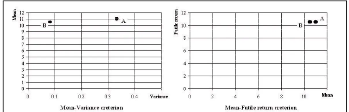
Consider two assets A and B. Asset A has a return that is uniformly distributed between
10% and 12%, while the return on asset B is uniformly distributed between 10% and 11%.
Asset A has four times the variance of asset B (and therefore higher risk) and 0.5% higher
expected return. According to the Mean-Variance criterion, a less risk-averse investor would
prefer asset A, while a more risk-averse investor would prefer asset B. There is little suggestion
from the model that the market may not be at equilibrium. However, one can see that asset
A definitely dominates asset B (in the first order stochastic dominance sense). That is, the
cumulative distribution function, ./% of asset B is always larger than ./& of asset A,
although it does not reaches 1 while ./&is zero (therefore one cannot arbitrage).
It is known that the Mean-Variance Criterion works only in the case of either quadratic
utility function (which is not a case in the real world), or when the distribution of returns
is normal (see, e.g. [34] ). However, empirically there is evidence that the returns are not
distributed normally or log-normally. Therefore there is a need for other Criteria which define
risk differently. One can consider criteria which, instead of measuring risk by variance, take
into account the undesirable results, where an investor considers the outcome as undesirable
expected value of undesirable results for the asset (or portfolio) and the unconstrained expected
value of the asset. Based on these two numbers the investor will make a decision.
Consider the same assets A and B. No matter what the investor’s value of is,
the undesirable expected return is the same for both assets, , while the
unconstrained expected return for asset A, is higher than for asset B, . Therefore
any investor with any utility function (which increases with expected return) will prefer asset
A.
Fig. 4. Comparison of Mean-Variance criterion approach and Mean-Futile return criterion approach.Using the MV approach it is impossible to tell wich asset is more preferable for investors with different utility finctions, however, the second approach shows
clearly that asset A is better for anyinvestor.
9 Model.
Different investors think about risk differently. It may be ’’Investment products offered
through XYZ are not guaranteed by XYZ, are not FDIC-insured, and may lose value’’, the
risk as simple variance of returns. Majority of less educated investors do not even understand
the notion of variance and, therefore, look for something different as a measure of downside
effects (risk).
In the model below, as a measure of risk I propose to use the expected value of ’’futile’’
returns (for formal definition see below). In order to decide whether return is not good, one can
use different benchmarks, such as (no loss in value), (to make at least what one can make
without a risk), or a market index, such as commonly used S&P 500 (beat/not beat the market).
An investor wants to maximize the unconstrained expected return of her portfolio, !
consisting of a risk-free security with risk-free return rate and weight0and risky asset
with return $' and weight 0
! 0 $' 0 - $' $' (54)
while keeping low returns under control, in other words striking the balance between
unconstrained returns and expected futile returns 1 1
( ( )
0 $' 0 - $' $' (55)
(where sub-index signifies the number of risky securities).
For a portfolio consisting of two or more risky assets the definition of expected futile
returns is very similar:
1
)
0* * 0 0 0 - * *
(56)
The most general form for that type of risk function can be written as
# + *
)
-)
- 4
)
- (57)
where & ' is the distaste function of return falling to&below acceptable threshold' and 4 & is the weight function which shows how investor weight the probability of falling short
in returns in the risk function. The & ' function can be any non-negative function for & '. Note, that & ' ' & will give the semi-variance as a measure for risk; & ' & ! & with' generates the variance of the portfolio. Other functions
such as & ' ' & ' , - or & ' ' & ' , - etc. may be
considered. & & , - places progressively smaller weight on extremely bad returns,
while & & , - almost disregards the small deviation (much less than 5 from
acceptable returns. 4 & means the investor is interested in the conditional (normalized)
expected return of undesirable states, while4 & &means that the investor fully adjusts for
the probability that the return will drop below threshold value Although only empirical data
can tell us the functions & ' and4 & I will assume the following forms: & ' ' &
and consider two possibilities for 4 & either 4 & or 4 & & The chosen form & ' ' &is linear in returns falling short by' &units, so it is placing much smaller
weight on large bad deviations from the threshold compared to semi-standard deviation case,
e.g. & ' ' & This corresponds to the investor having less risk-averse utility function.
Therefore for a portfolio of several assets one may write the following risk measures:
)
-)
- (58)
or based on absolute expected futile returns
)
- (59)
where sub-index signifies normalized returns (e.g. 4 & ), and sub-index signifies
non-normalized (e.g. 4 & &). Theoretically it is not possible to say what measure investors
are using in real life and future studies are necessary in order to distinguish between the two.
The decision can be made only by comparing them using empirical data.
9.1 Expected Futile Return Models.
The model assumes that the investors think about risk/loss only as the non-normalized
expected value of futile returns. The investor estimates the expected value of possible low
returns as they contribute to the total unconditional expected return. In other words the investor
calculates the conditional expected value of possible low returns and multiplies it by the
probability of the low return occurrence. The positive side of that definition is that the risk/loss
function, defined by futile returns, is weighted according to the probability. If the expected
futile return is very small (large negative) but the probability of it is very low, the investor will
not be worried about that greatly.
9.1.1 Optimization.
One Deterministic Asset and One Stochastic Asset. Consider the portfolio which consists
to the deterministic asset and 0to the stochastic asset. The return on that portfolio, is
0 0 * (60)
where is return on the deterministic asset and *is return on the other asset.
One can easily find the unconditional expected return on the portfolio
! 0 0 * (61)
where *is unconditional expected return on risky portfolio. The risk is determined by the low
returns of the portfolio. Investors don’t like returns below some value and consider all return
below that value as non-acceptable. Investors want to minimize risk, defined by
( ( )
0 $' 0 - $' $'
0
( ( )
- $' $'
0
( ( )
$' - $' $' (62)
That is the simplest form for risk until we specify the return distribution of risky asset. Because
later we will be interested in the risk of portfolio consisting of the Market and a risk-free asset,
I will consider the risk associated with that portfolio. Since the market portfolio consists of
many different assets, it is reasonable to assume that the distribution of return on the market
is very close to a Gaussian distribution. In the paper I will assume that the market return
distribution is indeed Gaussian # # , while the distribution of returns on any risky asset
risk-free asset and the Market, is
() # 0 #
! 0
6 # 0
6 # 6 ! (63)
and for0
(. # 0 #
! 0
6 # 0
6 # 6 ! (64)
where # ( ( # 0 ! # (65) ! ! # # (66)
and ! & is the error function ! & /
,
From equation 66 we see the
meaning of It is the leveraged Sharpe ratio The leverage coefficient is the ratio of
! or how well the portfolio is expected to perform above the minimum acceptable
level to the ! how well the portfolio is expected to perform relative to the
risk-free asset
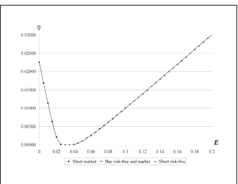
For the typical behavior of risk function as a function of expected return
Fig. 5. Risk - Expected return preferences. Vertical axis is risk function and horizontal axis is expected return ! *
As in CAPM we see that there is no reason to short the market, because in that case an
investor will have much smaller return at the same level of risk/expected loss. Also, similar
to CAPM, if the expected return on the portfolio increases, asymptotically the risk function
increases linearly with the expected return
!
#
#
6
!
#
#
Two Stochastic Assets. Now we will turn our attention to the case of two stochastic assets. The
Mean-Variance Criterion considers only the first and second moments of the distribution. That
information is sufficient if the distribution is jointly-normal (or the investors utility function is
quadratic), which is not observed in real world. That is why I will consider the joint distribution
- * which is not Gaussian. The investor looks for a trade-off between higher unconstrained
expected return
! 0 * 0 (68)
and lower expected futile return
( ( )
0 * 0 - * * (69)
Unless one know the analytical formula for the distribution function, eq. 69 cannot be
simplified.
Now we would like to compare the decisions of choosing the optimal portfolio based on
the Mean-Variance Criterion and the proposed criterion. I assume there is one risk-free asset
and only two risky assets to choose from. The return on the risk-free asset is " The
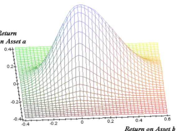
actual joint distribution of probabilities for two risky assets is a non-symmetric distribution
Fig. 6. Three-dimensional representation of non-Gaussian distribution of returns on assets A and B.
Fig. 7. Contour representation of non-Gaussian distribution of assets’ A and B returns.
The first picture gives the three dimensional view of the distribution function, while the
second gives the contours of equal values in pdf. An investor who bases her decisions on
Mean-Variance approach needs to know first and second moments of that distribution. It is very
moments. Now she can use a standard technique to find the dependence of risk, as measured
by the standard deviation of portfolio, on the expected return of portfolio. Taking into account
that she can borrow/lend at risk-free rate " she decides to contribute0 or
of her risky holdings into asset 2 and 0 " or " of her risky holdings into
asset3 She barely decreases her risk (by ) as compared to risk of asset2 and more than
twice reduces her risk as compared to asset 3 however, she increases her expected return by
roughly compared to asset2 What proportion of her wealth she puts in risk-free asset and
what proportion into the risky asset cannot be found without further assumptions about utility
function over benefits (expected return) and risks (standard deviation) of the portfolio.
The second investor, who bases his decision on the proposed model, takes into account all
points of the distribution, therefore accounting for all moments. Unfortunately, he pays the price
for that. If the distribution is not known analytically, the only way to calculate the needed values
is to calculate them numerically, which is generally resource- and time-consuming. Using eq.s
68 and 69 the investor can calculate expected return and corresponding risk for portfolios with
different composition of assets2and3 Combined with ability to borrow/lend at risk-free rate,
the investor finds the optimal portfolio to consist of0 or of asset2and 0 "#
or"# of asset3 The investor decreases his risk by as compared to risk of asset2 and
more than three times reduces the risk as compared to asset3 The increase in expected return
is approximately compared to asset2
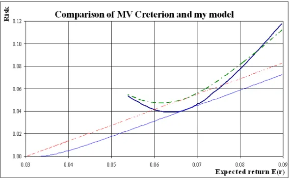
The picture below plots both decision making graphs on the same picture. One can see
Fig. 8. Comparison of Mean-Variance Criterion and my model.Dashed lines – 2-stock Efficient frontier (Capital Market line) and preference function for investor who behaves according to Mean-Variance Creterion; solid lines for investor who behaves accoring to my
model. Investor who behaves according to my model realizes higher expected return and percieves lower risk.
Although the risks are not directly comparable, the second investor will feel better, as his
risk is reduced more in relative terms. In addition he will enjoy a higher expected rate of return.
9.1.2 Partial Equilibrium in the Model.
Expected Return on Stochastic Asset. In equilibrium, all rational homogenous investors
hold the same portfolio. Everybody holds the same optimal proportion of all stochastic market
If one adds the newly issued stock to his portfolio in zero weight, the portfolio’s return still
be the same, market return, and the expected probable loss (expected value of futile returns) will
not change either. Therefore on the plane vs.! the line of new asset–market different
combinations should go through the market point, (!#* $ , #* $ The new holding should
not create room for improving both expected return and expected probable loss. Otherwise
the asset will be highly desirable and every investor starts buying it, bidding the price up and
the return down until the market finds a new equilibrium and the proportion of the new asset in
everybody’s portfolio is close to zero. Mathematically it can be expressed as that the derivatives
0
01 of portfolio consisting of the market and new asset portfolio and the portfolio consisting of
the market and deterministic asset must be the same at the point where portfolios consist of
market only. Indeed, assume that that is not the case. Consider that the derivative of the market
and new asset portfolio is less than derivative of the market and deterministic asset portfolio.
Because marginally the first portfolio provide smaller increase in the probable expected loss,
one can short (buy) the new asset (if * #( * #)), buy the market portfolio and invest
to (borrow from) the deterministic asset. The created portfolio will either have higher expected
return (at the same level of expected probable loss), or lower expected probable loss (at the
same level of expected return), or both. Therefore we conclude that
From the equation 70 and the equations 63 and 69 on risk functions we can derive the
relationship between *and other variables
*
)
* # - * # * #
# / #
#
5 # (71)
where # and - * # is the joint distribution function for the new asset’s and
market’s returns. If the joint distribution function is Gaussian, eq.71 reduces to the classical
CAPM result (see Appendix for a proof)
*
*
# # # (72)
9.2 Conditional Expected Futile Return Models.
The most important distinction of the model below is that it normalizes the expected
value of bad returns by the probability of bad return occurrence. In terms of eq. 57 the function
4 & That definition is a more accurate definition of conditional expected futile returns,
but lacks the ability to capture the weight of occurrence of the bad returns. The good side is
that the investor sees the expected bad return conditional on its occurrence. It is reasonable to
assume that the investor wants to know how much he is going to lose if something bad happens
(in some sense it is similar to Value-at-Risk). The intuition and consideration is the same as in
9.2.1 Optimality.
One Deterministic Asset and One Stochastic Asset (Market). The portfolio consists of
a deterministic asset and a stochastic asset. 0 is a fraction of total wealth contributed to the
deterministic asset and 0is contributed to the stochastic asset. The return on the portfolio,
is
0 0 # (73)
where is return on the deterministic asset and #is return on the other asset.
One can easily find unconditional expected return on the portfolio
! 0 0 # (74)
where # is unconditional expected return on risky portfolio. Again, we will introduce the
expected probable low return function, defined by
( ( )
0 # 0 - # #
( ( ) - # # 0 0 ( ( ) # - # # ( ( ) - # #
0 0 #
6 0 # ! (75)
where0 ,
#
( ( #
0 0 #
and ! & is the error function ! & /
,
Two Stochastic Assets. Consider the case of two stochastic assets. I will consider the case
where one of the stochastic assets is the asset with normally distributed unconditional returns.
The joint distribution- * # however, is not assumed to be Gaussian. The investor needs
to choose between higher unconstrained expected return
! 0 * 0 # (78)
and lower expected futile return
( ( )
0 * 0 # - * # * #
( ( )
- * # * #
(79)
As in the first model if one makes no additional assumptions about the distribution
function, that equation cannot be simplified.
9.2.2 Partial Equilibrium.
Expected Return on Stochastic Asset. In equilibrium, all rational homogeneous investors
are expected to hold the same portfolio. Therefore the proportion of each stock holdings in the
optimal portfolio is very small and can be assumed to be zero. As in first model, the derivatives
0
01 of the market and stochastic asset portfolio, and the market and deterministic asset portfolio
must be the same at point0 .
! ! (80)
From the equation 80 and the equations 78 and 79 we can derive the relationship between
2 %* %# # / # * - * *
# / # # /
# or
5 # (81)
where
%
( ( )
- * # * # (82)
%*
( ( )
* - * # * # (83)
%#
( ( )
# - * # * # (84)
#
#
(85)
# # #
(86)
and- * # is the joint distribution function for the new asset’s and market’s returns. If the
joint distribution function is Gaussian, eq.81 reduces to the classical CAPM result as in the first
model.
10 Comment about .
The proposed approach allows us to explain the existence of non-zero in regression of
asset returns on market return. Indeed, if the distribution of returns is not mutually Gaussian
line of * on # should not go through zero or, in other words, )
* # - * # * #
# / #
#
5 # (87)
where
5 )
* # - * # * #
# / #
(88)
11 Conclusions.
In this paper I have considered a model in which risk is defined differently from previous
models. Specifically the risk is defined as the expected value of the returns below a specified
threshold. The specific analytical form (e.g. functions and coefficients in eq.57) depends upon
the specific form of a representative investor’s utility function over returns. The question of
what utility function better describes the investor’s behavior is an empirical question and cannot
be solved analytically. Therefore the question what model is right (e.g. Sortino model [39] ,
Rubinstein-Leland model [40] , [41] , or model presented above) can be solved only after careful
empirical investigation.
I have defined the risk as
0
0 for the portfolio.
Based on that definition I am able to derive the partial equilibrium for the asset and have found
the expected return on the asset (eq.s 71 and 81 for two similar models). The results are simple
to interpret. The expected return on the asset is always proportional to the market premium, but
the coefficient of proportionality is no longer the (normalized) covariance of returns between
the asset and the market. More than that the coefficient may be presented as a sum of terms
each depending upon other specific risks
* $ / $ $ $ / $ $ # (89)
where $ / $ $ $ / $ $is the Taylor series of the coefficient in 71
or 81. From that equation we see that all combined risks/ $ 3 # go to zero as the
market premium goes to zero. One can orthogonalize the risks, but still all of them will depend
Several test may be designed to check the theory. The first one is to look at the equations
71 or 81 directly. One can measure distributions- * # and find, at least in principle, values
5 Knowing5it is possible to calculate the values of * # and compare it to the empirical
values.
The second approach is to check predictions for (eq.88). Knowing5one can calculate
predicted values of and compare it to the observed values.
The third one is to check eq.89.The theory predicts that the excess return on stock * #
must depend not on separate risk factors as Price/Earnings ratio 7 !, Market-to-Book ratio 8 etc., but rather on the product of these ratios to the excess market return. E.g. one should
regress * on7 ! # (or 7 ! 29 2: 7 ! # which will re-normalize
coefficient before # without changing the meaning of the equation),8 #
Size # etc. That regression should give much better results compared to regression
Appendix 1.
Hyperbolic Absolute Risk Aversion (HARA) function.
HARA family of utility functions is defined as follows.
&
& 2& 3 (90)
where2 3 and are some constants. Assuming2& 3 one can see that There are
three subfamilies of solutions.
If 2 the solution is
& 2& 3 (91)
If 2 the solution is
& 2& 3 (92)
If 2 the solution is &
3 & (93)
Appendix 2.
Proof of reducing the proposed theory to CAPM under the assumption of the mutually normal distribution of returns.
Let the mutual distribution of a stock and market returns be Gaussian
- * #
6 * # * #
* # * * * * * # # * # # # # (94)
Then, if the holdings of particular asset is very low, e.g. 0
( )
* # - * # * # * #
! # # * # *
6 #
(95)
Substituting it into 71
*
* # / #
# / #
# (96)
and solving for *one receives
* # * # * # * # (97) where * * # * # (98)
References.
[1] R.C.Merton,(August 1969), Lifetime Portfolio Selection under Uncertainty: The Continuous-Time Case,Review of Economics and Statistics,51, pp. 247-257.
[2] R.C.Merton, (1971), Optimum consumption and portfolio rules in a continuous-time model,
Journal of Economic Theory,3, pp. 373-413.
[3] R.C.Merton, (1973), An Intertemporal Capital Asset Pricing Model, Econometrica, 41, pp. 867-888.
[4] M.Rubinstein, (1975), The Strong Case for the Generalized Logarithmic Utility Model as the Premier Model of Financial Markets,The Journal of Finance,31,pp.551-571.
[5] F.A.Longstaff, (2001), Optimal Portfolio Choice and the Valuation of Illiquid Securities, The Review of Financial Studies,14, pp.407-431.
[6] R.Mehra, E.C.Prescott, (March 1985), The equity premium: A puzzle, Journal of Monetary Economics,15,pp. 145-161.
[7] R.Mehra, E.C.Prescott, (July 1988), The equity risk premium: A solution?, Journal of
Monetary Economics, 22, pp. 133-136.
[8] G.M.Constantinides, (1990), Habit Formation: A Resolution of the Equity Premium Puzzle,
Journal of Political Economy, vol.98,no.3,pp. 519-543.
[9] S.M.Sundaresan, (1989), Intertemporally Dependent Preferences and the Volatility of Consumption and Wealth,The Review of Financial Studies, vol.2,no.1, pp. 73-89.
[10] A.Deshkovski, (2004), Optimal Dynamic Trading Strategies in Markets with Information Asymmetry and Price Impact,Working paper, UNC-CH.
[11] F.Allen, D.Gale, (1992), Stock-Price Manipulation,Review of Financial Studies,5, pp.503-529.