Conditional Likelihood for Risk Estimation in
Genome Scans and Coefficient Shrinkage
by Arpita Ghosh
A dissertation submitted to the faculty of the University of North Carolina at Chapel Hill in partial fulfillment of the requirements for the degree of Doctor of Philosophy in the Department of Biostatistics, School of Public Health.
Chapel Hill 2009
Approved by:
Fred A. Wright, Advisor Fei Zou, Co-advisor
Donglin Zeng, Committee Member Andrew B. Nobel, Committee Member
c 2009 Arpita Ghosh
Abstract
ARPITA GHOSH: Conditional Likelihood for Risk Estimation in Genome Scans and Coefficient Shrinkage.
(Under the direction of Dr. Fred A. Wright and Dr. Fei Zou)
Acknowledgments
I would like to thank my advisor Dr. Fred Wright for his constant support and excellent mentorship. He has always been patient and encouraging, and I greatly value his advice on various aspects of research. I am indebted to my co-advisor Dr. Fei Zou for her guidance and insightful suggestions. She has provided me with excellent resources and advice whenever I needed it.
I would like to thank Dr. Andrew Nobel for his guidance. I have always enjoyed his availability and encouragement in addition to his expertise on the subject. I am grateful to Dr. Donglin Zeng for his assistance throughout my dissertation. This is a great opportunity to thank him for his generous support and advice. I would like to thank Dr. Kari North for her helpful comments and suggestions.
Table of Contents
Abstract iii
List of Figures viii
List of Tables ix
1 Introduction 1
2 Estimating Odds Ratios for Disease Risk in Genome Scans 6
2.1 Introduction . . . 6
2.2 Methods . . . 9
2.2.1 Significance bias (the winner’s curse) . . . 10
2.2.2 An approximate conditional likelihood . . . 11
2.2.3 The conditional MLE . . . 13
2.2.4 The mean of the normalized conditional likelihood . . . 14
2.2.5 A compromise estimator . . . 14
2.2.6 Illustrations of the conditional likelihood . . . 15
2.2.7 Conditional confidence intervals . . . 19
2.2.8 Simulations . . . 20
2.3 Results . . . 22
2.3.1 Bias . . . 23
2.3.3 Confidence coverage . . . 26
2.3.4 Sample sizes, thresholds, and covariates . . . 27
2.3.5 Analyses of published datasets . . . 28
2.4 Discussion . . . 34
2.5 Web Resources . . . 36
2.6 Supplemental Figures . . . 36
3 Analysis of Secondary Phenotypes in Case-control Studies 43 3.1 Introduction . . . 43
3.2 Methods . . . 47
3.2.1 Binary secondary phenotype . . . 53
3.2.2 Continuous secondary phenotype . . . 55
3.2.3 Simulation . . . 57
3.3 Results . . . 59
3.3.1 One binary covariate . . . 59
3.3.2 One binary and one continuous covariate . . . 63
3.4 Discussion . . . 66
4 Significance Bias for Secondary Phenotypes and GXE Interaction 70 4.1 Introduction . . . 70
4.2 Methods . . . 73
4.2.1 Significance bias . . . 75
4.2.2 An approximate conditional likelihood . . . 77
4.2.3 The conditional MLE . . . 77
4.2.4 The mean of the normalized conditional likelihood . . . 79
4.2.5 A compromise estimator . . . 80
4.2.7 Gene-environment interaction . . . 83
4.3 Results . . . 84
4.3.1 Secondary phenotype . . . 84
4.3.2 Gene-environment interaction . . . 88
4.4 Discussion . . . 90
5 Variable Selection via a Conditional Likelihood-based Penalty 93 5.1 Introduction . . . 93
5.2 Methods . . . 107
5.2.1 High-dimensional setup . . . 112
5.2.2 Numerical examples . . . 115
5.3 Results . . . 117
5.4 Discussion . . . 121
Appendix A 124
Appendix B 125
List of Figures
2.1 Behavior of the unconditional and conditional likelihoods for µ . . . 17 2.2 Estimators and confidence intervals for µwith significance thresholdc= 5 18 2.3 Means and MSEs for the three genetic models under MAF=0.25 . . . . 24 2.4 MSEs of the estimators for MAF values ranging from 0.05 to 0.5 . . . . 25 2.5 Estimates of CI coverage probability for three genetic models, MAF=0.25 26 2.6 Expectations and MSEs for three models with different MAF values . . 38 2.7 Estimates of CI coverage probability for models with different MAFs . 40 2.8 Expectations and MSEs for additive model plotted against sample size 41 2.9 Properties of the corrected estimators extended to additional settings . 42
3.1 Means and MSEs for binary secondary phenotype with one covariate . 61 3.2 Means and MSEs for continuous secondary phenotype with one covariate 63 3.3 Means and MSEs for binary secondary phenotype with covariates . . . 65 3.4 Means and MSEs for continuous secondary phenotype with covariates . 66
4.1 Expectations of estimators for β1 and β2 plotted against β1 . . . 86
4.2 MSEs of estimators for β1 and β2 plotted against β1 . . . 87
4.3 Expectations and MSEs of estimators for βg and βge plotted against βg 89
List of Tables
2.1 Original vs. corrected odds ratio estimates for published study I . . . . 31 2.2 Original vs. corrected odds ratio estimates for published study II . . . 32 2.3 Original vs. corrected odds ratio estimates for published study III . . . 33
Chapter 1
Introduction
Over the past few years a large number of genotype-phenotype associations have been reported in the genome-wide association study (GWAS) literature. However, many of these reported associations have not been replicated (Hirschhorn et al. 2002; Lohmueller et al. 2003). Among those associations that have been replicated, the estimated genetic effect size in the replication sample has often been smaller than that observed in the original GWAS (Todd et al. 2007; Yu et al. 2007; Levy et al. 2009). We investigate one of the possible reasons behind these phenomena, namely that estimates of effect sizes are upwardly-biased simply due to the fact that the genetic variants were selected for having achieved statistical significance.
inflated estimates of effect sizes for significant SNPs. This phenomenon is commonly known as the “winner’s curse” (Lohmueller et al. 2003; Z¨ollner and Pritchard 2007) or “significance bias” (Ghosh et al. 2008). For example, in a GWAS of blood pressure and hypertension for the CHARGE Consortium reported by Levy et al. (2009), effect size estimates were reported for all thirty SNPS representing the ten most significant loci for each of the three phenotypes systolic blood pressure, diastolic blood pressure, and hypertension. Each of these estimates was higher in magnitude than the estimates in a replication study reported by the Global BPgen Consortium, representing strong empirical evidence for the significance bias phenomenon.
One implication of significance bias is that if the biased estimates are used for the design of replication studies, these replication studies are likely to be underpowered. In addition, the true standard errors of risk estimates can be greatly inflated by the selection procedure. Also, standard confidence intervals for risk estimates can have very poor coverage properties. Although significance bias has been investigated and documented in detail, very few methods have been proposed for reducing or eliminating it.
via extensive simulations for a range of genetic models, minor allele frequencies and genetic effect sizes. Finally, we have applied it to published datasets to demonstrate the relevance of our approach to modern whole genome scans.
As an extension to the problem of reducing significance bias for disease risk effect, we have considered the situation where selection of a significant SNP is performed on the basis of one trait, but we wish to perform inference on the risk effect of the significant SNP for another trait (e.g. Type II diabetes and obesity). An immediate problem arises in performing valid inference for the secondary phenotype for a (retrospective) case-control design. If the secondary phenotype is associated with the disease status that forms the basis for case-control comparison, then standard logistic or linear regression applied to the secondary trait can produce severely biased estimates of the secondary risk effects (Nagelkerke et al. 1995; Jiang et al. 2006; Lin and Zeng 2008).
While the secondary analysis for case-control association studies has been addressed by many researchers in the GWAS literature (Jiang et al. 2006; Scott and Wild 2002; Richardson et al. 2007; Scott and Wild 1991; Lee et al. 1997; Lin and Zeng 2008), we describe a novel retrospective likelihood method to analyze binary or continuous secondary phenotypes. The approach models the joint distribution of the disease and secondary phenotypes such that the marginals for each phenotype respect the conven-tional models. Specifically, we specify the joint distribution such that the marginal distribution for the disease phenotype is logistic and that for the secondary phenotype is logistic or linear for binary or continuous secondary phenotypes, respectively. The approach has considerable appeal as an alternative analysis procedure for secondary phenotypes.
interaction effects. Here bias correction is necessary if the the SNPs of interest have undergone initial significance selection for the primary phenotype, and it is of interest to perform inference for the secondary effects. We demonstrate that the significance bias problem can be substantial for the secondary effects, and is closely related to the correlation between the primary and secondary effect estimates. The problem of signif-icance bias in the estimation of secondary effects has received relatively little attention in the GWAS literature. To address this problem, we have developed an extension of our conditional likelihood approach to a multivariate setting, where multiple effect co-efficients are estimated simultaneously . For implementation of this method we require the estimates of the effect sizes, their standard errors, and an estimate of the covariance between them. For secondary phenotypes, we provide formulas to estimate the relevant covariances, and the method can be implemented very easily. We have also developed the method to handle the situation where gene effects, as well as environmental effects and gene-environment interactions are all estimated simultaneously. In addition, we have shown analytically that if we first fit a reduced model for disease risk on gene only, and follow up with a full model only if the reduced model is declared significant, then the effect size estimate for the gene-environment interaction obtained from the full model is not asymptotically biased.
Chapter 2
Estimating Odds Ratios for Disease
Risk in Genome Scans
2.1
Introduction
In genetic studies, it is widely recognized that the control of genome-wide error requires the use of stringent thresholds for significance testing. For genome-wide linkage scans, standard LOD significance thresholds in the range 3.0 to 4.0 correspond to point-wise p-values in the range 10−4–10−5, depending on the model and study design (Lander and Kruglyak 1995). For modern genome-wide association studies (GWAS), 100,000 to 1 million SNP markers may be genotyped, and control of family-wise error or false discovery rates typically requires point-wise significance thresholds in the range 10−7–
10−8 (Zondervan and Cardon 2007; Todd et al. 2007; Scott et al. 2007). The use of
Cardon 2007; Allison et al. 2002; Chanock et al. 2007; Garner 2007; G¨oring et al. 2001; Hirschhorn et al. 2002; Ioannidis et al. 2001; Lohmueller et al. 2003; Siegmund 2002; Sun and Bull 2005; Yu et al. 2007; Z¨ollner and Pritchard 2007). This phenomenon has been described as a form of “winner’s curse” by Z¨ollner and Pritchard (2007) and others, or as a form of regression to the mean (Yu et al. 2007), and has profound importance for genome scans. Although the problem has been described as primarily an issue of bias, we demonstrate below that the variance of risk estimates can also be greatly inflated by the selection procedure. Moreover, standard confidence intervals for risk estimates will have very poor coverage properties, although this issue seems to have received less attention.
Consider a genome association scan for a complex disease in which 10 genomic regions contain disease genes, and each region has a 20% chance of meeting genome-wide significance. Assuming independence of regions, the genome scan has respectable power 1−(1−0.2)10 = 0.89 to achieve significance in at least one region. However,
a repeated genome scan of equal size will have power of only 0.2 for any one region, and thus likely not result in “replication” of the first study. A follow-up study might focus on a single significant region, using fewer markers and paying a lower penalty for multiple comparisons. But if the results of the initial genome scan are used as a guide, the follow-up study is likely to be underpowered, relying on an inflated estimate of locus disease risk.
who clarified that the bias can be understood largely through the behavior of Wald statistics for log odds ratios.
Although the bias is simple to understand and to document, reducing or eliminat-ing it may be nontrivial. Z¨ollner and Pritchard (2007), have described a likelihood approach which requires maximization over numerous parameters, including genotype frequencies and penetrance parameters, while conditioning on declared statistical sig-nificance. Their procedure reduces the bias in risk estimation, but cannot be performed using standard statistical software. Yu et al. (2007) have recently applied bootstrapping to correct for significance bias Both of these bias correction approaches are technically feasible for genome scans, but would be highly computationally intensive in that setting. We describe our alternative approach for estimating genetic effects in terms of odds ratios, which have numerous advantages that have made them standard for analysis of control designs (Aschengrau and Seage 2003). A crucial advantage for case-control studies is that the odds ratio (OR) may be estimated consistently, whether the study design is prospective or retrospective (McCullagh and Nelder 1989), and the OR has an interpretation distinct from nuisance parameters such as genotype frequencies. Moreover, in logistic models the OR retains interpretability in the presence of covariates, which is increasingly important for complex disease investigations.
We illustrate the performance of our approach via extensive simulations of a disease SNP analyzed by logistic regression. The simulations cover a range of models, disease allele frequencies, and OR values. Compared to nave OR estimation, our approach pro-vides greatly reduced bias and mean-squared error, particularly for the modest effect sizes likely to be encountered in complex diseases. In addition, our confidence inter-val procedure provides coverage that is accurate or slightly conservative. Performing simulations for OR values near the null presents a challenge, because significant results are very rare when applying genome-wide thresholds. We thus employ a screening ap-proach in which a deterministic trend statistic is used to identify datasets potentially significant in logistic regression.
2.2
Methods
We assume a genetic model with one parameter for the effect of disease genotype, which includes recessive, dominant, and additive models. We use β = log(OR) to denote the true loge odds ratio for disease risk conferred by a referent genotype, or for the contribution of each allele in an additive model. A single locus test statistic for disease association can be expressed as an estimate forβ divided by an estimate for its standard error,
z = ˆ β ˆ
SE( ˆβ) (2.1)
which is compared to the asymptotic null distribution N(0,1). We will refer to ˆβ and ˆ
SE( ˆβ) as na¨ıve estimators, as they are obtained from standard statistical procedures
Our approach offers marked improvements over ˆβ and standard confidence intervals. Our exposition includes mathematical and motivational details that we believe will considerably demystify the problem, which has until now appeared more obscure and complex than necessary. The performance of our new estimators is described in the Simulations subsection 2.2.8.
2.2.1
Significance bias (the winner’s curse)
When logistic regression is used to test for genetic association, the Wald statistic for genetic effect assumes the specific form of (2.1), with numerator and denominator obtained from maximum likelihood and the information matrix (McCullagh and Nelder 1989; Agresti 2007; Cox and Snell 1989). However, the essence of our approach applies to a wide variety of testing procedures, for which the key requirements typically hold: (i) asymptotic normality of ˆβ, and (ii) consistency of the standard error estimate, so that SE( ˆˆ β)/SE( ˆβ) → 1. Expressing the test statistic in the form (2.1) provides a straightforward illustration of significance bias, and points the way toward corrected estimation procedures. Related test statistics based on maximum likelihood ratios, efficient scores, or directly based on contingency tables, are all asymptotically equivalent to (2.1) for local departures from the null hypothesis H0 :β = 0 (Rao 1973), although
this asymptotic equivalence is not necessary to apply our approach. The remainder of this subsection is similar to Garner (2007), but our explicit and expanded treatment provides the grounds for later development.
For large samples, SE( ˆˆ β) does not vary markedly in repeated data realizations. Thus the estimate ˆβ and its statistical significance are highly correlated (Garner 2007) and the problem can be restated as single-parameter estimation for a truncated normal distribution. To see this, we define µ= β/SE( ˆˆ β), with Z ∼. N(µ,1). Our use of this approximation follows from the standard resultZ−µ= βˆˆ−β
SE( ˆβ)
D
sample size (Wald 1943). The statistical procedures to follow are developed entirely this “µ version” of the problem, which has been greatly simplified by the variance standardization.
Our na¨ıve estimate ofµis ˆµ=z, and the expectation can be shown analytically to be
Eµ(Z
|Z|> c) =µ+ φ(c−µ)−φ(c+µ)
Φ(−c+µ) + Φ(−c−µ), (2.2) where φ and Φ are the density and cumulative distribution function of a standard normal, respectively (see Appendix A). This is the two-sided rejection version of a result given by Garner (2007). As we detail in Results (Section 2.3), the bias can be substantial in realistic settings. In the special case of the null hypothesis µ = 0, it is clear from (2.2) that the na¨ıve estimate z is unbiased, because the two-sided testing procedure is equally likely to falsely declare positive or negative risk (i.e., a protective effect of the referent genotype). It is not clear that the lack of bias for na¨ıve estimation under the null has been fully appreciated (e.g., Figure 2 in Z¨ollner and Pritchard (2007) does not display the exact null value). However, this lack of bias requires averaging over rejections for both positive and negative z. In any significant dataset, ˆµmust be less than −c or greater than c, and so will be far from the truth under the null. In other words, the lack of bias under the null is offset by very large variance.
2.2.2
An approximate conditional likelihood
The approximating distribution ofZ suggests a correspondingly approximate likelihood for µ,
L(µ) = pµ(z) =φ(z−µ) (2.3)
variables, clinical covariates, or the effects of other SNP genotypes. It is easy to show that the maximum likelihood estimate (MLE) is ˆµ = z. A standard approach to likelihood testing for H0 : µ = 0 (Wald 1943) involves comparing the maximum
log-likelihood ratio LLR = −2ln(L(ˆµ)/L(0)) to a χ2
1 density. It is also simple to show
that here LLR =z2, so in terms of both estimation and testing, the likelihood simply
recapitulates the initial equation (2.1). The advantage to (2.3), however, is that it provides a simple and transparent approach to handle the conditioning. Acknowledging the event that the SNP is declared statistically significant, we have the conditional likelihood
Lc(µ) = pµ(z
|Z|> c) = pµ(z) Pµ(|Z|> c)
= φ(z−µ)
Φ(−c+µ) + Φ(−c−µ), (2.4)
Under (2.4), the relationship between numerator and denominator is such that, for a given z, it is quite possible that the most likely value for µ is in the interval [−c, c], even thoughz itself is conditioned to be outside that range.
2.2.3
The conditional MLE
Using the conditional likelihood, the maximum likelihood principle suggests the MLE estimator,
˜
µ1 = arg maxµLc(µ),
which can be obtained using numerical maximization for any z and c (hereafter “∼” will signify estimates based on the conditional likelihood). Note that in this setting the conditional maximum likelihood estimate provides no guarantee of unbiasedness or efficiency, a fact that does not appear to have been considered by other investiga-tors. We have already applied large-sample assumptions in constructing the conditional likelihood (2.4), but as we show below, other estimators can provide reduced bias or mean-squared error for certain ranges of µ, and therefore β.
Motivated by bias-reduction, one might attempt to directly correct the bias in ˆµby solving forµin the equationEµ(Z
|Z|> c) =z. Such an estimator has intuitive appeal,
representing the value ofµfor which, after conditioning on significance, we would have expected to observe z. Perhaps surprisingly, this “bias-correction” estimator in fact turns out to be ˜µ1. To see this, we take the derivative of the conditional likelihood with
respect toµ, for which the identity L0c( ˜µ1) = 0 implies
z = ˜µ1+
φ(c−µ˜1)−φ(c+ ˜µ1)
Φ(−c+ ˜µ1) + Φ(−c−µ˜1)
, (2.5)
Comparing equation (2.3) to (2.5) implies that the bias-correction estimator and ˜µ1 are
the same. Similar estimators have been examined in the context of sequential clinical trials, in which effect parameters are estimated only after a stopping boundary has been reached (Liu et al. 2004). Despite its secondary motivation as a bias-correction estimator, the conditional MLE ˜µ1 is not in fact unbiased, due to nonlinearity in the
special optimality properties, and other estimators may be reasonable. Nonetheless, we will show that ˜µ1 is markedly improved over the na¨ıve estimator, both in terms of bias
and mean squared error.
2.2.4
The mean of the normalized conditional likelihood
The motivation to reduce mean-squared error (MSE) suggests another, perhaps less-obvious estimator,
˜ µ2 =
R∞
−∞µLc(µ)dµ
R∞
−∞Lc(µ)dµ
, (2.6)
which is easily calculated numerically. ˜µ2 is the mean of the random variable following
the distributionLc(µ), normalized to be a proper density. ˜µ2 has favorable MSE
prop-erties when averaged across a wide range of µ. This fact follows from an interpretation of ˜µ2 as a posterior mean in a Bayesian treatment of the problem with a flat prior on
µ (Leonard and Hsu 1999). However, ˜µ2 is considered here as an entirely frequentist
estimate, with bias and error examined at each value ofµ and judged accordingly. For |z| near the boundary c, ˜µ2 typically represents a less aggressive shrinkage toward 0
compared to ˜µ1.
2.2.5
A compromise estimator
In the treatment below, we will see that the conditional likelihood is typically skewed, and so ˜µ1 and ˜µ2can differ appreciably for certain values ofz. ˜µ2 can show higher MSE
than ˜µ1 for µ near zero, but is more favorable for µ away from zero, while the bias of
˜
µ1 and ˜µ2 can be of opposite signs for µ near the significance threshold c. Thus as a
practical compromise we also examine the estimator
˜
which balances the strengths of ˜µ1 vs. ˜µ2.
2.2.6
Illustrations of the conditional likelihood
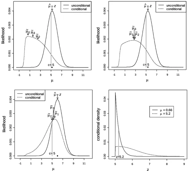
Figure 2.1 illustrates the conditional and unconditional likelihoods assuming an illus-trative constant threshold c= 5.0. Panels (a)-(c) correspond toz = 5.2, 5.33, and 6.0, respectively. For each panel, the unconditional likelihood is centered and maximized at z (indicated by a dot on each plot). For panel (a), when z is only slightly above the threshold, the conditional likelihood is in contrast shifted aggressively towards zero ( ˜µ1 = 0.66, ˜µ2 = 2.53, ˜µ3 = 1.60). When z is well above the threshold (z=6.0, panel
(c)) this shift is much smaller ( ˜µ1 = 5.48, ˜µ1 = 4.94, ˜µ1 = 5.21). For an intermediatez
(panel (b)), the shift is intermediate. Note that our estimates are obtained here for the µ version of the problem, and the conversion β = µSE( ˆˆ β) must be performed before the results are interpreted on the log-odds scale.
As desired, the conditional likelihood shows a clear shift toward zero. But why is the shift so extreme, e.g., when z = 5.2? Such a z-value (which is equivalent to ˆ
µ) has already met genome-wide multiple-testing correction for statistical significance,
but a shrinkage from ˆµ = 5.2 to ˜µ1 = 0.66 (for example) will effect a corresponding
proportional reduction in the log odds ratio. Thus it seems our proposed estimation procedures can often adjust the estimated effect size to bepractically insignificant. To see why the result is reasonable, consider that the conditional likelihood, as a frequentist construction, makes no judgment about the prior plausibility of various values of µ. When presented with a value z for each µ, it considers only the chance that z would have arisen, given that |z|> c.
for z, not likelihoods. However, for a fixed value of z, the relative heights of the two curves reflect the conditional likelihoods for the two competing values of µ. From the curves we can see the valuez = 5.2 is 2.77 times more likely to arise whenµ= 0.66 than when µ= 5.2. Expressed in another way, when µ values are truly of large magnitude, then z tends to overshoot the threshold cby a greater amount than was observed here forz = 5.2. Thus in this instance we would conclude thatµis not likely to be of large magnitude.
Our three proposed estimators can be easily computed numerically, and simpleRand Excel programs to do so are available at our website www.bios.unc.edu/~fwright/
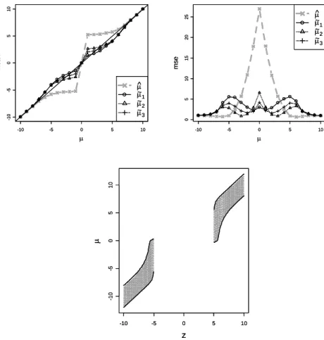
genomebias. Using the threshold c = 5 for illustration, we have calculated the
con-ditional expectations and MSEs for the three estimators, shown in Figure 2.2[(a)-(b)]. The three corrected estimators provide dramatically reduced bias compared to the na¨ıve estimator for much of the range of µ. For µ = 0, by symmetry all estimators are un-biased. For |µ| considerably larger than c, all methods will give estimators near z and will be nearly unbiased. The corrected estimators tend to under-correct for small µ and over-correct for large µ. The conditional MLE ˜µ1 can be viewed as a first-order
attempt to correct the bias, while the data z occupies the same range whether µ is small or large. In a sense, the corrected estimate splits the difference between the two extremes, leading to the observed pattern.
The MSE for ˆµ = z is extremely large for µ near zero, as predicted. MSEs for the corrected estimators are considerably smaller in the range of small to moderate µ. As described above, these estimators are easily converted to the corresponding
improved log(OR) estimators ˜β1, ˜β2, ˜β3. Moreover, for large samples the bias and MSE
μ
lik
elihood
unconditional conditional
-1 1 3 5 7 9 11
0. 000 0. 001 0. 002 0. 003 0. 00 4 c= 5
μ^=z
μ ~ 1 μ ~ 2 μ ~ 3 μ lik e lihood unconditional conditional
-1 1 3 5 7 9 11
0. 000 0. 001 0. 002 0. 003 0. 004 c= 5
μ^=z
μ ~
1 μ~2
μ ~ 3 μ lik elihood unconditional conditional
-1 1 3 5 7 9 11
0. 00 0 0. 00 1 0. 00 2 0. 00 3 0. 00 4 c= 5
μ^=z
μ ~ 1 μ ~ 2 μ ~ 3
5 6 7 8 9
0 .00 0. 0 1 0. 0 2 0. 03 0 .04 z c on dit io nal d ens it
y μ = 0.66
μ = 5.2
z=5.2 μ lik elihood unconditional conditional
-1 1 3 5 7 9 11
0. 000 0. 001 0. 002 0. 003 0. 00 4 c= 5
μ^=z
μ ~ 1 μ ~ 2 μ ~ 3 μ lik e lihood unconditional conditional
-1 1 3 5 7 9 11
c= 5
μ^=z
0. 000 0. 001 0. 002 0. 003 0. 004 μ ~
1 μ~2
μ ~ 3 μ lik elihood unconditional conditional
-1 1 3 5 7 9 11 5 6 7 8 9
0 .00 0. 0 1 0. 0 2 0. 03 0 .04 z c on dit io nal d ens it
y μ = 0.66
μ = 5.2
z=5.2 c= 5
μ^=z
0. 00 0 0. 00 1 0. 00 2 0. 00 3 0. 00 4 μ ~ 3 μ ~ 1 μ ~ 2
-10 -5 0 5 10 -1 0 -5 0 5 1 0 μ m ean μ ^ μ ~1 μ ~ 2 μ ~ 3
-10 -5 0 5 10
0 5 10 15 20 25 μ ms e μ^ μ ~ 1 μ ~ 2 μ ~ 3
-10 -5 0 5 10
-1 0 -5 0 5 1 0 z μ
-10 -5 0 5 10
-1 0 -5 0 5 1 0 μ m ean μ ^ μ ~1 μ ~ 2 μ ~ 3
-10 -5 0 5 10
0 5 10 15 20 25 μ ms e μ^ μ ~ 1 μ ~ 2 μ ~ 3
-10 -5 0 5 10
-1 0 -5 0 5 1 0 z μ
Figure 2.2: Estimators and confidence intervals for µwith significance thresh-old c= 5.
2.2.7
Conditional confidence intervals
Proper interpretation of the corrected µ estimates requires an understanding of esti-mation error, conditioned on statistical significance. Standard confidence interval (CI) procedures fail in this setting. For example, after conditioning on significance, a stan-dard 95% CI for µ cannot contain 0, for otherwise it would not have been significant. Thus, whenµ= 0 the standard CI procedure has zero conditional coverage probability. Z¨ollner and Pritchard (2007) addressed this issue by using a standard maximum like-lihood ratio approach applied to the conditional likelike-lihood. In our setting, a 1−η CI created in this manner would consist of allµvalues such that 2ln(Lc( ˜µ1)/Lc(µ))≤q1−η,
whereq1−η is the 1−ηquantile of aχ21 density. However, we have shown via numerical
integration that in the µ version of the problem, the true coverage probability of this CI procedure can exhibit markedly conservative or anticonservative departures from 1−η, depending on the true µ. Approaches using the second derivative at lnLc( ˜µ1)
to estimate the error variance also fail. The difficulty arises because the conditional m.l.e is not normally distributed, nor is the shape ofLc(µ) approximately normal for a
realized dataset.
To create confidence intervals with correct conditional coverage, we return to the original Neymanian concept of a confidence region (Rao 1973; Lehmann and Casella 1983), which can always be applied when the distribution of a test statistic is known for each value of the unknown parameter. Let A(µ,1−η) be an acceptance region depending on µsuch that
Pµ Z ∈A(µ,1−η)
|Z|> c= 1−η .
1−η for any µ. Among possible acceptance regions, we choose A(µ,1−η) as the interval between theη/2 and 1−η/2 quantiles of the conditional densitypµ(z
|Z|> c).
Note that, although we have presented three competing point estimates for µ, our procedure yields only a single CI. Figure 2.2 (c) shows the upper and lower confidence limits for our CI procedure for each z. Note that the limits are wider when |z| is near c, reflecting less certainty about µ, and can even contain µ = 0. This does not contradict the statistical significance - the intent of the procedure is to obtain correct coverage for anyµ(includingµ= 0) after conditioning on significance. The conversion of the confidence limits to the β scale is
µlowerSE( ˆˆ β), µupperSE( ˆˆ β)
. Although our procedure is guaranteed correct conditional coverage in the idealized µsetting, our CI forβrelies on large-sample normality assumptions for ˆβ. Thus we investigate empirical coverage of our procedure in the Results Section.
2.2.8
Simulations
To describe our simulations, we begin with basic notation for disease association stud-ies. We let y denote the disease status (0=control, 1=case) for an individual, and x denote the SNP genotype predictor value. For a bi-allelic SNP with major allele A and minor allele a, x is defined as follows for genetic models with respect to a:
Recessive
g =
0, AA 0, Aa 1, aa
Additive
g =
0, AA 1, Aa 2, aa
Dominant
g =
We assume the logistic model for a randomly sampled individual in the population
log (P(Y = 1|x)/(1−P(Y = 1|x))) =α+βx,
for some α, and β is the log odds ratio for a unit increase in x. Rather than speci-fying α directly, it is more interpretable to solve for α for a specified allele frequency and disease prevalence π. The marginal frequency of x is denoted p(x), and is easily calculated from Hardy-Weinberg assumptions. With fixed disease prevalence, the iden-tity π =P
x
exp(α+βx)
1+exp(α+βx)p(x) was used to calculate α. Finally, solving for the genotype
probabilities conditioned on case/control status yields
P(X =x|Y = 1) = p(x) π
exp(α+βx) 1 + exp(α+βx)
and P(X =x|Y = 0) = p(x) 1−π
1
1 + exp(α+βx) .
A standard result is that logistic modeling forβapplies even when the data are sampled retrospectively (McCullagh and Nelder 1989).
Each dataset was simulated and analyzed in R v.2.5.1. We will denote the total sample size n = ncases +ncontrols, and ncases = ncontrols throughout. Most simulations
2001), and ensures that simulations span the range from low power to high power. For simplicity, we used c = 5.0, corresponding to a single p-value of 5.7×10⁻⁷, near the genome-wide threshold considered by others (Zondervan and Cardon 2007; Todd et al. 2007; Scott et al. 2007).
For recessive models we considered MAF values of 0.25 and 0.5 - lower values cre-ated small expected cell counts that were problematic for sample sizes of 500 in each group. For the additive and dominant models we considered minor allele frequency (MAF) values of 0.05, 0.1, 0.25, and 0.5. A single setup consisted of the genetic model, MAF, and β, and sufficient simulations were performed for each setup to obtain 1000 significant datasets. Setups with β = 0 required on the order of 109−1011 simulations
for this rarefied threshold. We sped up the analysis by first applying a chi-square test (Cochran-Armitage trend test for the additive model) to the datasets, which can be obtained without iterative maximization. The chi-square statistic was determined to have a close correspondence to z2 obtained from the more computationally intensive
logistic regression, and a chi-square statistic≥24 was determined to capture essentially all datasets withz2 ≥c2 = 25. Datasets meeting the chi-square criterion were analyzed via logistic regression inR glm. For datasets achieving final significance as determined by logistic regression, ˆβ and ˆSE( ˆβ) were used to obtain ˜β1, β˜2, β˜3, and conditional
confidence intervals.
2.3
Results
2.3.1
Bias
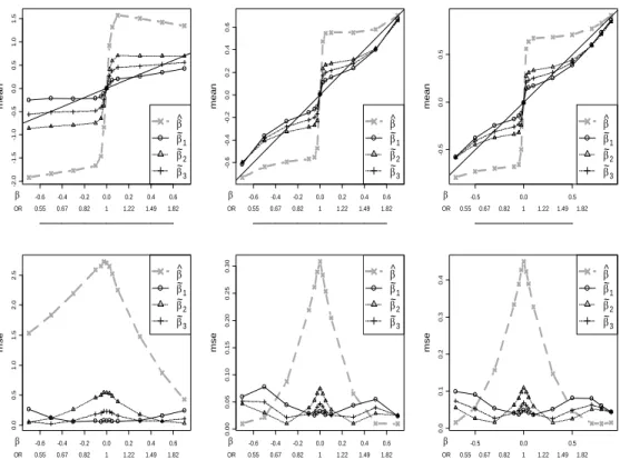
The top row of Figure 2.3 plots the means for each of the na¨ıve and corrected estima-tors vs. β (with corresponding OR values) for all models, with MAF=0.25. The na¨ıve estimator shows very large bias, especially for moderate β. All of the corrected esti-mators show dramatically reduced bias across most of the range examined. For each model, the corrected estimates tend to under-correct for small (magnitude) β while overcorrecting for large β. All of the methods become nearly unbiased for large β, as they must, for the conditional and unconditional likelihoods are nearly identical when |z| is well beyondc. In terms of bias, ˜β1 performs best among the corrected estimates
for small . However, the over-correction of the conditional MLE can be substantial for moderate to largeβ, especially for the recessive model. ˜β2 shrinks the estimates toward
zero less dramatically, resulting in under-correction for a larger part of the range ofβ. ˜
β3 strikes a balance between the other two corrected estimates, and has much improved
bias for moderate β under the recessive model. All estimators are effectively unbiased for β = 0. A subtle asymmetry in the plots for positive and negative log(OR), most evident in the recessive model, occurs because MAF<0.5 and, for a fixed prevalence, the logistic interceptα depends on β.
2.3.2
Mean squared error
-0.6 -0.4 -0.2 0.0 0.2 0.4 0.6 -2 .0 -1 .5 -1 .0 -0 .5 0 .0 0 .5 1 .0 1 .5 mea n β ^ β ~ 1 β ~ 2 β ~ 3
0.55 0.67 0.82 1 1.22 1.49 1.82
β
OR
-0.6 -0.4 -0.2 0.0 0.2 0.4 0.6
-0 .6 -0 .4 -0 .2 0 .0 0 .2 0 .4 0 .6 mea n β^ β ~ 1 β ~ 2 β ~ 3
0.55 0.67 0.82 1 1.22 1.49 1.82
β
OR
-0.5 0.0 0.5
-0 .5 0 .0 0 .5 mea n β ^ β ~ 1 β ~ 2 β ~ 3
0.55 0.67 0.82 1 1.22 1.49 1.82
β
OR
-0.6 -0.4 -0.2 0.0 0.2 0.4 0.6
0. 0 0. 5 1. 0 1. 5 2. 0 2. 5 mse β ^ β ~ 1 β ~ 2 β ~ 3
0.55 0.67 0.82 1 1.22 1.49 1.82
β
OR
-0.6 -0.4 -0.2 0.0 0.2 0.4 0.6
0. 0 0 0. 05 0 .10 0. 15 0. 2 0 0. 25 0 .30 mse β^ β ~ 1 β ~ 2 β ~ 3
0.55 0.67 0.82 1 1.22 1.49 1.82
β
OR
-0.5 0.0 0.5
0. 0 0. 1 0. 2 0 .3 0.
4 β^
β ~ 1 β ~ 2 β ~ 3
0.55 0.67 0.82 1 1.22 1.49 1.82
β
OR
mse
Figure 2.3: Expectations and mean squared errors for the three genetic mod-els under MAF=0.25.
For the three models and MAF=0.25, the corrected estimators show greatly improved performance for much of the range of β. Top row: expected values for the na¨ıve and conditional likelihood estimators vs. β. Bottom row: mean squared errors for the es-timators. The y-axes for the MSE plots are rescaled to highlight details - the MSE is considerably larger for the recessive model due to scarcity of the risk homozygotes.
the MSE( ˜β1) is fairly low, while MSE( ˜β2) peaks. For larger magnitude β, the roles
reverse. As expected, ˜β3 exhibits a more even MSE across the range, and represents
a reasonable choice for stable error characteristics. For the additive and dominant models, ˆβ exhibits very low MSE for large β. This phenomenon is not as attractive as it appears, essentially resulting from a boundary effect in which ˆβ is nearly constant because z is just barely significant. In particular, for β outside of the plotted range, m.s.e( ˆβ) rises again to the var( ˆβ ) value encountered in the unconditional setting.
-0.6 -0.4 -0.2 0.0 0.2 0.4 0.6 0. 0 0 .5 1. 0 1 .5 MAF=0.05 ms e β^ β ~ 1 β ~ 2 β ~ 3
0.55 0.67 0.82 1 1.22 1.49 1.82
β OR
-0.6 -0.4 -0.2 0.0 0.2 0.4 0.6
0. 0 0. 5 1. 0 1. 5 MAF=0.1 mse β ^ β ~ 1 β ~ 2 β ~ 3
0.55 0.67 0.82 1 1.22 1.49 1.82
β OR
-0.6 -0.4 -0.2 0.0 0.2 0.4 0.6
0. 0 0. 5 1. 0 1. 5 MAF=0.25 mse β^ β ~ 1 β ~ 2 β ~ 3
0.55 0.67 0.82 1 1.22 1.49 1.82
β OR
-0.6 -0.4 -0.2 0.0 0.2 0.4 0.6
0. 0 0. 5 1. 0 1. 5 MAF=0.5 mse β ^ β ~ 1 β ~ 2 β ~ 3
0.55 0.67 0.82 1 1.22 1.49 1.82
β OR
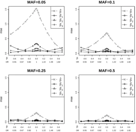
Figure 2.4: Mean squared errors of the estimators vs. β for MAF values ranging from 0.05 to 0.5.
The additive model is assumed, with n = 1000. The MSEs drop for larger MAF, but the relative performance of the estimators is maintained.
-0.6 -0.4 -0.2 0.0 0.2 0.4 0.6 0. 70 0. 75 0. 8 0 0. 85 0. 90 0 .95 1. 00 co ve ra g e
0.55 0.67 0.82 1 1.22 1.49 1.82 β
OR
-0.6 -0.4 -0.2 0.0 0.2 0.4 0.6
0. 70 0. 75 0. 8 0 0. 85 0. 90 0 .95 1. 00 co ve ra g e
0.55 0.67 0.82 1 1.22 1.49 1.82 β
OR
-0.5 0.0 0.5
0. 70 0. 75 0. 8 0 0. 85 0. 90 0 .95 1. 00 co ve ra g e
0.55 0.67 0.82 1 1.22 1.49 1.82 β
OR
RECESSIVE ADDITIVE DOMINANT
-0.6 -0.4 -0.2 0.0 0.2 0.4 0.6
0. 70 0. 75 0. 8 0 0. 85 0. 90 0 .95 1. 00 co ve ra g e
0.55 0.67 0.82 1 1.22 1.49 1.82 β
OR
-0.6 -0.4 -0.2 0.0 0.2 0.4 0.6
0. 70 0. 75 0. 8 0 0. 85 0. 90 0 .95 1. 00 co ve ra g e
0.55 0.67 0.82 1 1.22 1.49 1.82 β
OR
-0.6 -0.4 -0.2 0.0 0.2 0.4 0.6
0. 70 0. 75 0. 8 0 0. 85 0. 90 0 .95 1. 00 co ve ra g e
0.55 0.67 0.82 1 1.22 1.49 1.82 β
OR
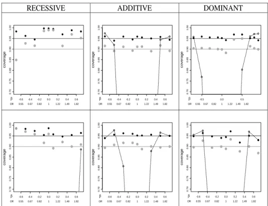
Figure 2.5: Estimates of the CI coverage probability plotted against β for the three genetic models, MAF=0.25.
Black dots correspond to 95% CIs, grey dots to 90% CIs. The dashed curves represent coverage of standard 95% CIs which do not acknowledge the significance selection. Top row: n = 1000 (500 cases and 500 controls). Bottom row: n = 2000 (1000 cases and 1000 controls). Coverage is close to nominal, except for regions of over-coverage in the recessive model due to small cell counts (note that the y-axis range begins at 0.7). For all models, the coverage will approach the nominal value as the sample size increases further.
2.3.3
Confidence coverage
improves further, with a region of modest over-coverage for recessive models. Results for other MAF values are similar, and are presented in Supplemental Figure 2.7.
2.3.4
Sample sizes, thresholds, and covariates
Our setup conditions represent a wide range of realistic scenarios, but cannot represent all situations and complicating factors. Fortunately, the large-sample behavior of the constructed approximate likelihood provides considerable robustness for our conclu-sions. Supplemental Figure 2.8 shows the results of increasing sample size for several realisticβvalues for the additive model when MAF=0.25. The bias and MSE for all the estimators are reduced as the sample size increases. For each sample size, the corrected estimators show superior bias and MSE compared to the na¨ıve estimator.
In maximum likelihood settings, the distribution of the Wald test statistic is largely driven by β/SE( ˆβ). This is also true for our conditional likelihood, because β/SE( ˆβ) determines the non-centrality of the z-statistic. For a fixed ratio ncases : ncontrols,
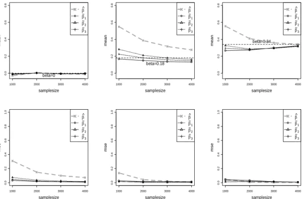
the standard error is proportional to 1/√n. Thus, for the setups in Figure 2.3 and Supplemental Figure 2.6, a doubling of the sample size to n= 2000 (for example, and assuming cases and controls remain in the same ratio) would produce qualitatively similar results, with perhaps a slight improvement for the corrected estimates as the normality approximation improves. Moreover, we can make the results quantitatively comparable by appropriate rescaling. For example, for any value β for n = 1000, the comparable results for n = 2000 should correspond to β0 = β√2. Supplemental Figure 2.9(a) demonstrates an empirical example of this effective rescaling equivalence for the additive model, MAF=0.25. Thus the conclusions from our simulations extend to larger sample sizes.
control of family-wise error at 0.05 for 1.3 million SNPs. Empirical investigation re-quires many more simulations to achieve significance, but we find that the qualitative behavior of the estimators is unchanged (Supplemental Figure 2.9(b))
Finally, we simulated an example in which the additive model is fit (MAF=0.25), and the logistic regression includes an additional continuous covariate (distributed N(0,1), one fitted regression coefficient) and a discrete covariate (distributed Bino-mial(2,0.05), two fitted coefficients). The covariates were independent of case-control status and the test-locus genotype. The Wald statistic is relatively insensitive to in-clusion of these extra parameters, and the relative change in degrees of freedom quite minimal. Accordingly, the results for our corrected estimators are virtually unchanged compared to the model without covariates (Supplemental Figure 2.9(c) - only ˜β1 is
shown). Covariate considerations are increasingly important in genome scans, for ex-ample to control for confounding population stratification.
2.3.5
Analyses of published datasets
two Type 1 diabetes (T1D [MIM 222100]) GWAS studies, declaring SNPs as significant if they have p-values less than 5×10⁻⁷. We also display the results from a larger case-control followup study conducted by Todd et al. (2007) to confirm their results. In Table 2.3 we report the results of a GWAS by Scott Scott et al. (2007), who performed numerous analyses of several Type 2 diabetes (T2D [MIM 125853]) datasets (FUSION, DGI, and WTCCC/UKT2D). We consider here only the SNPs reported by the T2D authors using the declared genome-wide significance threshold (p < 5×10⁻⁸) for the combined analysis of all studies.
Using only the published odds ratios, p-values and stated significance thresholds, we produced bias-corrected odds ratios for all of these studies. Our corrected β estimates are exponentiated to obtain odds ratios: for example, OR˜1 = exp( ˜β1). For the two
lymphoma SNPs (Table 2.1), the p-values are slightly above the threshold, and our bias-corrected estimates shrink the na¨ıve OR estimates markedly. Our estimated values match well with the bootstrap-corrected values obtained by Yu et al. (2007), as well as the pooled analysis results from Rothman et al. (2006).
For the four T1D SNPs (Table 2.2), our analysis results in noticeably less extreme OR estimates than that reported by Todd et al. (2007). The corrected ORs and CIs for the most extreme SNP, rs17696736, are only slightly changed from the published estimated of 1.37 because the result is so extreme (p = 7.27×10⁻¹⁴). However, the
(Table 1 of Todd et al. (2007)), the followup study always gave a less extreme OR es-timate than the initial studies. This result is strong empirical evidence for significance bias, and that corrected OR approaches are needed.
T able 2.1: Original vs. corrected o dds ratio estimates for published genetic asso ciation study I: Asso ciation study of lymphoma, W ang et al. (200 5) (318 cases and 766 con trols) a Standard OR v alues as rep orted b Bo otstrap correction rep orted in Ref. 1 5 c Correction metho d prop osed in this man uscript d Replication or o ther follo w -up result for the SNP SNP P-v alue Rep orted OR a , Bo otstrap b Bias-corrected es timates Bias b -F ollo w-up c (95% CI) estimates corrected OR,
˜OR
1
˜
O
R2
˜OR
T able 2.2: Original vs. corrected o dds ra tio estim ates fo r publ is h ed ge netic ass o ciation study II: GW AS of T1D, T o dd et al. (2007) (2000 ca se s and 3000 con trols) a Standard OR v alues as rep orted b Correction metho d prop osed in this man uscript c Replication or o ther follo w -up result for the SNP SNP P-v alue Rep osted OR a , Bias-corrected estimates Bias b -F ollo w-up c (95% CI) corrected OR, ˜ O R1
˜OR
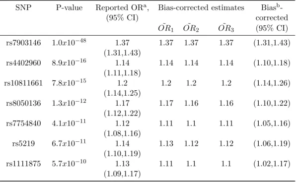
Table 2.3: Original vs. corrected odds ratio estimates for published genetic association study III: GWAS of T2D, Scott et al. (2007) (9521 cases and 12183 controls)
aStandard OR values as reported
bCorrection method proposed in this manuscript
SNP P-value Reported ORa, Bias-corrected estimates Biasb
-(95% CI) corrected
˜
OR1 OR˜ 2 OR˜ 3 (95% CI)
rs7903146 1.0x10−48 1.37 1.37 1.37 1.37 (1.31,1.43) (1.31,1.43)
rs4402960 8.9x10⁻¹⁶ 1.14 1.14 1.14 1.14 (1.10,1.18) (1.11,1.18)
rs10811661 7.8x10⁻¹⁵ 1.2 1.2 1.2 1.2 (1.14,1.26) (1.14,1.25)
rs8050136 1.3x10⁻¹² 1.17 1.17 1.16 1.16 (1.10,1.22) (1.12,1.22)
rs7754840 4.1x10⁻¹¹ 1.12 1.11 1.1 1.11 (1.05,1.16) (1.08,1.16)
rs5219 6.7x10⁻¹¹ 1.14 1.13 1.12 1.12 (1.06,1.19) (1.10,1.19)
2.4
Discussion
We have presented an approach that greatly reduces significance bias for odds ratios in genome association scans, and is much simpler than competing approaches. We favor the use of ˜β3as a general-purpose estimator with fairly uniform MSE as a function ofβ.
However, all of the three corrected estimators have greatly superior performance to the na¨ıve estimator. Although developed for case-control applications, our methodology is an effective blueprint to perform inference whenever a Wald-like statistic has been used to declare significance. Thus the general approach can be used in numerous other settings, including regression-based quantitative trait association analyses. Our results are qualitatively similar to those of other investigators (Yu et al. 2007; Z¨ollner and Pritchard 2007) (e.g., see bias curves similar to ours in Figure 2 of Z¨ollner and Pritchard (2007)). Additional comparisons to these approaches should be performed in future work, although comparison is complicated by differing genetic models. To our knowledge, our approach is the only method that can perform bias correction based only on published summary tables.
discouraging excessive massaging of data and trying various test procedures to achieve genome-wide significance. If a SNP suddenly becomes significant after numerous data manipulation procedures have been applied, its z-statistic is likely to be only slightly above the threshold c. Thus, as we observed in the µ version of the problem, the conditional likelihood estimator will be dramatically shrunk towards the null. Thus the estimated SNP effect size will be very modest, as is appropriate here for a likely spurious finding.
Our current approach does not explicitly consider multi-stage or other sequential designs, in which SNPs meeting a loose standard of significance are used for further testing in a follow-up sample. However, for multistage designs in which almost all SNPs that will eventually be declared significant are carried forward to later stages, the approach may be used directly. Also, our results technically hold for a SNP randomly selected from those achieving the significance threshold, and thus an additional bias may be anticipated for the most highly significant SNPs among a collection of significant SNPs. Although we believe this second source of bias is much less than that produced by significance selection, it is the subject of continuing investigation.
2.5
Web Resources
The URLs for data presented herein are as follows: Online Mendelian Inheritance in Man (OMIM), http://www.ncbi.nlm.nih.gov/Omim/. R code and a simple Ex-cel calculator to perform our method are available at www.bios.unc.edu/~fwright/
genomebias.
-0.6 -0.4 -0.2 0.0 0.2 0.4 0.6 -1 .5 -1 .0 -0 .5 0 .0 0 .5 1 .0 β mea n β ^ β ~ 1 β ~ 2 β ~ 3
-0.6 -0.4 -0.2 0.0 0.2 0.4 0.6
-1 .5 -1 .0 -0 .5 0 .0 0 .5 1 .0 β mea n β^ β ~ 1 β ~ 2 β ~ 3
-0.6 -0.4 -0.2 0.0 0.2 0.4 0.6
0. 0 0. 5 1. 0 1. 5 β ms e β ^ β ~ 1 β ~ 2 β ~ 3
-0.6 -0.4 -0.2 0.0 0.2 0.4 0.6
0. 0 0. 5 1. 0 1. 5 β ms e β^ β ~ 1 β ~ 2 β ~ 3
-0.6 -0.4 -0.2 0.0 0.2 0.4 0.6
-1 .0 -0 .5 0 .0 0 .5 β mea n β ^ β ~ 1 β ~ 2 β ~ 3
-0.6 -0.4 -0.2 0.0 0.2 0.4 0.6
-1 .0 -0 .5 0 .0 0 .5 β mea n β^ β ~ 1 β ~ 2 β ~ 3
-0.6 -0.4 -0.2 0.0 0.2 0.4 0.6
0. 0 0. 1 0. 2 0. 3 0. 4 0. 5 0. 6 0. 7 β ms e β ^ β ~ 1 β ~ 2 β ~ 3
-0.6 -0.4 -0.2 0.0 0.2 0.4 0.6
0. 0 0. 2 0. 4 0 .6 β ms e β^ β ~ 1 β ~ 2 β ~ 3 Model MAF
RECESSIVE ADDITIVE DOMINANT
-0.6 -0.4 -0.2 0.0 0.2 0.4 0.6 -0 .5 0 .0 0 .5 β mea n β ^ β ~ 1 β ~ 2 β ~ 3
-0.6 -0.4 -0.2 0.0 0.2 0.4 0.6
0. 0 0. 1 0. 2 0. 3 0. 4 0. 5 0. 6 β ms e β ^ β ~ 1 β ~ 2 β ~ 3
-0.6 -0.4 -0.2 0.0 0.2 0.4 0.6
-0 .6 -0 .4 -0 .2 0 .0 0 .2 0 .4 0 .6 β mea n β ^ β ~ 1 β ~ 2 β ~ 3
-0.6 -0.4 -0.2 0.0 0.2 0.4 0.6
0. 00 0. 05 0. 10 0. 15 0. 20 β ms e β ^ β ~ 1 β ~ 2 β ~ 3
-0.6 -0.4 -0.2 0.0 0.2 0.4 0.6
-0 .5 0 .0 0 .5 β mea n β^ β ~ 1 β ~ 2 β ~ 3
-0.6 -0.4 -0.2 0.0 0.2 0.4 0.6
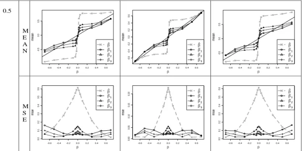
0. 0 0. 1 0. 2 0. 3 0. 4 0. 5 0. 6 β ms e β^ β ~ 1 β ~ 2 β ~ 3 M E A N 0.5 M S E
Figure 2.6: Expected values and mean squared errors for the estimators for the three models.
-0.6 -0.4 -0.2 0.0 0.2 0.4 0.6 0. 7 0 0 .75 0. 8 0 0 .85 0. 9 0 0 .95 1. 0 0 β co ve ra g e
-0.6 -0.4 -0.2 0.0 0.2 0.4 0.6
0. 7 0 0 .75 0. 8 0 0 .85 0. 9 0 0 .95 1. 0 0 β co ve ra g e
-0.6 -0.4 -0.2 0.0 0.2 0.4 0.6
0. 7 0 0 .75 0. 8 0 0 .85 0. 9 0 0 .95 1. 0 0 β co ve ra g e
-0.6 -0.4 -0.2 0.0 0.2 0.4 0.6
0. 7 0 0 .75 0. 8 0 0 .85 0. 9 0 0 .95 1. 0 0 β co ve ra g e
-0.6 -0.4 -0.2 0.0 0.2 0.4 0.6
0. 7 0 0 .75 0. 8 0 0 .85 0. 9 0 0 .95 1. 0 0 β co ve ra g e
-0.6 -0.4 -0.2 0.0 0.2 0.4 0.6
0. 7 0 0 .75 0. 8 0 0 .85 0. 9 0 0 .95 1. 0 0 β co ve ra g e
-0.6 -0.4 -0.2 0.0 0.2 0.4 0.6
0. 7 0 0 .75 0. 8 0 0 .85 0. 9 0 0 .95 1. 0 0 β co ve ra g e Model MAF
RECESSIVE ADDITIVE DOMINANT
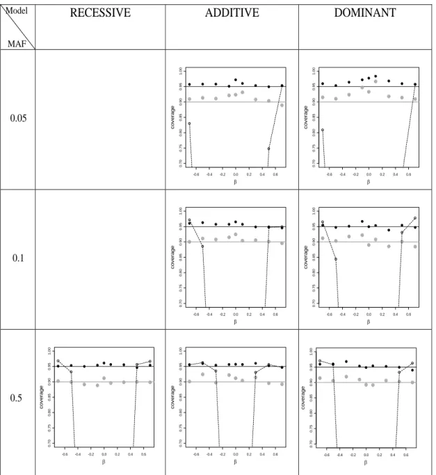
0.05 0.1 0.5
Figure 2.7: Estimates of the CI coverage probability plotted against β for the three genetic models.
samplesize m ean 0 .00 .2 0 .40 .60 .8 β^ β ~ 1 β ~ 2 β ~ 3 beta=0
1000 2000 3000 4000
samplesize ms e β^ β ~ 1 β ~ 2 β ~ 3
1000 2000 3000 4000
0 .0 0 .2 0. 4 0. 6 0. 8 1. 0 samplesize m ean 0 .00 .2 0 .40 .60 .8 β ^ β ~ 1 β ~ 2 β ~ 3 beta=0.18
1000 2000 3000 4000
samplesize ms e β ^ β ~ 1 β ~ 2 β ~ 3
1000 2000 3000 4000
samplesize m ean 0 .00 .2 0 .40 .60 .8 β^ β ~ 1 β ~ 2 β ~ 3 beta=0.34
1000 2000 3000 4000
0 .0 0 .2 0. 4 0. 6 0. 8 1. 0 samplesize ms e β^ β ~ 1 β ~ 2 β ~ 3
1000 2000 3000 4000
0 .0 0 .2 0. 4 0. 6 0. 8 1. 0
Figure 2.8: Expected values and the mean squared errors of the estimators for the additive model with MAF=0.25.
-0.6 -0.4 -0.2 0.0 0.2 0.4 0.6 -0 .6 -0 .4 -0 .2 0 .0 0 .2 0 .4 0 .6 β m e a n
-0.6 -0.4 -0.2 0.0 0.2 0.4 0.6
-0 .6 -0 .4 -0 .2 0 .0 0 .2 0 .4 0 .6 β m e a n β ~ 1 cov β ~ 1
-0.6 -0.4 -0.2 0.0 0.2 0.4 0.6
-0 .5 0 .0 0 .5 β m e a n β^ β ~ 1 β ~ 2 β ~ 3
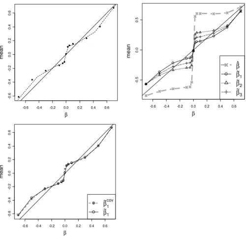
Figure 2.9: Properties of the corrected estimators extended to additional set-tings.
Throughout this figure we use the additive model, MAF=0.25, and n = 1000 except where noted. (a) Expectations of ˜β1 vs. β (plotted points) forn = 1000, overlaid with
Chapter 3
Analysis of Secondary Phenotypes
in Case-control Studies
3.1
Introduction
analysis of a phenotype may come from several GWAS, for which data were originally collected with different research objectives in mind. Because of its efficient design, data for GWAS are usually case-control sampled. In such cases the data cannot be considered as a random sample from the population and ignoring the the ascertainment on the basis of the primary phenotype can produce biased estimate of the association between a SNP and a secondary phenotype (Nagelkerke et al. 1995). For the appropriate analysis of secondary phenotype we have to take into consideration the biased sampling.
sampling mechanism, but the estimates that we derive from each of these methods may be estimating quantities very different from the one that we are interested in. For example, including the disease phenotype as a covariate is a convenient way of incorporating the sampling mechanism in the analysis but not necessarily the true model that we believe in. Monsees et al. (2009) have recently discussed in details the situations under which the na¨ıve analysis that ignores the ascertainment or the analysis that includes disease status as a covariate are valid.
The standard survey approach or Horvitz-Thompson approach uses weights in-versely proportional to the selection probabilities (Jiang et al. 2006; Scott and Wild 2002). Richardson et al. (2007) describe it as a stratum-weighted logistic regression for a binary secondary phenotype and compare its merits with the usual practice of adjust-ing for the disease status by includadjust-ing it in the regression as a covariate. It is, of course, necessary to have knowledge of the sampling fractions for cases and controls, which we do for nested case-control studies. But for population-based case-control studies, this information is not readily available. Rather than focus on the absolute sampling frac-tions, we can try to estimate from external information, such as the prevalence, the ratio of the the sampling fractions which would be sufficient for the purpose of weighted regression.
one needs to model the joint distribution of the primary and the secondary pheno-types given the genotype and other covariates. The joint distribution can be factorized further into the marginal distribution of the secondary phenotype and the conditional distribution of the primary phenotype given the secondary phenotype. Our interest lies in estimating the parameters of the marginal distribution of the secondary phe-notype given the gephe-notype and the covariates. As Jiang et al. (2006) have described, we can either treat the conditional distribution of the primary phenotype given the secondary phenotype non-parametrically or we can model it as a logistic regression. Lin and Zeng (2008) have developed likelihood methods for analysis of both binary and continuous secondary traits where they have modeled the the conditional distribution of the primary phenotype given the secondary phenotype as a logistic regression. An alternative way to specify the joint model is to parametrically model the marginals of the primary and the secondary phenotypes and also build a parametric model for their association given the genotype and the covariates. The distribution of the genotype and the covariates is a nuisance parameter in the retrospective likelihood. It is difficult to parameterize the covariate distribution and is usually treated non-parametrically.
allowed for inclusion of covariates in our models and have performed extensive simu-lations to compare the performance of our proposed approach with the performances of the na¨ıve method of prospectively analyzing the combined sample of cases and con-trols ignoring the biased sampling, case-only analysis, concon-trols-only analysis, and the weighted method.
3.2
Methods
l = logL =
n
X
i=1
logP(Y =yi, G=gi,Z=zi|di)
=
n
X
i=1
logP(D=di, Y =yi|gi,zi;θ) + n
X
i=1
logP(G=gi,Z=zi)
−
n
X
i=1
logP(D =di).
For prospectively collected data, we can make inference about θ fromPn
i=1logP(D=
di, Y =yi|gi,zi;θ) and ignore P(G=g,Z =z). But, for case-control data, we cannot
ignoreP(G=g,Z =z) since it is intertwined with θ in
P(D=d) = X
y
X
g
X
z
P(D=d, Y =y|g,z;θ)P(G=g,Z=z).
The retrospective likelihood, therefore, is a function of θ, the parameter of interest, and P(G = g,Z = z), the nuisance parameter. We assume that disease prevalence is known approximately and incorporate that information in the likelihood. Under known prevalence, sayP(D= 1) = Π, we maximize
l =
n
X
i=1
logP(D=di, Y =yi|gi,zi;θ) + n
X
i=1
with respect to (θ, P(G=g,Z=z))0 subject to the constraint
X
y
X
g
X
z
P(D= 1, Y =y|g,z;θ)P(G=g,Z=z) = Π. (3.1)
We assume that G and Z are independent in the population. Since G is discrete and can take at most three values, we treat the probability distribution of G, p(g), as a nuisance parameter and maximize the likelihood with respect to it, subject to the constraint P
gp(g) = 1. It is generally difficult and unreasonable to parameterize the
covariate distribution P(Z = z). If all the covariates are categorical and there are tractable number of combinations of the levels of the covariates, then we can treat them as nuisance parameters and maximize the likelihood with respect to them. For illustration purpose, let us consider the situation where the genotype is coded as 0 or 1 with P(G = 1) = δ and we have a single binary covariate, Z, with probability of success ψ. Then we maximize
l(θ, δ, ψ) =
n
X
i=1
logP(D=di, Y =yi|gi,zi;θ) +nG1logδ
+(1−nG1) log (1−δ) +nZ1logψ+ (1−nZ1) log (1−ψ), (3.2)
where nG1 =
n
X
i=1
gi and nZ1 =
n
X
i=1
zi ,
matrix of the MLE can be consistently estimated by the inverse of the observed informa-tion matrix. This method becomes infeasible very quickly as the number of covariates increases and it does not allow for continuous covariates. For continuous covariates we can assume the profile likelihood approach (Lee et al. 1997; Wild 1991; Lin and Zeng 2008; Scott and Wild 2001b). Suppose Z is now a continuous covariate. We have n parameters P(Z = zi) =pi, i = 1, . . . , n describing the distribution of Z. To get the
maximum likelihood estimate of θ we need to maximize
l(θ, δ, p1, . . . , pn) = n
X
i=1
logP(D=di, Y =yi|gi,zi;θ)
+
n
X
i=1
logP(G=gi) + n
X
i=1
logpi
with respect to (θ, δ, p1, . . . , pn)0 subject to the constraints
Pn
i=1pi = 1 and
X
y
1
X
g=0
n
X
i=1
P(D= 1, Y =y|g, zi;θ)P(G=g)pi = Π.
Using Lagrange multipliers, we maximize
l(θ, δ, pi, . . . , pn)
=
n
X
i=1
logP(D=di, Y =yi|gi,zi;θ)
+
n
X
i=1
logP(G=gi) + n
X
i=1
logpi+λ1(
n
X
i=1
pi−1)
+λ2
X
y
1
X
g=0
n
X
i=1
P(D= 1, Y =y|g, zi;θ)P(G=g)pi−Π
!
with respect to (θ, δ, pi, i= 1, . . . , n)0. λ1 and λ2 are determined using the constraints.
Maximizing(3.3) with respect topi we get,
1 pi
−λ1−λ2
X
y
1
X
g=0
P(D= 1, Y =y|g, zi;θ)P(G=g) = 0. (3.4)
Multiplying the above equation by pi on both sides and then taking a sum over i we
get,
λ1 =n−λ2Π.
Substitutingλ1 in (3.4), we have
pi = n−λ2Π +λ2
X
y
1
X
g=0
P(D= 1, Y =y|g, zi;θ)P(G=g)
!−1 .
Thus, the profile log-likelihood for (θ, δ)0 is
lprof ile(θ, δ) = n
X
i=1
logP(D=di, Y =yi|gi,zi;θ) + n
X
i=1
logP(G=gi)
−
n
X
i=1
log n−λ2Π +λ2
X
y
1
X
g=0
P(D= 1, Y =y|g, zi;θ)P(G=g)
! ,
whereλ2 is determined by
n
X
i=1
n−λ2Π +λ2
X
y
1
X
g=0
P(D= 1, Y =y|g, zi;θ)P(G=g)
The estimates from the profile likelihood are consistent and asymptotically normal and the covariance matrix can be consistently estimated by the inverse of the observed information matrix obtained from the profile likelihood. We propose an alternative approach that has been used in various contexts: the pseudo likelihood idea put forward by Gong and Samaniego (1981) for parametric inference and later extended by Hu and Lawless (1997) to a semiparametric setting. The idea involves maximizing the pseudo likelihood Lp
θ, p(g),Pˆ(Z=z)
, where ˆP(Z = z) is a nonparametric estimate of P(Z =z). Under known prevalence the pseudo log-likelihood lp is
lp = logLp
θ, p(g),Pˆ(Z=z) =
n
X
i=1
logP(D=di, Y =yi|gi,zi;θ) + n
X
i=1
logP(G=gi)
along with the constraint
X
y
X
g
X
z
P(D= 1, Y =y|g,z;θ)P(G=g) ˆP(Z =z) = Π.
Noting that
P(Z =z) = P(Z=z|D= 1)P(D= 1) +P (Z =z|D= 0)P(D= 0),
we estimate P (Z=z) by
ˆ
where ˆP (Z=z|D=i) , i = 0,1 are valid estimates being the empirical cumulative distribution functions based on the controls and the cases respectively. For ˆP(D = 1) we have to depend on external information. The pseudo maximum likelihood esti-mate(MLE) is then obtained by maximizing the pseudo log-likelihood,lp,with respect
to the parameter of interest, θ, and the nuisance parameter, p(g). A rigorous devel-opment of the the asymptotic properties of the pseudo MLE is complicated. Hu and Lawless (1997) discuss the asymptotics for pseudo likelihood methods in the context of response-related missing covariates. Following the same lines we plan to lay down the details of the asymptotic theory for pseudo likelihood estimation in our situation. We now discuss how to parameterize the joint distribution (D, Y|g,z) for binary and continuous secondary phenotypes.
3.2.1
Binary secondary phenotype
logit P(D= 1|g,z) = α1+β1g+γ10z
logit P(Y = 1|g,z) =α2+β2g+γ20z
logOR(D, Y |g) = P(D= 1, Y = 1 |g,z)P(D= 0, Y = 0 |g,z)
P(D= 1, Y = 0 |g,z)P(D= 0, Y = 1 |g,z) =α3+β3g .
The pseudo log-likelihood is, therefore, a function ofθ = (α1, β1,γ1, α2, β2,γ2, α3, β3)
0
, the parameter of interest, and p(g), the nuisance parameter. With fixed disease preva-lence, the identity
P(D= 1) =X
z
X
g
exp(α1+β1g+γ10z)
1 + exp(α1+β1g+γ10z)
p(g) ˆP(Z=z) (3.5)
is used to computeα1 given (β1,γ1, α2, β2,γ2, α3, β3)
0
and p(g). Thus, the retrospective pseudo log-likelihood, under known prevalence, is
lp = n
X
i=1
logP(D=di, Y =yi|gi,zi) + n
X
i=1
logP(G=gi),
which is a function of θ = (β1,γ1, α2, β2,γ2, α3, β3,γ3)
0
, and p(g). We obtain the pseudo MLE of θ by maximizing lp with respect to (θ, p(g))0. We can write down
probabilitiesπi. =P(D=i|g,z) andπ.j =P(Y =j|g,z), and the odds ratioψ = π11π00 π10π01,
π11=
1
2(ψ−1)
−1na−p
(a2+b) o
, ψ 6= 1
π1.π.1 , ψ = 1,
wherea= 1 + (π1.+π.1)(ψ−1) and b =−4ψ(ψ−1)π1.π.1. The rest of the πijs can be
derived from π11 and the marginals.
3.2.2
Continuous secondary phenotype
For continuous Y, we consider joint models for (D, Y|g,z) such that the marginal distribution of D given g and z follows a logistic regression model and the marginal distribution ofY given g and z is normal, that is,
logit P(D= 1|g,z) = α1+β1g+γ10z
and Y |g,z∼N α2+β2g+γ20z, σ22
.
We introduce two levels of latency to come up with a joint model which satisfies the above conditions. We assume that the disease status variable, D, is derived from thresholding a latent continuous variable, U, whose marginal density given g and z is logistic with location parameter µ1 =α1+β1g+γ10z and scale parameter 1, that is,
pU|G,Z(u|g,z) = exp (−(u−µ1)) (1 + exp (−(u−µ1)))2
and D=
1, U ≥0 0, U <0
.
⇒P(D= 1 |g,z) = exp (µ1) 1 + exp (µ1)
.
In order to connectU with Y we introduce another latent variableV. We assume that U is derived by transforming a continuous variable, V, whose marginal distribution given g and z is normal with mean µ1 and variance 1, and that (V, Y|g,z) follows
bivariate normal. The required transformation is U = µ1 + log
Φ(V−µ1)
1−Φ(V−µ1). Thus, we
specify the following population model for the bivariate response (D, Y|g,z),
V Y
g,z∼N µ1 µ2 ,
1 ρσ2
ρσ2 σ22
, where
µ1 =α1+β1g+γ10z, µ2 =α2+β2g+γ20z, andρ=α3+β3g .
LetU =µ1+ log Φ(V
−µ1)
1−Φ(V−µ1) and D=
1, U ≥0 0, U < 0
.
Assuming disease prevalence to be known, the retrospective pseudo log-likelihood is a function of θ= (β1,γ1, α2, β2,γ2, σ2, α3, β3)
0
, and p(g),
lp = n
X
i=1
logP(D=di, Y =yi|gi,zi) + n
X
i=1