Motley_unc_0153D_18103.pdf

(1)

CONTROL OF LATERAL ELECTRON TRANSFER BETWEEN COMPOUNDS ANCHORED TO SEMICONDUCTOR INTERFACES

Tyler Chase Motley

A dissertation submitted to the faculty of the University of North Carolina at Chapel Hill in partial fulfillment of the requirements for the degree of Doctor of Philosophy in the

Department of Chemistry (Inorganic).

Chapel Hill 2018

(2)

(3)

ABSTRACT

Tyler Chase Motley: Control of Lateral Electron Transfer between Compounds Anchored to Semiconductor Interfaces

(Under the direction of Gerald J. Meyer)

The need for a clean and renewable energy source is paramount to long term global economic and energy security and is the motivation for this work. The sun is one of the largest sources of renewable energy available. Dye-sensitized solar and photoelectrochemical cells that capture solar energy and convert it to either electricity or solar fuels provide an opportunity to investigate the relevant, molecular, reaction chemistry in such devices. One electron transfer pathway in both devices is lateral electron transfer between compounds anchored to the interface of the metal oxide films. The focus of this dissertation is to understand how structural changes to these compounds influence lateral electron transfer rates. The basic operating principles of dye-sensitized technologies and the relevant background to lateral electron transfer kinetics are given in Chapter 1.

Chapters 2-4 explore the effect of molecular structure on lateral electron transfer kinetics. In Chapters 2 and 3, the effect of 4 and 4′ substituents are examined using a series of compounds of the type [Ru(R2bpy)2(bpy’)]2+_{, where R2bpy was a} 4,4′-substituted-2,2′-bipyridine and bpy’ was a 2,2′-bipyrdine with either carboxylic or phosphonic acid binding

(4)

substituted-triphenylamine donor connected by a thiophene bridge, are anchored to the TiO2 interface and lateral intermolecular electron transfer is studied. This study shows that the intramolecular electronic coupling influences lateral charge transport rates.

(5)

(6)

ACKNOWLEDGEMENTS

There are many people in my life to whom I am eternally grateful for facilitating my personal growth and for fanning the flames of curiosity.

First and foremost, I am indebted to my parents, Douglas and Terri, for being steadfast anchors throughout the roller-coaster that has been graduate school (and life). They have been constant sources of encouragement and strength, and they continue to remind me to “remember your roots.” I am grateful to my brother, Stuart, and my two wonderful nieces, Miley Rae and

Allyson Grace, who remind me not to take myself too seriously and to continue to find joy in the small things. My grandparents, Edna Johnson and Ethel and Lewis Motley, always encouraged me to be the best that I could be and to always keep learning, lessons that I am thankful for. I am also grateful for the rest of my family who are too numerous to list here and who each hold a special place in my heart.

Second, I want to thank Dr. Jerry Meyer for being a great boss and a wonderful mentor over the past five years and encouraging me to be the scientist I have become. I would also like to say a special thank you to Dr. Alexander Miller who allowed me to work in his laboratory for several months while Jerry’s lab transitioned from Johns Hopkins to UNC.

(7)

J. Barr, Dr. Evan E. Beauvilliers, Dr. Brian N. DiMarco, Catherine G. Burton, Andrew B. Maurer, Eric J. Piechota, Matthew D. Brady, Victoria K. Davis, Erica M. James, Sara A. M. Wehlin, Rachel Bangle, Yuting F. Lin, and Michael D. Turlington, for your help and friendship over the past five years.

I would be remiss if I did not thank all of my friends here at UNC Chapel Hill for making this an enjoyable experience. I am especially grateful for my fellow cohort and dear friend, Dr. Wesley B. Swords, with whom I have been on this journey and who has been a constant source of encouragement and friendship. I also owe a special thank you to Erika Van Goethem who was always willing to listen to me vent about research and life. To the both of you, I say thanks, and I look forward to see where life leads you both. Thanks to my fellow teammates on the Dallas Cp Stars, Spring 2014 and 2018 co-rec intramural champions, for teaching me about hockey and being great people to be with both on the court and off. So, to Jake Green, Cortney Cavanaugh, Tony Carestia, and many others, thank you for being wonderful people.

(8)

TABLE OF CONTENTS

LIST OF FIGURES ... xiv

LIST OF TABLES ... xxii

LIST OF SCHEMES... xxiii

CHAPTER 1: Strategies for Solar Energy Conversion and Storage and the Role of Lateral Charge Transport ... 1

1.1 Energy Supply and Demand: A Precarious Balancing Act ... 1

1.1.1 Current Energy Trends: The Case against Fossil Fuels ... 1

1.1.2 A Brighter Tomorrow: The Case for Solar Energy ... 4

1.2 The Photophysics of RuII Polypyridyl Compounds ... 8

1.3 Dye-Sensitized Technologies ... 14

1.3.1 Dye-Sensitized Solar Cells... 14

1.3.2 Dye-Sensitized Photoelectrochemical Cells ... 18

1.4 Lateral Electron Transfer at Semiconductor Interfaces ... 20

1.4.1 Introduction to Marcus Theory ... 21

1.4.2 Mechanism and Experimental Approaches for Lateral Electron Transfer ... 25

1.4.2.1 Quantifying Lateral Electron Transfer through Electrochemistry ... 28

1.4.2.2 Transient Absorption Spectroscopy to Quantify Lateral Electron Transfer Kinetics ... 31

1.4.3 Structural and Solvent Effects on Lateral Electron Transfer ... 33

1.4.4 Effects of Lateral Electron Transfer in DSSCs and DSPECs ... 38

1.5 Conclusion ... 41

(9)

CHAPTER 2: A Distance Dependence to Lateral Self-Exchange across Nanocrystalline TiO2. A Comparative Study of Three Homologous RuIII/II

Polypyridyl Compounds ... 56

2.1 Introduction ... 56

2.2 Experimental Methods ... 61

2.2.1 Materials ... 61

2.2.2 Synthesis of [Ru(dmb)2(deeb)](PF6)2 (1) ... 61

2.2.3 Synthesis of [Ru(dmb)2(dcbH2)](PF6)2 (dmb) ... 62

2.2.4 Thin Film Preparation ... 63

2.2.5 UV-Visible Spectroscopy ... 63

2.2.6 Electrochemistry ... 64

2.2.7 Data Analysis ... 65

2.2.8 Calculation of c0 and R ... 66

2.3 Results ... 68

2.4 Discussion ... 76

2.4.1 Quantification of Reduction Potentials and Apparent Diffusion Coefficients ... 77

2.4.2 Self-Exchange Kinetics and Theory ... 80

2.5 Conclusions ... 82

2.6 Acknowledgements ... 83

2.7 Additional Content ... 84

2.6.1 Single Crystal X-ray Crystallography ... 85

REFERENCES ... 88

CHAPTER 3: Influence of 4 and 4′ Substituents on RuIII/II Polypyridyl Self-Exchange Electron Transfer across Nanocrystalline TiO2 Surfaces ... 91

(10)

3.2.1 Materials ... 96

3.2.2 Preparation of Thin Films ... 96

3.2.3 Spectroscopy ... 97

3.2.4 Chronoabsorptometry... 97

3.3 Results ... 98

3.4.1 Quantification of Reduction Potentials and Apparent Diffusion Coefficients ... 106

3.4.2 Substituent Effects on Self-Exchange Electron Transfer at the Interface ... 109

REFERENCES ... 117

CHAPTER 4: Intramolecular Electronic Coupling Enhances Lateral Electron Transfer across Semiconductor Interfaces ... 122

4.2.1 General Information ... 124

4.2.2 Preparation of TiO2 Thin Films ... 124

4.3 Results and Discussion ... 126

4.4 Conclusion ... 131

(11)

REFERENCES ... 134

CHAPTER 5: Thermal Bimolecular Electron Transfer in the Marcus Inverted Region: Exploiting Nonadiabatic Electron Transfer ... 137

5.2.1 Materials ... 139

5.2.2 General Procedure for the Synthesis of [Ru(R2bpy)2Cl2] ... 140

5.2.3 General Procedure for the Synthesis of the Cobalt Compounds ... 140

5.2.4 Synthesis of [Ru(dtb)2(dab)](PF6)2 ... 141

5.2.5 Synthesis of [Ru(dtb)2(mab)](PF6)2 ... 141

5.2.6 Synthesis of [Ru(MeObpy)2(dmeb)](PF6)2 ... 142

5.2.7 Synthesis of [Ru(dmb)2(dmeb)](PF6)2 ... 143

5.2.8 Synthesis of [Ru(Fbpy)2(dcb)](PF6)2 ... 143

5.2.9 Synthesis of [Ru(Fbpy)2(dmeb)](PF6)2 ... 144

5.2.10 Synthesis of [Ru(Brbpy)2(dmeb)](PF6)2 ... 144

5.2.11 Synthesis of [Ru(btfmb)2(dmeb)](PF6)2 ... 145

5.2.12 Nuclear Magnetic Resonance Spectroscopy (NMR) ... 146

5.2.13 Electrospray Ionization Mass Spectrometry (ESI-MS) ... 146

5.2.14 Spectroscopy ... 147

5.2.15 Spectroelectrochemistry ... 148

5.3 Results and Discussion ... 149

(12)

CHAPTER 6: Excited-State Decay Pathways of Tris(bidentate)

Cyclometalated Ruthenium(II) Compounds ... 167

6.2.1 Materials ... 170

6.2.2 General Procedure for the Synthesis of [Ru(C^N)(CH3CN)4](PF6) ... 171

6.2.3 Synthesis of [Ru(ppy)(CH3CN)4](PF6) ... 171

6.2.4 Synthesis of [Ru(ppyF2)(CH3CN)4](PF6) ... 171

6.2.5 Synthesis of [Ru(ppyCF3)(CH3CN)4](PF6) ... 172

6.2.6 Synthesis of [Ru(deeb)2(ppy)](PF6) ... 172

6.2.7 Synthesis of [Ru(bpy)2(ppy)](PF6) ... 173

6.2.8 Synthesis of [Ru(dtb)2(ppy)](PF6) ... 173

6.2.9 Synthesis of [Ru(MeObpy)2(ppy)](PF6) ... 174

6.2.10 Synthesis of [Ru(deeb)2(ppyF2)](PF6) ... 174

6.2.11 Synthesis of [Ru(bpy)2(ppyF2)](PF6) ... 175

6.2.12 Synthesis of [Ru(MeObpy)2(ppyF2)](PF6) ... 176

6.2.13 Synthesis of [Ru(bpz)2(ppyCF3)](PF6) ... 176

6.2.14 Synthesis of [Ru(deeb)2(ppyCF3)](PF6) ... 177

6.2.15 Synthesis of [Ru(bpy)2(ppyCF3)](PF6) ... 178

6.2.16 Synthesis of [Ru(MeObpy)2(ppyCF3)](PF6) ... 178

6.2.17 Nuclear Magnetic Resonance Spectroscopy (NMR) ... 179

6.2.18 Electrospray Ionization-Mass Spectrometry (ESI-MS) ... 179

6.2.19 Elemental Analysis (EA) ... 180

6.2.20 Square Wave Voltammetry ... 180

(13)

6.2.22 Steady-State Photoluminescence and Quantum Yield

Determination ... 181

6.2.23 Temperature-Dependent, Time-Resolved Photoluminescence ... 181

6.2.24 Single-Mode, Franck-Condon Lineshape Analysis ... 182

6.2.25 Time-Correlated Single Photon Counting ... 182

6.2.26 Arrhenius Analysis ... 183

6.3 Results ... 183

6.4.1 Effects of Ligand Substitution ... 195

6.4.2 Excited-State Characterization and the Energy Gap Law ... 196

6.4.3 Arrhenius Analysis ... 201

(14)

LIST OF FIGURES

Figure 1.1. Historical average atmospheric CO2 concentrations as measured from the Vostok ice core samples in Antarctica (black ■, taken from ref. 23_{) or}

from atmospheric samples taken at the South Pole (red ●, taken from ref. 24). ... 3

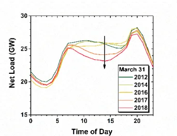
Figure 1.2. Net load reported by the California Independent System Operator (CA ISO) on the California electrical grid for March 31st of the specified years. The increasing contribution of photovoltaic solar energy production is

decreasing the afternoon demand as indicated by the black arrow.44 ... 6

Figure 1.3. (A) A simple molecular orbital diagram for [Ru(bpy)3](PF6)2 in a pseudo-octahedral (Oh) geometry. In this diagram, the gray orbital sets indicate orbitals that are predominantly located on the 2,2′-bipyridine ligands and the black orbital sets indicate those that are primarily Ru-based. Some of the resulting molecular orbitals are omitted for clarity. Also depicted, are the common electronic transitions that are observed in the UV-visible electronic spectrum. (B) UV-visible electronic and the normalized photoluminescence

spectra of [Ru(bpy)3](PF6)2 acquired at room temperature in neat acetonitrile. ... 9

Figure 1.4. A Jablonski-type diagram for the [Ru(bpy)3](PF6)2 in acetonitrile. The 1GS is referenced to the E°(RuIII/II) of the compound. The energy of the 1_{MLCT and}3_{MLCT states were determined from the energy of the peak in the} UV-visible and photoluminescence spectra, respectively. The illustrated LF and fourth 3MLCT energies are the activation energies for crossing from the 3MLCT

state. Intersystem crossing is abbreviated as ISC. ... 11

Figure 1.5. The standard solar irradiance (AM 1.5 Standard88) measured on the surface of the Earth. The total area under the curve represents the amount of power per unit area that strikes the surface. The gray shaded box and the diagonal-filled box represents the photons with the appropriate energy for

bandgap excitation of silicon and anatase TiO2, respectively... 14

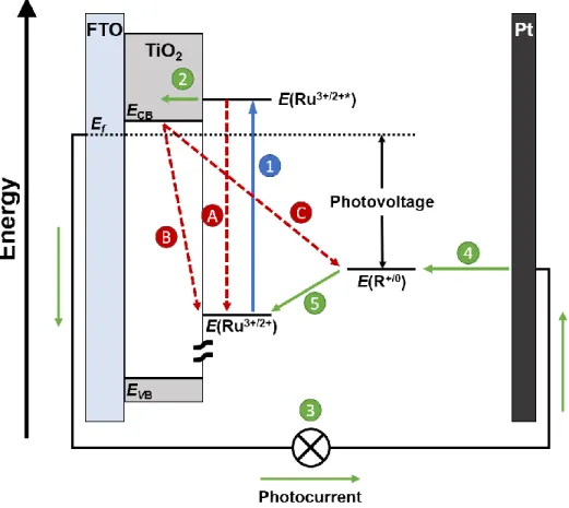
Figure 1.6. A schematic representation of an n-type DSSC using a generic RuII polypyridyl chromophore (Ru) and redox mediator (R). The favorable processes in the DSSC, in order, are (1) photoexcitation, (2) electron injection into the conduction band of TiO2, (3) movement through the external circuit to perform work, (4) reduction of the redox mediator, (5) regeneration of the oxidized Ru sensitizer. Nonproductive pathways include (A) excited-state relaxation, (B) back-electron transfer, and (C) charge recombination all of

which result in a loss of device efficiency. ... 16

(15)

oxidized dye reaches the WOC and is regenerated (4). Once the WOC has been oxidized four times, it oxidizes water (5). H2 generation, a two-electron process, occurs at the Pt electrode (6). Nonproductive pathways include (A) excited-state relaxation, (B) back-electron transfer, and (C) charge recombination all of

which result in a loss of device efficiency. ... 19

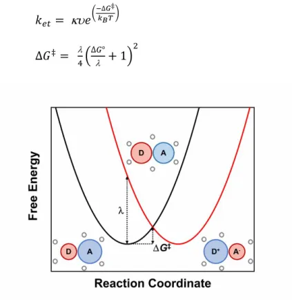
Figure 1.8. One-dimensional potential energy surfaces for the nonadiabatic, self-exchange electron transfer between an electron donor, D, and an electron acceptor, A. The reactant (black) and product (red) potential surfaces are represented as harmonic oscillators. Depicted is the structure of the encounter complex and inner-solvation sphere before, during, and after electron transfer. Indicated on the graph is the reorganization energy, , and the Gibbs free energy

of activation, ΔG‡_{. ... 22}

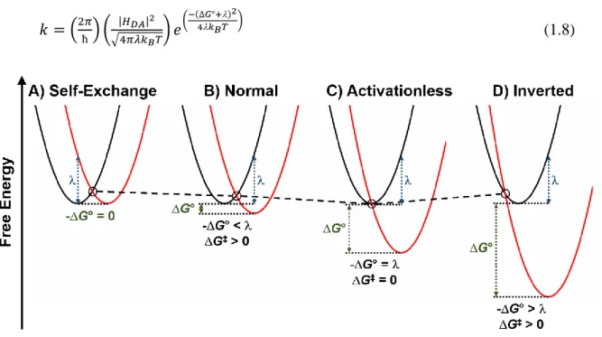
Figure 1.9 One-dimensional potential energy surfaces depicting regimes of electron transfer predicted by nonadiabatic Marcus theory: (A) self-exchange electron transfer (Marcus normal) (B) Marcus normal region, (C) activationless region, and (D) Marcus inverted region. The reactant (black) and product (red) potential energy surfaces are depicted as harmonic oscillators. The crossing point for each regime is highlighted to emphasize the change between the three regimes. The reorganization energy (blue) and the Gibbs free energy of the

reaction (green) are also depicted. ... 23

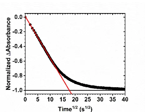
Figure 1.10. A typical Anson plot of the normalized change in absorbance as a function of the square root of time following a potential step sufficiently positive of the formal reduction potential of the surface-anchored compound. The red line is a fit to the Anson equation, eq 1.13, for the initial absorbance

change. ... 29

Figure 1.11. (A) An idealized TiO2 nanoparticle sensitized with and RuII polypyridyl compounds with the lowest-energy transition dipole moment depicted by the black arrow. Given the electric field vector of the linearly-polarized laser pulse, the probability that an incident photon would excite the chromophore is given. (B) The time evolution an idealized TiO2 nanoparticle

after photoexcitation with linearly-polarized laser pulse. ... 32

Figure 1.12. A depiction of the “dry cell” dye-sensitized solar cell which used lateral self-exchange electron transfer between the oxidized chromophore to complete the circuit rather than a redox mediator in solution. Photoexcitation leads to electron injection on the sensitized TiO2 interface, and the electrons are collected at the FTO. Lateral self-exchange electron transfer shuttle the

oxidizing equivalent to the Pt counter electrode. ... 39

(16)

after electron transfer. The blue spheres depict counterions and exaggerates

their location and movement during the electron transfer process. ... 59

Figure 2.2. (a) Crystal structure of [Ru(dmb)2(deeb)](PF6)2. b) Crystal structure of [Ru(dtb)2(dcbH2)](ClO4)2. All hydrogen atoms and anions are omitted for

clarity purposes. Color code: Pink, Ru; blue, N; red, O; gray, C. ... 69

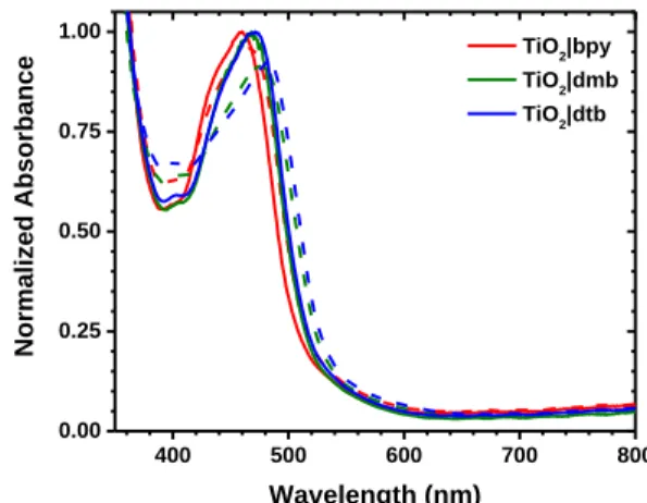
Figure 2.3. Normalized absorption spectra of compounds bpy, dmb, and dtb

anchored to TiO2 in neat CH3CN (solid line) or in a 0.1 M LiClO4 solution in CH3CN (dashed line). The TiO2 absorption spectrum was subtracted out from

the spectra of the surface-functionalized films. ... 70

Figure 2.4. Spectroelectrochemical oxidation of TiO2|dmb immersed in 0.1 M LiClO4/CH3CN electrolyte. The inset plots the fraction of oxidized or reduced compound as a function of applied potential. Overlaid is a fit to a modified

Nernst equation, eq 2.5. ... 71

Figure 2.5. Normalized absorption change measured after application of a potential sufficient to oxidize the indicated compounds plotted against the

square root of time. Overlaid in gold is the fit based on eq 2.6. ... 73

Figure 2.6. Representative cyclic voltammograms for dmb anchored to TiO2

immersed in 0.1 M LiClO4 in CH3CN at the indicated temperatures. ... 74

Figure 2.7. (A) Arrhenius plot for bpy, dmb, and dtb anchored to TiO2 describing the variation of DCV with inverse temperature as obtained by cyclic voltammetry. Overlaid are the best fits to the Arrhenius equation. (B) The temperature dependence of kSE as described by nonadiabatic Marcus theory

(overlaid curves). ... 76

Figure 2.8. The temperature dependence of kSE with fits to non-adiabatic Marcus theory (overlaid curves) calculated with three different values of R for

TiO2|dmb. ... 84

Figure 2.9. UV-visible spectra generated during the oxidation of bpy.

Conversion from RuII_{to Ru}III_{proceeds from purple to red. ... 84}

Figure 2.10. UV-visible spectra generated during the oxidation of dtb.

Conversion from RuII to RuIII proceeds from purple to red. ... 85

Figure 3.1. The normalized UV-visible absorbance spectra for each [Ru(R2bpy)2(P)]|TiO2 film submerged in CH3CN solutions containing 0.1 M

LiClO4 with an unsensitized thin film as a reference. ... 99

(17)

to grow in centered at 675 nm. The inset shows the normalized absorbance change plotted against the square root of time. The data were fit to the Anson

equation through the first 60% of the total absorbance change (red line). ... 101

Figure 3.3. The normalized change in absorbance after the application of sufficiently positive potential to oxidize the [Ru(R2bpy)2(P)]|TiO2 plotted as a

function of the square root of time for all compounds used in this study. ... 102

Figure 3.4. The variation of the measured apparent diffusion coefficients (DCA) for [Ru(bpy)2(P)]|TiO2 with the fractional surface coverage (Γ/Γ0), where Γ0 was the maximum surface coverage attained in the most concentrated dyeing solution (5 mM). The DCA were measured in CH3CN solutions with 0.1 M

LiClO4 electrolyte. Error bars for DCA included for all data. ... 103

Figure 3.5. The dependence of the measured E1/2(RuIII/II) (black, ■) and of log(kH/kR) (red, ●) on the summative Hammett parameter, σT, for all [Ru(R2bpy)2(P)]|TiO2. The measured E1/2(RuIII/II) displayed a strong correlation with σT with a slope of 0.09 V vs NHE. No such correlation was observed with

log(kH/kR). Error bars are given for the log(kH/kR) data. ... 106

Figure 3.6. The dependence of the saturation surface coverage, Γ, with the steric size of the substituent in the 4 and 4′ positions of [Ru(R2bpy)2(P)]|TiO2

as given by the Charton value. Error bars are included for the measured Γ0. ... 111

Figure 3.7. The RuIII/II lateral self-exchange electron transfer rate constant versus the difference intermolecular distance, δ. The distance was varied by either (A, black ■) changing the steric size of the -R group at the 4 and 4′ positions (β = 1.2 ± 0.2 Å-1_{) or (B, red ●) functionalizing the TiO2 with} [Ru(bpy)2(P)]2+ from dilute dying solutions (β = 1.18 ± 0.09 Å-1). Error bars are

given for the ln(kR). ... 112

Figure 3.8. The UV-visible spectral changes after the application a potential sufficient to oxidize [Ru(MeObpy)2(P)]|TiO2. A bleach of the characteristic MLCT transition was observed at 480 nm as the film was oxidized from RuII to RuIII_{. A new peak associated with the Ru}III_{species was observed to grow in} centered at 550 nm. The inset shows the normalized absorbance change plotted against the square root of time. The data were fit to the Anson equation through

the first 60% of the total absorbance change (red line). ... 114

Figure 3.9. The UV-visible spectral changes after the application a potential sufficient to oxidize [Ru(dmb)2(P)]|TiO2. A bleach of the characteristic MLCT transition was observed at 465 nm as the film was oxidized from RuII to RuIII. A new peak associated with the RuIII_{species was observed to grow in centered} at 675 nm. The inset shows the normalized absorbance change plotted against the square root of time. The data were fit to the Anson equation through the first

(18)

Figure 3.10. The UV-visible spectral changes after the application a potential sufficient to oxidize [Ru(bpy)2(P)]|TiO2. A bleach of the characteristic MLCT transition was observed at 455 nm as the film was oxidized from RuII to RuIII. A new peak associated with the RuIII species was observed to grow in centered at 700 nm. The inset shows the normalized absorbance change plotted against the square root of time. The data were fit to the Anson equation through the first

60% of the total absorbance change (red line). ... 115

Figure 3.11. The UV-visible spectral changes after the application a potential sufficient to oxidize [Ru(Brbpy)2(P)]|TiO2. A bleach of the characteristic MLCT transition was observed at 465 nm as the film was oxidized from RuII to RuIII_{. A new peak associated with the Ru}III_{species was observed to grow in} centered at 700 nm. The inset shows the normalized absorbance change plotted against the square root of time. The data were fit to the Anson equation through

Figure 3.12. The UV-visible spectral changes after the application a potential sufficient to oxidize [Ru(btfmb)2(P)]|TiO2. A bleach of the characteristic MLCT transition was observed at 440 nm as the film was oxidized from RuII to RuIII_{. A new peak associated with the Ru}III_{species was observed to grow in} centered at 740 nm. The inset shows the normalized absorbance change plotted against the square root of time. The data were fit to the Anson equation through

Figure 4.1. The UV-visible absorption spectra for (A) 1x, (B) 1p, (C) 2x, and (D) 2p obtained after a potential step at time zero initiated the oxidation of the indicated compounds anchored to TiO2 thin films immersed in a 0.1 M LiClO4 solution in CH3CN. The absorption decrease in the 400-600 nm region reported primarily on the RuII oxidation while the growth in the 650-800 nm region

reported primarily on the TPA0 oxidation. ... 126

Figure 4.2. The normalized change in absorbance as a function of the square root of time measured after the application of a potential sufficient to oxidize

both the TPA0 to TPA+ (A) and RuII to RuIII (B). ... 128

Figure 4.3. The normalized change in absorbance plotted against the square root of time for 1x (A) and 1p (B) monitored at 525 nm (RuIII/II) and 750 nm (TPA+/0). Overlaid are the lines of best fit to the Anson equation for each set of

kinetic data through the initial 60% of the total change. ... 132

Figure 4.4. The normalized change in absorbance plotted against the square root of time for 2x (A) and 2p (B) monitored at 525 nm (RuIII/II) and 750 nm (TPA+/0). Overlaid are the lines of best fit to the Anson equation for each set of kinetic data through the initial 60% of the total change. For 2p, the RuIII/II oxidation kinetics were also fit after the “induction” period (t1/2_{> 1.25 s}1/2_{) and}

(19)

Figure 5.1. Spectroelectrochemical oxidation of [Ru(dtb)2(dmeb)](PF6)2 in a CH3CN solution containing 0.1 M LiClO4. The inset shows the mole fraction of the Ru2+ and Ru3+ compounds as a function of the applied potential. Overlaid

is a fit to the modified Nernst equation, eq 5.2. ... 151

Figure 5.2. Spectroelectrochemical oxidation of [Co(bpy)3](PF6)2 in a CH3CN solution containing 0.1 M LiClO4. The inset is a cyclic voltammogram obtained for [Co(bpy)3](PF6)2 in 0.1 M LiClO4/CH3CN solutions at a scan rate of 0.1 V/s.

... 152

Figure 5.3. (A) Nanosecond transient kinetic data acquired for a CH3CN solution containing only [Ru(dtb)2(dmeb)](PF6)2 (black, exc, 488 nm; probe, 520 nm) or only [Co(bpy)3](PF6)2 (red, exc, 488 nm; probe, 470 nm). Overlaid in blue is a single-exponential fit for the excited-state decay of [Ru(dtb)2(dmeb)](PF6)2. (B) Nanosecond transient kinetic data acquired for an acetonitrile solution containing 2.510-5, 110-4, and 2.510-3 M of [Ru(dtb)2(dmeb)](PF6)2, [Co(bpy)3](PF6)2, and [Co(bpy)3](PF6)3, respectively (exc, 488 nm; probe, 495 nm; laser fluence, 4.8 mJ/pulse). Overlaid in red is a

fit to pseudo-first order kinetics. ... 154

Figure 5.4. The dependence of the back-electron transfer rate constant, ket, on the driving force, ΔG°. Overlaid are the fits to the nonadiabatic Marcus equation, eq 5.1. The electronic coupling matrix element, HDA, was a shared parameter during the fitting process and was found to be 0.02 ± 0.001 meV. The reorganization energies, , were found to be 1.1 ± 0.1 eV and 1.4 ± 0.1 eV for the back-electron transfer reactions with [Co(bpy)3]2+ and [Co(dmb)3]2+,

respectively. ... 158

Figure 6.1. Square wave voltammogram for [Ru(bpy)2(ppy)]+ in an CH3CN

solution containing 0.1 M LiClO4 at room temperature. ... 186

Figure 6.2. The UV-visible absorption (solid) and photoluminescence (dashed) spectra of (A) [Ru(deeb)2(C^N)]+, (B) [Ru(bpy)2(C^N)]+, (C)

[Ru(MeObpy)2(C^N)]+, and (D) [Ru(N^N)2(C^N)]+ in Ar-sparged CH3CN. ... 187

Figure 6.3. The steady-state photoluminescence spectra (dotted) and the fits (solid) obtained from the single-mode, Franck-Condon lineshape analysis of (A) [Ru(deeb)2(C^N)]+, (B) [Ru(bpy)2(C^N)]+, (C) [Ru(MeObpy)2(C^N)]+,

and (D) [Ru(N^N)2(C^N)]+ in 4:1 EtOH:MeOH at 77 K ... 189

Figure 6.4. (A) Time-resolved PL data of [Ru(bpy)2(ppy)]+following 444 nm pulsed diode laser excitation in neat CH3CN at different temperatures. (B) An example of the reconvolution fitting used to fit the time-resolved PL data where the black is the measured PL data, red is the measured instrument response function (IRF) and the yellow trace is the reconvoluted fit provided by the

(20)

Figure 6.5. Photoluminescence lifetimes measured in CH3CN plotted against the change in temperature in an Arrhenius plot for [Ru(deeb)2(C^N)]+ (A),

[Ru(bpy)2(C^N)]+ (B), [Ru(MeObpy)2(C^N)]+ (C), and [Ru(N^N)2(C^N)]+ (D). Overlaid are the solid lines representing the best fits to the Arrhenius

equation. ... 194

Figure 6.6. A comparison of the SM vs E0 for the indicated compounds, Table 6.3. The error in E0 and SM is ±30 and ±0.01, respectively. Overlaid is the line

of best fit with a slope of 1.23 ± 0.15 ×10-4_{cm. ... 197}

Figure 6.7. An energy gap law plot of ln(knr) vs E0 measured at 293 K in CH3CN. The overlaid fits to eq 6.6 represent the line of best fit for the

[Ru(deeb)2(C^N)]+, [Ru(bpy)2(C^N)]+, and [Ru(MeObpy)2(C^N)]+ with slopes of (500 cm-1)-1, (900 cm-1)-1, and (1100 cm-1)-1, respectively. Labels are

given in Table 6.3. ... 199

Figure 6.8. An energy gap law plot with the vibronic wavefunction overlap, ln(F), computed from the FC fitting parameters obtained at 293 K in CH3CN for [Ru(N^N)2(C^N)]+ (black ■) with a fit (black line) to eq 6.3 with a fixed slope of unity which yielded an intercept of -34.9. Previously reported data for for [Os(bpy)2(LL)]2+_{(open red ●), [Os(phen)2(LL)]}2+_{(open blue ▲), and} [Ru(bpy)2(LL)]2+ (open green ▼) are also shown. The red line is a fit of eq 6.3

to all the data with the slope fixed to unity. ... 200

Figure 6.9. A Jablonski-type Diagram for [Ru(N^N)3]2+ and

[Ru(N^N)2(C^N)]+. The 1GS is referenced to the E°(Ru2+/+). The dashed lines represent Ea from the 3MLCT state. Note that ISC is short for intersystem

crossing. ... 203

Figure 6.10.1_{H NMR spectrum of}_[Ru(MeObpy)

2(ppy)]+ in d6-DMSO at 400

MHz and 298 K. ... 204

Figure 6.11. 1H NMR spectrum of the aromatic region for

[Ru(MeObpy)2(ppy)]+ in d6-DMSO at 400 MHz and 298 K. ... 205

Figure 6.12. 1H NMR spectrum of [Ru(MeObpy)2(ppyF2)]+ in d6-DMSO at

400 MHz and 298 K. ... 205

[Ru(MeObpy)2(ppyF2)]+ in d6-DMSO at 400 MHz and 298 K. ... 206

Figure 6.14. 1_{H NMR spectrum of}_[Ru(bpz)

2(ppyCF3)]+ in CD3CN at 400

MHz and 298 K. ... 206

Figure 6.15. 1_H _NMR _spectrum _of _the _aromatic _region _for

(21)

Figure 6.16. 1_{H NMR spectrum of}_[Ru(deeb)

MHz and 298 K. ... 207

[Ru(deeb)2(ppyCF3)]+ in CD3CN at 400 MHz and 298 K. ... 208

Figure 6.18. 1_{H NMR spectrum of}_[Ru(bpy)

MHz and 298 K. ... 208

[Ru(bpy)2(ppyCF3)]+ in CD3CN at 400 MHz and 298 K. ... 209

Figure 6.20. 1_{H NMR spectrum of}_[Ru(MeObpy)

2(ppyCF3)]+ in CD3CN at

400 MHz and 298 K. ... 209

(22)

LIST OF TABLES

Table 1.1. Selected Apparent Diffusion Coefficients, D, for Lateral

Self-Exchange Electron Transfer ... 34

Table 2.1. Selected Crystal Structure Parameters ... 69

Table 2.2. Selected Spectral, Electrochemical, and Film Parameters for the

Compounds Studied ... 71

Table 2.3. Apparent Diffusion Coefficients and Marcus Self-Exchange

Parameters for Surface Anchored Ruthenium Compounds ... 73

Table 2.4. Variation of R and HAB Using Different Methods of Determining R ... 85

Table 3.1. Relevant Electrochemical and Photophysical Properties of the

[Ru(R2bpy)2(P)](Br)2 Compounds. ... 100

Table 3.2. Selected Hammett and Charton Parameters. ... 107

Table 4.1. Relevant Thermodynamic and Electron-Transfer Dynamics ... 124

Table 5.1. Spectroscopic, Thermodynamic, and Kinetic Data for the RuII_and

CoII Polypyridyl Compounds. ... 153

Table 6.1. Electrochemical Data for the Studied Compounds. ... 185

Table 6.2. Summary of the Spectroscopic and Photophysical Data... 188

Table 6.3. Fitting Parameters Obtained from the Franck-Condon Lineshape

Analysis... 190

(23)

LIST OF SCHEMES

Scheme 1.1. Lateral Intermolecular Self-Exchange Electron Transfer across

Anatase TiO2 Nanocrystallites ... 20

Scheme 1.2. A Depiction of the Time Evolution of the Complete Film

Oxidation during a Chronoabsorptometry Experiment ... 27

Scheme 1.3. Schematic Representation of a Transient Absorption Experiment Utilizing a Co-Adsorbed Electron Donor to Measure Lateral Electron Transfer

of a Free-Base Porphyrin ... 31

Scheme 1.4. Relevant Compounds used for Lateral Self-Exchange Electron

Transfer. ... 33

Scheme 2.1. Illustration of Lateral Intermolecular Self-Exchange Electron Transfer across Anatase TiO2 Nanocrystallites Initiated at the Fluorine-Doped

Tin Oxide (FTO) Substrate ... 57

Scheme 2.2. Chemical Structure of the Molecules Studied ... 60

Scheme 2.3. An Idealized Representation of Three Surface Functionalized Anatase Layers on an FTO Substrate during a Chronoabsorptometry (CA)

Experiment ... 78

Scheme 3.1. A Depiction of the Time Evolution of the Complete Film

Oxidation during a Chronoabsorptometry Experiment ... 92

Scheme 3.2. RuII Polypyridyl Compounds Used in this Study ... 95

Scheme 4.1. Structure of the Compounds used in this Study ... 123

Scheme 4.2. An Idealized Representation of the Evolution of the Sensitized

TiO2 Films during a Chornoabsorptometry Experiment ... 127

Scheme 5.1. Polypyridyl Ligands Utilized in this Study... 149

Scheme 6.1. Tris(bidentate) Cyclometalated Ru(II) Compounds Used in this

(24)

CHAPTER 1: Strategies for Solar Energy Conversion and Storage and the Role of Lateral Charge Transport

1.1 Energy Supply and Demand: A Precarious Balancing Act

1.1.1 Current Energy Trends: The Case against Fossil Fuels

The total energy consumption in 2015 was ~160 petawatt hours (1 petawatt hour, PWh = 1012 kilowatt hours) with ~85% coming from nonrenewable energy sources (coal, oil, and natural gas).1,2 At the present rate of energy consumption, the proven global fossil fuel reserves are expected to fulfill the global energy needs for only another 40 years, and continued extraction using new techniques, such as hydraulic fracturing and horizontal drilling, could continue to satisfy demand well into the current millennium.2_{However, this estimate does not} account for the projected rise in energy consumption with conservative estimates predicting that consumption will reach 216 PWh by 2040.1_{One of the primary driving forces for this} increase in energy demand is the growing global population that is expected to reach 9.8 billion by 2050, a significant increase over the 7.6 billion reported in mid-2017.1,3 Further adding to the rising demand is the continued growth of emerging economies and the rise of the global standards of living.4,5 The limited fossil fuel resources and their geographical location has the potential to lead to political and economic instability in the coming decades as evidenced by the US oil crises in the 1970s and 2000s.6-8 Therefore, alternatives to the current energy mix will be necessary as fossil fuel resources become scarce, and economic and political security become increasingly more tenuous.

(25)

on the environment and climate. The extraction of fossil fuels through surface and traditional mining, hydraulic fracturing, and drilling has been linked to local instances of higher stream- and groundwater contaminants and higher air particulate concentrations in the surrounding areas.9,10 These higher pollutant concentrations have been linked to increased risk of disease and illness among the local communities and damage to the local ecosystems.10-12 The burning of fossil fuels, such as coal, releases particulates into the air that affect local air quality.13_In Beijing and many parts of China, the industrial use of coal has caused such poor air quality that the World Health Organization (WHO) has attributed air pollution as one of the leading causes of premature death in the region.14 In recent decades, several high-profile fossil fuel releases have highlighted the potential short-term and long-term adverse ecological and health effects: the Exxon Valdez oil spill in 1989 off the Alaskan coast,15 the Deep Horizon oil spill in 2010 off the Gulf Coast,16 and the Aliso Canyon gas leak in 2015-2016 in the greater Los Angeles metropolitan area to name a few.17

(26)

from Antarctica.22,23_{However, atmospheric CO2 concentrations from the burning of fossil fuels} and changing land-use practices has caused a surge from pre-anthropogenic levels to over 400 ppm in 2016 due to prolific fossil fuel use, Figure 1.1.19,21,22,24 During the same timeframe, global temperatures have risen by about 2 °C and climate patterns have begun to shift drastically.19 The coincidence of rising greenhouse gas concentrations and atmospheric temperatures has caused many within the scientific community to implicate anthropogenic greenhouse gas release as the cause of these climate changes.

Figure 1.1. Historical average atmospheric CO2 concentrations as measured from the Vostok ice core samples in Antarctica (black ■, taken from ref. 23) or from atmospheric samples taken at the South Pole (red ●, taken from ref. 24).

(27)

changing weather pattern coupled with warmer global temperatures has the potential to negatively impact agricultural food production and alter local ecosystems, potentially irreversibly.19,25,26 Second, rising CO2 concentrations in the oceans have resulted in a decrease in ocean pH which threatens many marine ecosystems some of which are the sole food source for nearby coastal communities.19,21 Third, the melting of the polar ice caps and glaciers has led to a rise in sea levels which is resulting in more frequent coastal flooding and the loss of habitable lands.19,21 These three observations point to an increased risk of food shortages and the displacement of many communities in the coming years. Therefore, the need for an alternative, cleaner energy source is apparent and desired.

1.1.2 A Brighter Tomorrow: The Case for Solar Energy

The radiant energy from the sun represents one of the largest sources of green, renewable energy available on Earth. The amount of energy striking the surface of the earth (5.10×1014 m2) in 1 h at a typical solar irradiance (~300 W/m2) is 154 PWh.27,28 Therefore, in a little over an hour, the global energy demand for the entire year of 2015 could be satisfied.29,30 Even capturing roughly 10% of the energy that irradiates the earth in a given day, assuming 12 h of sunlight, would meet the entire global demand for a year. Even though the sun’s ability to

power the globe has been recognized as early as 1912, the amount of energy extracted artificially by photovoltaics is small.31 As of 2015, roughly 1.25% of the total electricity produced was from solar energy with this number projected to increase to 2.5% by 2040.1 There are three main strategies that are available to capture solar energy and convert it to electricity: solar-to-thermal, solar-to-electricity, or solar-to-fuel conversions.32

(28)

Through the Carnot cycle, thermal energy is converted to mechanical energy which in turn drives a turbine to produce electrical power. The maximum theoretical solar-to-thermal energy conversion efficiency is ~85%, though limits to maximum operating temperatures and materials performance have resulted in typical peak efficiency for these systems of only 15-20%.33 Another downside to this conversion method is that solar-to-thermal energy conversion plants require large areas of land in locations that experience high average solar irradiation to collect the diffuse solar light and to be cost effective.33

(29)

implementation of photovoltaic technologies is limited to regions with abundant sunshine. Even in such locations, energy conversion will be limited by weather conditions and the diurnal cycle of the sun.

Figure 1.2. Net load reported by the California Independent System Operator (CA ISO) on the California electrical grid for March 31st of the specified years. The increasing contribution of photovoltaic solar energy production is decreasing the afternoon demand as indicated by the black arrow.44

(30)

short-term and failing in the long-term.41-43_{Therefore, efficient methods to store solar energy} for later use are critical for the widespread implementation of solar energy technologies.

(31)

6𝐶𝑂2+ 6𝐻2𝑂 𝑙𝑖𝑔ℎ𝑡

→ 𝐶6𝐻12𝑂6+ 6𝑂2 (1.1)

Molecular approaches to capturing, converting, and storing solar energy have been an active area of research for the last 50 years.48-50_{Two solar cell devices that have been at the} heart of this research in recent years are the dye-sensitized solar cell, which converts photons to electricity, and the dye-sensitized photoelectrochemical cell, which converts solar energy into fuels.45,51,52 The discussion that follows will focus on these two approaches and the relevant fundamental processes involved.

1.2 The Photophysics of RuII_{Polypyridyl Compounds}

Dye-sensitized solar and photoelectrochemical cells often utilize molecular chromophores to capture the sun’s energy. Therefore, an understanding of the photophysical

and electrochemical properties of the chosen chromophore is critical when discussing such technologies. The most widely used chromophore in dye-sensitized solar cells are those based on the RuII polypyridyl compounds.30,51 This class of compounds is arguably one of the most well studied due to their stability, the tunability of the photophysical and electrochemical properties, and their synthetic ease. Owing to these properties, RuII_{polypyridyl compounds} have found use in a wide range of applications from energy harvesting,30,53 photocatalysis,45,54,55 chemical sensing,56 and photodynamic therapy57,58 to name a few. The prototypical compound for this class of chromophore is [Ru(bpy)3](PF6)2,where bpy is 2,2′-bipyridine and PF6- is the hexafluorophosphate anion, and the following discussion will be based upon it; however, the principles discussed below can easily be extended to other chromophores.

(32)

configuration. The five degenerate d orbitals of the free metal ion interact with the bipyridine ligands in two ways. First, σ-bonding interactions with the nitrogen lone pairs result in the destabilization of the RuII dx2-y2 and dz2 orbitals (dσ* collectively) to energies higher than the π* orbitals in the final molecule. Second, RuII_{undergoes π-backbonding interactions with the} π* orbitals of the bipyridine rings resulting in the stabilization of the dxy, dyz, and dxz orbitals (dπ collectively). The ligand field splitting between the two sets of d orbitals is further

enhanced by the diffuse nature of the 4d orbitals resulting in better overlap with those on the bipyridine. This large ligand field splitting and its d6_{electronic configuration are responsible} for the stability of these compounds.

Figure 1.3. (A) A simple molecular orbital diagram for [Ru(bpy)3](PF6)2 in a pseudo-octahedral (Oh) geometry. In this diagram, the gray orbital sets indicate orbitals that are predominantly located on the 2,2′-bipyridine ligands and the black orbital sets indicate those that are primarily Ru-based. Some of the resulting molecular orbitals are omitted for clarity. Also depicted, are the common electronic transitions that are observed in the UV-visible electronic spectrum. (B) UV-visible electronic and the normalized photoluminescence spectra of [Ru(bpy)3](PF6)2 acquired at room temperature in neat acetonitrile.

(33)

π* orbital. Electrochemical techniques, the most common of which is cyclic voltammetry, have

been used to measure the energy of these orbitals. In the case of [Ru(bpy)3](PF6)2 in 0.1 M LiClO4 solutions in acetonitrile, the first metal-based oxidation and ligand-centered reduction, E°(Ru3+/2+) and E°(Ru2+/+), have been reported to be 1.51 and -1.07 V vs NHE.59 The energy of these orbitals can readily be tuned by substituting a bipyridine ligand with non-chromophoric ligand, such as CN-_{or SCN}-_{, or by placing substituents onto the bipyridine rings} themselves.

The HOMO-LUMO energy gap represents the lowest energy electronic transition that for [Ru(bpy)3]2+ is a metal-to-ligand charge transfer (MLCT).55,60 As implied by the Figure 1.3A, excitation of this transition promotes an electron from the RuII metal center to one of the bipyridine ligands. Figure 1.3B shows the UV-visible electronic spectra for [Ru(bpy)3](PF6)2 in acetonitrile with a MLCT absorption band centered at 450 nm.60-65 MLCT transitions are spin and symmetry allowed with molar absorptivity coefficients on the order of 10,000 to 20,000 M-1cm-1.60-65

Also evident in the electronic spectra is the existence of higher energy transitions. The small absorption feature near 350 nm has been assigned to the dπ to dσ* (ligand field or

(34)

with maximum that occur between 600 and 700 nm, a substantial Stokes-like shift from the initial excitation.60,63,65,66 In acetonitrile, the photoluminescence maximum occurs at 620 nm (red spectrum, Figure 1.3B).67,68

Figure 1.4. A Jablonski-type diagram for the [Ru(bpy)3](PF6)2 in acetonitrile. The 1GS is referenced to the E°(RuIII/II) of the compound. The energy of the 1MLCT and 3MLCT states were determined from the energy of the peak in the UV-visible and photoluminescence spectra, respectively. The illustrated LF and fourth 3MLCT energies are the activation energies for crossing from the 3MLCT state. Intersystem crossing is abbreviated as ISC.

(35)

pathways. The 3_{MLCT excited-state lifetime for [Ru(bpy)3](PF6)2 in acetonitrile has been} reported to be 855 ns and is consistent with the 100 ns to 10 μs lifetimes typically reported for

RuII polypyridyl compounds.74-76 These two decay pathways occur in kinetic competition with one another, and the quantum yield for photoluminescence, Φ, is described by equations 1.2 and 1.3 and reports on the number of photons emitted by the chromophore relative to those absorbed.55,77_{The reported Φ for [Ru(bpy)3](PF6)2 in acetonitrile is 0.095.}78_{From these} equations, kr and knr have been found to be on the order 104 s-1 and 106 s-1.68

𝛷 =𝑘𝑟

𝑘0 (1.2)

𝑘₀ = 𝑘_𝑟+ 𝑘_𝑛𝑟 (1.3)

At room temperature, excited-state decay from the 3MLCT appears to occur from one state. However, Crosby and co-workers have shown through temperature-dependent, time-resolved photoluminescence studies that the 3MLCT state observed at 298 K actually consists of at least three closely-spaced 3MLCT states with varying degrees of singlet character.61,62,73,79,80 Above 120 K, these three states are at thermal equilibrium and the ensemble is referred to as the thermally-equilibrated excited state, or “thexi” state.61,62,73,79,80 Furthermore, the excited-state lifetime of [Ru(bpy)3](PF6)2 displays an additional, strong temperature dependence that has been attributed to activated crossing from the 3MLCT state to the ligand field (LF) excited state with activation barriers approaching 500 mV (4000 cm-1).58,63,81 Population of the LF states have been shown to lead to photo-induced ligand loss and provide additional nonradiative pathways for excited-state relaxation (krxn and knr″, Figure 1.4).

(36)

include the thermally-equilibrated 3_{MLCT and LF excited states leading many to invoke the} existence of another 3MLCT-like state often referred to as a fourth 3MLCT. 60,67,74,82-84 Barriers for activated crossing into this state have been found to lie between 75 and 125 mV (400 to 1000 cm-1), and population of this state also enhances excited-state relaxation (knr′, Figure 1.4).60,67,84 These observations have been successfully extended to cyclometalated tris(bidentate) Ru(II) polypyridyl compounds and Os(II) polypyridyl compounds.68,84

When using molecular chromophores to drive photochemical reactions, it is critical to consider the excited-state oxidation, E°(Ru3+/2+_{*), and reduction,}_E°(Ru2+_*/+_{), potentials. The} choice of chromophore is important as it should be a potent enough photoreductant or photooxidant to transfer an electron to, or receive an electron from, the desired substrate. With the experimentally measured E°(Ru3+/2+), E°(Ru2+/+), and the Gibbs free energy stored in the excited state, ΔGES, the excited-state reduction potentials can be calculated using equations 1.4

and 1.5.30,85,86_{The magnitude of ΔGES is typically determined by performing a Franck-Condon} lineshape analysis of the steady-state photoluminescence spectrum of the chromophore or through a linear extrapolation of the high-energy side of the photoluminescence band to the baseline.55,87

𝐸°(𝑅𝑢3+ 2+∗⁄ _{) = 𝐸°(𝑅𝑢}3+ 2+⁄ _{) − ∆𝐺}

𝐸𝑆 (1.4)

𝐸°(𝑅𝑢2+∗ +⁄ ) = 𝐸°(𝑅𝑢2+ +⁄ ) + ∆𝐺𝐸𝑆 (1.5)

(37)

1.3 Dye-Sensitized Technologies

1.3.1 Dye-Sensitized Solar Cells

Figure 1.5. The standard solar irradiance (AM 1.5 Standard88_{) measured on the surface of the} Earth. The total area under the curve represents the amount of power per unit area that strikes the surface. The gray shaded box and the diagonal-filled box represents the photons with the appropriate energy for bandgap excitation of silicon and anatase TiO2, respectively.

(38)

absorbing the UV region of the solar spectrum which only represents a small fraction of the light emitted from the sun resulting in small photocurrents, Figure 1.5.30,38

An ingenious solution which allowed for the use of the inexpensive TiO2 semiconductor was to sensitize it to visible light using surface-bound chromophores. This allowed TiO2 to absorb a larger portion of the solar spectrum, which increased the photocurrents, while still allowing for the possibility of having large photovoltages.89-92_{If the} device was designed to convert solar energy directly to electricity, these devices are known as dye-sensitized solar cells (DSSCs).51_{On the other hand, if the captured energy is used to form} solar fuels, these devices are known as dye-sensitized photoelectrochemical cells (DSPECs).45 This approach to capturing solar energy benefits from the fact that the roles of light absorption and charge carrier transport, traditionally fulfilled by only the semiconductor, has been separated allowing for each to be optimized independently.51,52,91,93

Dye-sensitized solar cells emerged in the early 1990s as a promising next-generation solar cell that had the potential to undercut the high price of traditional silicon solar cells.91 The key breakthrough that propelled DSSCs to prominence was the incorporation of high-surface area semiconducting substrates that allowed for higher chromophore concentrations and led to a 1000-fold enhancement of their light absorbing capabilities and enhancing short-circuit currents. Since this breakthrough, advancements in materials, chromophores, and device design have led to verified power conversion efficiencies that have reached 12% with some published reaching as high as 14%.30,51,94-97

(39)

conditions something that traditional solar cells cannot do efficiently. Indeed, many researchers have pursued niche applications for DSSCs such as indoor light-reclamation that was recently reported to have a 32% efficiency.98,99 Note that this efficiency was calculated based on the power density of the chosen light source and not under solar irradiation.

Figure 1.6. A schematic representation of an n-type DSSC using a generic RuII_polypyridyl chromophore (Ru) and redox mediator (R). The favorable processes in the DSSC, in order, are (1) photoexcitation, (2) electron injection into the conduction band of TiO2, (3) movement through the external circuit to perform work, (4) reduction of the redox mediator, (5) regeneration of the oxidized Ru sensitizer. Nonproductive pathways include (A) excited-state relaxation, (B) back-electron transfer, and (C) charge recombination all of which result in a loss of device efficiency.

(40)

typically fluorine-doped tin oxide (FTO).30,51,92_{The energy conversion process is initiated} when the surface-bound chromophore absorbs an incident solar photon to form an excited state (step 1).30,51,92 Assuming that the E°(Ru3+/2+*) is of the appropriate energy, the excited chromophore injects an electron into the acceptor states of TiO2 yielding an oxidized chromophore in a process known as electron injection (step 2).30,51,92 After injection, the electron in TiO2 diffuses through the film until it reaches the FTO, where it enters an external circuit to perform work (step 3) after which, it is transported to the platinum counter electrode where it reduces the redox mediator (step 4).30,51,92_{The reduced redox mediator, R}0_{, diffuses} through the liquid electrolyte to the oxidized chromophore where it undergoes a final electron transfer to yield R+ and reset the entire cycle in a process known as regeneration (step 5).30,51,92 Additionally, the oxidizing equivalent, or hole, that remains on the chromophore after electron injection can transfer to neighboring chromophores on the surface in a process known as lateral electron transfer (not shown).100,101_{Since the starting and end points are the same, no net} chemistry occurs.

(41)

photochemistry leading to degradation of the adsorbed chromophore and a decrease in the cell performance.30,67

Therefore, the optimization of the DSSC performance relies on a kinetic balancing act between the wanted and unwanted electron transfer pathways. Most of the research over the last 30 years have sought to optimize device performance through the choice of semiconductor, chromophore, redox mediator, and electrolyte composition. The research towards this end has been reviewed extensively.30,51,95-97

1.3.2 Dye-Sensitized Photoelectrochemical Cells

The dye-sensitized photoelectrochemical cell (DSPEC) seeks to address the challenge of solar energy storage by converting solar energy directly to fuels and/or value-added chemicals.45,103 It was recognized in the 1990s that the oxidizing equivalent generated after excited-state electron injection could be used for to drive chemical reactions.104 In a DSSC, the typical redox mediator of choice is I-/I3-.30,51,102 However, if a catalyst is co-adsorbed with the chromophore and the redox mediator is replaced with a suitable substrate, the turnover of the catalyst could be used to regenerate the oxidized chromophore for further light absorption.

(42)

Figure 1.7. A schematic of an n-type DSPEC with a generic RuII_{polypyridyl chromophore} (Ru) and water-oxidation catalyst (WOC). Like a DSSC, the first three productive steps are (1) photoexcitation, (2) electron injection into the conduction band of TiO2, and (3) movement of the electron to the counter-electrode. Next, the oxidized dye undergoes lateral electron transfer until an oxidized dye reaches the WOC and is regenerated (4). Once the WOC has been oxidized four times, it oxidizes water (5). H2 generation, a two-electron process, occurs at the Pt electrode (6). Nonproductive pathways include (A) excited-state relaxation, (B) back-electron transfer, and (C) charge recombination all of which result in a loss of device efficiency.

(43)

out the desired catalytic transformation and generate O2 from H2O.45_{The electrons from water} oxidation have been coupled to a counter electrode where they drive other reactions such as H2 production or CO2 reduction.4,45 In DSPECs, it is necessary to design chromophores and catalysts with the appropriate formal reduction potentials for all the necessary electron transfer steps to occur.45,105

1.4 Lateral Electron Transfer at Semiconductor Interfaces

Scheme 1.1. Lateral Intermolecular Self-Exchange Electron Transfer across Anatase TiO2 Nanocrystallites

Lateral electron transfer between molecules at semiconductor interfaces, depicted in Scheme 1.1, has received increased attention over the past decade as it is a way to transport charge without the loss of Gibbs free energy.101_{This lateral electron transfer, sometimes} referred to “hole-hopping,” has been shown to be a suitable replacement for traditional redox

(44)

electron transfer reactions at the interface is critical to the optimization of dye-sensitized technologies.

1.4.1 Introduction to Marcus Theory

Electron transfer reactions represents one of the primary classes of reactions taught in a general chemistry course and have been extensively studied since the end of World War II. 114-116_{First proposed in the 1950s, Marcus theory of electron transfer was originally derived to} describe outer-sphere, nonadiabatic (weakly-coupled) electron transfer between molecules in solution by a simple harmonic-oscillator model.114,117 However, further developments by Marcus and others have extended Marcus theory to encompass a broad range of conditions and environments.114,115_{Many examples of electron transfer between transition metal compounds} have been shown to occur via an outer-sphere, nonadiabatic type mechanism, and immobilization of these compounds at the semiconductor interface has been shown to push electron transfer even farther into the weak-coupling limit.101,114,118-122 Therefore, the discussion that follows will focus on thermal, outer-sphere, nonadiabatic electron transfer.

Figure 1.8 shows an example of one-dimensional potential energy surfaces for an electron transfer between an electron donor, D, and an electron acceptor, A, under the harmonic oscillator approximation. One of the key realizations that Marcus had over his contemporaries was that prior to electron transfer (i.e. electron jump from the reactant potential energy surface to the product), the solvated D and A must reach an intermediate nuclear geometry that is isoenergetic between the two surfaces at the crossing in the activated.116,117,123,124_{In this model,} energy is conserved during the electron process as opposed to the models proposed by others. The Gibbs free energy of activation for this process, ΔG‡_{, arises from vibrations within} activated complex (inner-sphere) and motions of the solvent molecules in the solvation sphere

(45)

O, reorganization energies comprise the total reorganization energy, , which is defined as the energy required to move an electron from the reactant potential energy surface the product potential energy surface while maintaining the equilibrium geometry of the former. The reorganization energy is directly proportional to the ΔG‡_{. The classical treatment of the} potential energy surfaces allowed for the geometrical formulation of the classical Marcus equation as given in equations 1.6 and 1.7, where ket is the rate of electron transfer, κ is the transmission coefficient (probability of crossing between potential energy surfaces), ν is the frequency of approaching this barrier, kB is the Boltzmann constant, T is the absolute temperature, and ΔG° is the driving force for electron transfer.114,123,124

𝑘_𝑒𝑡 = 𝑒( −∆𝐺‡

𝑘𝐵𝑇) _(1.6)

∆𝐺‡= 

4( ∆𝐺°

 + 1)

2

(1.7)

(46)

For electron transfer in the nonadiabatic regime, the probability of crossing potential energy surfaces in the activated complex becomes low and potentially rate limiting.123,125 This led Levich to apply Fermi’s golden rule to modify the classical Marcus equation and to treat the probability of crossing the potential energy surfaces quantum mechanically resulting in the semi-classical Marcus equation, eq 1.8, where HDA is the electronic coupling matrix element between electron donor and electron acceptor and ħ is the reduced Planck constant.123,125 Lateral electron transfer across oxide semiconductor surfaces has been modelled with this semi-classical equation.101,126

𝑘 = (2𝜋

ħ) ( |𝐻𝐷𝐴|2

√4𝜋𝜆𝑘𝐵𝑇) 𝑒

(−(∆𝐺°+)2

4_𝑘𝐵𝑇 ) _(1.8)

Figure 1.9 One-dimensional potential energy surfaces depicting regimes of electron transfer predicted by nonadiabatic Marcus theory: (A) self-exchange electron transfer (Marcus normal) (B) Marcus normal region, (C) activationless region, and (D) Marcus inverted region. The reactant (black) and product (red) potential energy surfaces are depicted as harmonic oscillators. The crossing point for each regime is highlighted to emphasize the change between the three regimes. The reorganization energy (blue) and the Gibbs free energy of the reaction (green) are also depicted.

(47)

exergonicity of the electron transfer reaction between D and A results in an increase in the rate

constant as long as -ΔG° < , Figure 1.9A and 1.9B. If the driving force continues to increase

until -ΔG° = , electron transfer becomes activationless resulting in the maximum electron

transfer rate constant for the reaction, Figure 1.9C. Counterintuitively, further increases in the electron transfer driving force is predicted to decrease electron transfer rate constants, Figure

1.9D. This occurs when -ΔG° >  due to the nested potential energy surfaces and an increase

in ΔG‡, and this regime is called the Marcus inverted region.

The prediction of the Marcus inverted region was quite counterintuitive.123_{Prior to this,} electron transfer rates were known to increase with increasing driving force but inverted kinetic behavior was less apparent.127 Validation of Marcus theory ultimately required covalently linking the donor and acceptor to overcome diffusion-limited rate constants.123,124 Indeed, in the early 1980s, inverted electron transfer behavior was reported.125,128 The seminal paper published by Closs and Miller used organic D and A molecules that were tethered at a fixed distance from one another using a steroid spacer.125 This steroid tether removed the need for diffusion to bring the D and A molecules together which overcame the diffusion-limited kinetics previously observed. Through pulse radiolysis, they were able to generate the D●- and then spectroscopically quantified kinetics for the electron transfer from D●- to A. The observed rate constants spanned 4 orders of magnitude and decreased unambiguously with increasing exergonicity.

(48)

excited-state quenching to generate a D+_{and A}-_{after which, the highly exergonic, thermal,} back-electron transfer reaction is monitored.129,130,132,133 Furthermore, many of these studies have taken advantage of D and A molecules that are significantly different in size.130,133 In accordance with the Einstein-Smoluchowski relation, the size mismatch results in raising the diffusion limited reaction rate in a given solvent, eq 1.9, where kd is the rate of diffusion, R is the gas constant, η is the solvent viscosity, and rD and rA is the molecular radius of the D and

A, respectively. Chapter 5 will detail thermal, bimolecular electron transfer reactions between RuIII_{and Co}II_{polypyridyl compounds that display Marcus inverted behavior.}130

𝑘_𝑑 = 2𝑅𝑇

3103[

(𝑟𝐷+𝑟𝐴)

𝑟𝐷 +

(𝑟𝐷+𝑟𝐴)

𝑟𝐴 ] (1.9)

Another prediction of Marcus theory is that electron transfer is distance dependent. At constant ΔG°, λ, and T, the Marcus equation predicts that the electron transfer rate should

depend only on HDA. It has been both theoretically predicted and experimentally demonstrated that HDA decreases exponentially with the D-A distance, δ, as described by eq. 1.10, where β

is the attenuation factor, and HDAO is the electronic coupling at van der Waals separation, δO.125,135-137

𝐻𝐷𝐴= 𝐻𝐷𝐴𝑂 𝑒−

𝛽

2(𝛿−𝛿𝑂) _(1.10)

1.4.2 Mechanism and Experimental Approaches for Lateral Electron Transfer

(49)

respectively, as measured in acetonitrile solutions containing 0.1 M LiClO4.30_{Therefore, there} should be no electronic states present in the TiO2 that could mediate the oxidation and reduction of these films.

(50)

Scheme 1.2. A Depiction of the Time Evolution of the Complete Film Oxidation during a Chronoabsorptometry Experiment

Concurrently with film oxidation, anions from the electrolyte solution diffuse to the oxidized molecules to maintain charge balance. Bonhôte and co-workers concluded that ion motion was necessary for self-exchange through the dependence on the solvent dielectric constant.100 As the dielectric constant increased, the measured lateral electron transfer rates also increased. This increase in rate was counter to the prediction of the Marcus two-sphere

continuum model which predicted that O should increase with more polar solvents, eq 1.11, where e is the elementary charge transferred, ε0 is the permittivity of free space, and ε∞ and εs

(51)

_𝑂 = 𝑒2

4𝜋𝜀0(

1 𝑟𝐷+

1 𝑟𝐴−

1 𝛿) (

1 𝜀∞−

1

𝜀𝑠) (1.11)

1.4.2.1 Quantifying Lateral Electron Transfer through Electrochemistry

Both electrochemical and spectroscopic techniques exist to quantify lateral electron transfer reactions across the semiconductor interface. By far the dominant experimental approaches have been through electrochemical techniques utilizing either a potential step (chronocoulometry, CC, or chronoabsorptometry, CA) or a potential sweep (cyclic voltammetry, CV).100,101,141-143,145 In the potential step methods, a potential is applied that is sufficiently positive of the formal reduction potential to oxidize the compound of interest and either the amount of charge passed, Q, or the change in absorbance, ΔA, is monitored as a function of the square root of time, t.100,101 A sample Anson plot for a CA experiment is given in Figure 1.10. To extract the apparent diffusion coefficient, the initial linear portion of the data is fit to a modified-Anson equation, eq 1.12 for chronocoulometry and eq. 1.13 for chronoabsorptometry, where Qf is the total amount of charge passed in the experiment, ΔAf is the total change in absorbance of the film, DCC and DCA is the apparent diffusion coefficient from chronocoulometry and chronoabsorptometry, respectively, and d is the film thickness. From the slope of this fit, the apparent diffusion coefficient is extracted.

𝑄 =2𝑄𝑓𝐷𝐶𝐶 1/2

𝑡1/2

𝑑𝜋1/2 (1.12)

∆𝐴 =2∆𝐴𝑓𝐷𝐶𝐴 1/2

𝑡1/2

(52)

Figure 1.10. A typical Anson plot of the normalized change in absorbance as a function of the square root of time following a potential step sufficiently positive of the formal reduction potential of the surface-anchored compound. The red line is a fit to the Anson equation, eq 1.13, for the initial absorbance change.

Equations 1.12 and 1.13 were derived using the semi-infinite diffusion boundary conditions; however, the semiconductor thin films have a finite thickness.100_{Therefore, this} method of analysis is only valid until the oxidation front reaches the remote edge of the dye-sensitized metal oxide thin film. It has been shown that these boundary condition holds for the oxidation of the first 60% of the film.100,101,113,145 As the diffusion layer, depicted in Scheme 1.2, reaches the outer edges of the film, the boundary conditions begin to fail as the number of electron transfer pathways begins to diminish. Thus, the kinetic data in Figure 1.10 deviates from linearity. Once all of the molecules on the surface are oxidized, the measured Q or ΔA becomes time invariant.