MCMC with Strings and Branes:
The Suburban Algorithm (Extended Version)
Jonathan J. Heckman
1,2∗, Jeffrey G. Bernstein
3†, Ben Vigoda
4‡1Department of Physics and Astronomy, University of Pennsylvania, Philadelphia, PA 19104, USA 2Department of Physics, University of North Carolina, Chapel Hill, NC 27599, USA
3Analog Devices| Lyric Labs, One Broadway, Cambridge, MA 02142, USA 4Gamalon Labs, One Broadway, Cambridge, MA 02142, USA
Abstract
Motivated by the physics of strings and branes, we develop a class of Markov chain Monte Carlo (MCMC) algorithms involving extended objects. Starting from a collection of parallel Metropolis-Hastings (MH) samplers, we place them on an auxiliary grid, and couple them together via nearest neighbor interactions. This leads to a class of “suburban samplers” (i.e., spread out Metropolis). Coupling the samplers in this way modifies the mixing rate and speed of convergence for the Markov chain, and can in many cases allow a sampler to more easily overcome free energy barriers in a target distribution. We test these general theoretical considerations by performing several numerical experiments. For suburban samplers with a fluctuating grid topology, performance is strongly correlated with the average number of neighbors. Increasing the average number of neighbors above zero initially leads to an increase in performance, though there is a critical connectivity with effective dimension deff ∼ 1, above which “groupthink” takes over, and the performance of
the sampler declines.
May 2016
∗e-mail: [email protected] †e-mail: [email protected] ‡e-mail: [email protected]
Contents
1 Introduction 2
2 Statistical Inference with Strings and Branes 6
3 MCMC with Strings and Branes 8
3.1 Path Integral for Point Particles . . . 9
3.2 Path Integral for Extended Objects . . . 13
3.2.1 Splitting and Joining . . . 15
3.3 Dimensions and Correlations . . . 16
3.3.1 Effective Dimension and Fluctuating Worldvolumes . . . 22
4 The Suburban Algorithm 24 4.1 Implementation . . . 26
4.2 Hyperparameters . . . 27
5 Overview of Numerical Experiments 28 5.1 Performance Metrics . . . 28
5.2 A Sampling of Samplers . . . 31
5.3 Example Targets . . . 31 6 Effective Connectivity and Symmetric Mixtures 32
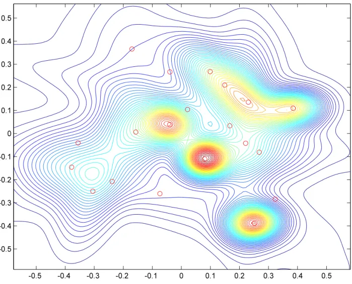
7 Random Landscapes 37
8 Banana Distribution 39
9 Free Energy Barriers 43
10 Conclusions 46
1
Introduction
Markov chain Monte Carlo (MCMC) methods are a remarkably robust way to sample from complex probability distributions. In this class of algorithms, the Metropolis-Hastings (MH) algorithm [1, 2] stands out as an important benchmark.
One of the appealing features of the original Metropolis algorithm is the simple physical picture which underlies the general method. Roughly speaking, the idea is that the thermal fluctuations of a particle moving in an energy landscape provides a conceptually elegant way to sample from a target distribution. Recall that for X, a continuous random variable with outcome x, we have a probability density π(x), and a proposal kernel q(x0|x). In the MH algorithm, a new value xnew is drawn from the distribution q and is then accepted with
probability:
a xnew|xold= min
1,q(x
old|xnew)
q(xnew|xold)
π(xnew)
π(xold)
. (1.1)
On the other hand, there are also well known drawbacks to MCMC methods. For exam-ple, though in many cases there is an expectation that sampling will converge to the correct posterior distribution, the actual speed at which this can occur is often unknown. Along these lines, it is possible for a sampler to remain trapped in a metastable equilibrium for a long period of time. A related concern is that once a sampler becomes trapped, a large free energy barrier can obstruct an accurate determination of the global structure of the distri-bution. Some of these issues can be overcome by sufficient tuning of the proposal kernel, or by comparing the performance of different samplers. It is therefore natural to ask whether further inspiration from physics can lead to new examples of samplers.
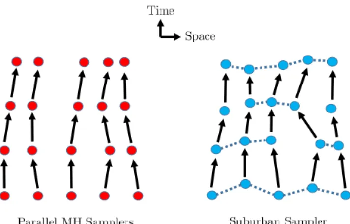
Now, although the physics of point particles underlies much of our modern understand-ing of natural phenomena, it has proven fruitful, especially in the context of high energy theoretical physics, to consider objects such as strings and more generally p-branes with finite extent in p spatial dimensions (a string being a case of a 1-brane). One of the main features of branes is that the number of spatial dimensions strongly affects how a localized perturbation propagates across its worldvolume. Viewing a brane as a collective of point particles that interact with one another (see figure 1), this suggests applications to questions in statistical inference [3].
Motivated by these physical considerations, our aim in this work will be to study gen-eralizations of the MH algorithm for such extended objects. For an ensemble of M parallel MH samplers of π(x), we can alternatively view this as a single particle sampling from M
variables x1, ..., xM with density:
Figure 1: Depiction of how parallel MH samplers (left) and a suburban sampler (right) evolve as a function of time. In the suburban sampler, nearest neighbors on a grid can have correlated inferences (depicted by dashed lines), leading to faster mixing rates. The absence of a dashed line in a given time step indicates a splitting of the extended object.
where the proposal kernel is simply:
qparallel(xnew1 , ..., x new
M |x
old 1 , ..., x
old
M ) =q(x
new 1 |x
old 1 )...q(x
new
M |x
old
M ). (1.3)
To realize an MCMC algorithm for an extended object, we shall keep the same target
π(x1, ..., xM), but we will now change the proposal kernel by interpreting the index σ on
xσ as specifying the location of a statistical agent in a network. Depending on the
connec-tivity of this network, an agent may interact with several neighboring agents (if each agent communicates with no neighbors, this is equivalent to parallel MH samplers). Schematically then, MCMC with an extended object involves modifying the proposal kernel to the form:
qextend(xnew1 , ..., x new
M |x
old 1 , ..., x
old
M ) = M Y
σ=1
qσ(xnewσ |Neighbors ofx
old
σ ). (1.4)
In the above, the connectivity of the extended object specifies its overall topology. For example, in the case of a string, i.e., a one-dimensional extended object, the neighbors of xi
arexi−1,xi, andxi+1. Figure 1 depicts the time evolution of parallel MH samplers compared
with the suburban sampler.
like the suburban algorithm, operate over identical copies of the target distribution; and those that operate over a parameterized family of related but not identical distributions. The former includes reference [5], which uses a population of samples to adaptively choose a proposal direction; reference [9], which use a population of samples to generate proposals that are invariant under affine transformations of the underlying space; and [10], which uses subsets of the sample populations to estimate parameters of an approximate distribution used to generate proposals in an elliptical slice sampler. The second category is exemplified by parallel tempering [7], in which parallel chains operate over a family of distributions parameterized by temperature where proposals include both local transitions and exchanges of state between pairs of chains. This category of methods uses distributions that mix better than the target distribution, but are similar enough to each other that exchanges will be accepted with reasonable probability. There are many MCMC variations in the literature that follow this general approach, including references [11–14].
Returning to the case of suburban samplers, there are potentially many consistent ways to connect together the inferences of statistical agents. From the perspective of physics, this amounts to a notion of distance/proximity between nearest neighbors in a brane. A physically well-motivated way to eliminate this arbitrary feature is to allow the notion of proximity itself tofluctuate. From the perspective of equation (1.4), we treat the placement of nearest neighbors as specifying a collection of random graphs, and by allowing possible fluctuations, various agents reach a collective inference differently. Indeed, from this perspective, it is also natural to allow the brane to split into or join up smaller constituent parts (see figure 1). In contrast to the case of a grid with a fixed topology, the physics of general splitting and joining is less tractable analytically (except in special limits where perturbation theory via a small expansion parameter is available).
Turning the discussion around, the general considerations presented here appear to have consequences for our understanding of quantum fields and strings. As noted in reference [3], one way to form approximate observables in a theory of quantum gravity is to consider inference of an ensemble of agents pooling their (approximate) local observations. From this perspective, the present paper can be viewed as a concrete implementation of this general proposal using the framework of Markov Chain Monte Carlo sampling. In particular, the appearance of a preferred role for an effective one-dimensional connectivity as predicted in [3] suggests a central role for such objects in any formulation of quantum gravity.
high density regions. Provided the connectivity with neighbors is sufficiently low, coupling these agents then has the potential to provide a more accurate global characterization of a target distribution. Conversely, connecting too many agents together may cause the entire collective to suffer from “groupthink” in the sense of [3], namely, once an initial erroneous inference is reached it can become difficult to correct. In the statistical mechanical inter-pretation of statistical inference developed in references [3, 15, 16], this can be viewed as the standard tradeoff in thermodynamics between minimizing the energy (i.e., obtaining an accurate inference) and maximizing entropy (i.e., exploring a broader class of configuration). In particular, we shall present some general arguments that the optimal connectivity for a network of agents on a grid arranged as a hypercubic lattice with some percolation (i.e., we allow for broken links) occurs at a critical effective dimension:
deff ∼1 (1.5)
where 2deff is the average number of neighbors.
To summarize: With too few friends one drifts into oblivion, but with too many friends one becomes a boring conformist.
To test these general theoretical considerations, we perform a number of numerical ex-periments for a variety of simple target distributions. One of the simple features of this class of proposal kernels is that there is a hyperparameter available (the average degree of connectivity) which allows us to smoothly interpolate from the case of an extended object to a collection of independent parallel MH samplers. Overall, we find that some level of connectivity leads to a generic improvement over parallel MH.
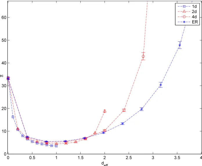
We address the extent to which the extended nature of a brane impacts its performance. Holding fixed the average effective dimension deff but varying the overall topology of the
extended object from a 1d, to 2d, to 4d grid, as well as an Erd¨os-Renyi ensemble of random graphs leads to comparable performance for the different samplers. In all of the cases we have encountered, the mixing rate is indeed fastest at a critical effective dimension as dictated by line (1.5). In some cases, however, the clumping effects of a higher dimensional grid are helpful, especially when there is a landscape of local maxima in the target distribution.
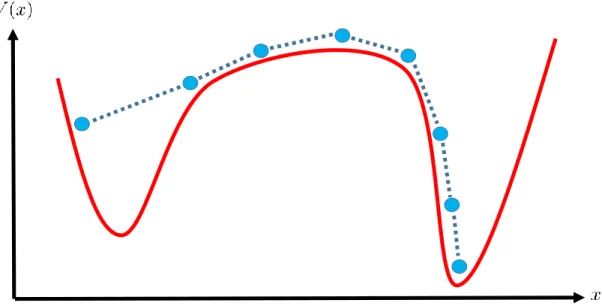
Figure 2: Depiction of how an extended object such as a string can overcome a free energy barrier.
study some controlled examples where we increase the free energy barrier between centers of a mixture model of two normal distributions, showing that as the barrier separation increases, the performance of parallel MH degrades more quickly than a deff ∼ 1 suburban sampler.
Section 10 contains our conclusions and potential directions for future work. In Appendix A we discuss in more detail the relative performance with slice sampling. For a condensed account of our results, we refer the interested reader to reference [17].
Finally, a standalone copy of the Java libraries for the suburban sampler, and its in-terface with the Dimple libraries is available at the publicly available GitLab repository
https://gitlab.com/suburban/suburban. We have also included a shortMatlabdemo for the suburban sampler.
2
Statistical Inference with Strings and Branes
To frame the results to follow, in this section we discuss both the physical motivation and applications connected with statistical inference with extended objects such as strings and branes.
theory, it is not entirely clear whether there is a completely well-defined notion of a local observable. Along these lines, it is fruitful to ask whether a collective of observers can agree in some approximate way on data measured by an ensemble. With this in mind, reference [3] proposed to study the observations of a collective of statistical agents pooling their resources to reach a final inference scheme. A concrete way to pose this question is to ask the sense in which the collective can accurately reconstruct a joint probability distribution such as:
π(x1, ..., xM) =π(x1)...π(xM), (2.1)
for M statistical agents. Following the general ideas presented in references [15, 16] for individual agents, statistical inference can be understood in terms of a statistical mechanics problem in which the relative entropy between an agents proposed probability distribution and the true distribution provides a notion of energy. This suggests a natural application to quantum gravity, where an individual observer may only have access to their individual “worldview” which is then improved by further samples of an actual data set.
Now, in quantum gravity there is a well-known issue with the use of point particles which stems from the fact that there is strictly speaking, no notion of a gauge invariant local observable. Rather, it is generally expected that some notion of locality must give way, and must also be accompanied by the appearance of spread out or extended objects. Along these lines, it is natural to ask whether an inference scheme adopted by an extended object can lead to different conclusions from those obtained by independent point particles.
This question was studied in reference [3], where general considerations led to the con-clusion that the standard conditions of quantum strings suggest a privileged role for one-dimensional objects. The main idea of [3] is that when statistical agents share data along a discretized worldvolume lattice, new inference schemes can be achieved which are unavailable to an individual agent. Additionally, there is a privileged role for 1 + 1 dimensional objects because in this case, the two-point function for a scalar field exhibits a late-time logarithmic divergence. This is milder than the power law divergence present for a free point particle, suggesting a more stable inference scheme relative to this case. Coupling this system to worldsheet gravity can also be understood at an abstract level as an additional layer of in-ference by a meta-agent, namely, where the connectivity between nearest neighbors can be rearranged.
there is also the question of the precise mechanism by which a collective actually “shares” information, namely how the pooling of resources in the entire collective actually takes place. One of the aims of the present paper will be to address these issues by showing how inference can actually be implemented for an extended object. Along these lines, we focus on the case of Markov Chain Monte Carlo sampling methods. The appearance of worldvolume gravity for the extended object will also be crudely characterized in terms of a statistical ensemble of random graphs, which act to define a time-dependent notion of locality for agents in the collective. In a certain sense this is a cruder notion of gravity than is present in the physical superstring, but it has the advantage of being discretized and fully non-perturbative. From this perspective, one should view the results of this paper as a concrete way to implement a non-perturbative formulation of strings and branes making observations in a target space.
The average degree of connectivity will provide us with a notion of an effective dimension. While this is admittedly less refined than the standard notions used in much of the high energy theory literature, it has the definite advantage of being completely well-defined so that we can implement and test it numerically. Indeed, even though it is crude, the remarkable fact that there is an effective dimension which appears to govern the main elements of the inference scheme is highly non-trivial and provides further evidence of the crucial role of effectively one-dimensional objects.
Finally, though we shall be implementing a Markov Chain Monte Carlo sampling algo-rithm the aim here is to better understand how the topology and dimension of a fluctuating lattice itself influences the overall speed and accuracy of an inference scheme. This is rather different from the standard approach in lattice quantum field theory where it is typically assumed that the lattice is fixed, and moreover, the structure of the target distribution π(x) is assumed to take a relatively simple canonical form. With these physical considerations in mind, we now turn to the implementation of MCMC with strings and branes.
3
MCMC with Strings and Branes
refer the interested reader to [20, 21], and references therein.
Suppose then, that we have a target distribution π(x). In an MCMC algorithm we produce a sequence of “timesteps”x(1), ..., x(t), ..., x(N) which can be viewed as the motion of
a point particle exploring a target space Ω. More formally, this sequence of points defines the “worldline” for a particle, and consequently a map from time to the target:
x: Worldline→Target with t7→x(t). (3.1) In the case of a string, we extend the notion of a “worldline” to a “worldsheet,” i.e., we have both a temporal and spatial extent with respective coordinates t and σ:
x: Worldsheet→Target with (t, σ)7→x(t, σ) (3.2) More generally, if we have an extended object with d spatial directions, we get a map from a “worldvolume” to the target:
x: Worldvolume→Target with (t, σ1, ..., σd)7→x(t, σ1, ..., σd). (3.3)
The cased= 0 and d= 1 respectively denote a point particle and string. To make the anal-ysis of these maps computationally tractable, we will have to discretize these worldvolumes. So, in addition to making finite timesteps, we will also have to work with a finite number of statistical agents spanning the spatial directions of the worldvolume.
Using this formulation, we shall extract some basic properties such as the correlation between samples as a function of time. In particular, we will see that the overall connectivity, i.e., the number of nearest neighbor interactions, strongly influences both spatial as well as temporal correlations. This spatial connectivity also affects the motion of the extended object on a fixed target. Compared with the case of independent point particles, this can allow an extended object to more easily explore global aspects of a target.
The rest of this section is organized as follows. First, we give a path integral formulation of MCMC for a point particle exploring a fixed target distribution. We then turn to the generalization for strings and branes, and introduce the notion of splitting and joining as well. After introducing the general formalism, we then turn to an analysis of how the average degree of connectivity for statistical agents in an ensemble impacts the resulting inference scheme.
3.1
Path Integral for Point Particles
In what follows, we denote the random variable as X with outcome x on a target space Ω with measure dx. We consider sampling from a probability density π(x). In accord with physical intuition, we view −logπ(x) as a potential energy, i.e., we write:
π(x) = exp(−V(x)). (3.4) In general, our aim is to discover the structure of π(x) by using some sampling algorithm to produce a sequence of values x(1), ..., x(N). A quantity of interest is the expected value of
π(x) with respect to a given probability distribution of paths. This helps in telling us the relative speed of convergence and the mixing rate. To study this, it is helpful to evaluate the expectation value of the quantity:
N Y
i=1
exp(−β(i)V(x(i))) (3.5)
with respect to a given path generated by our sampler. We can then differentiate with respect to theβ(i)’s to study the rate at which our sampler explores the target distribution. In more general terms, the reason to be interested in this expectation value comes from the statistical mechanical interpretation of statistical inference [3, 15, 16]: There is a natu-ral competition between staying in high likelihood regions (minimizing the potential), and exploring more of the distribution (maximizing entropy). The tradeoff between the two is neatly captured by the path integral formalism. Indeed, in the special case β(i) = 1 we have
an especially transparent interpretation: It tells us about a particle moving in a potential
V(x), and subject to a thermal background, as specified by the choice of probability mea-sure over possible paths. Indeed, we will view this probability meamea-sure as defining a “kinetic energy” in the sense that each time step, we apply a random kick to the trajectory of the particle, as dictated by its contact with the thermal reservoir.
Along these lines, if we have an MCMC sampler with transition probabilities T(x(i) →
x(i+1)), the expected value depends on:
Zpath(
β(i) ) = T(x(0) →x(1))e−β(1)V(x(1))×...×T(x(N−1) →x(N))e−β(N)V(x(N)) (3.6) Marginalizing over the intermediate values, we get:
Z =
Z
[dx]
N−1
Y
i=0
T(x(i) →x(i+1))e−β(i+1)V(x(i+1))
!
(3.7)
V(x) as a potential energy and −logT(x(i) →x(i+1)) as a kinetic energy. So, we shall write:
V(x) = −logπ(x) and K(x(i), x(i+1)) = −logT(x(i) →x(i+1)). (3.8)
We now observe that our expectation value has the form of a well-known object in physics: A path integral!1 For example, with allβ(i) = 1, we have:
Z(xbegin →xend) =
end
Z
begin
[dx] exp(−X
t
L(E)[x(t)]) (3.9)
where we have introduced the Euclidean signature Lagrangian:
L(E)[x(t)] =K+V. (3.10) Since we shall also be taking the number of timesteps to be very large, we make the Riemann sum approximation and introduce the rescaled Lagrangian density:
1
N
X
t
7→
Z
dt, N L(E)7→ L(E) (3.11)
so that we can write our process as:
Z(xbegin →xend) =
Z
[dx] exp
−
Z
dtL(E)[x(t)]
, (3.12)
where by abuse of notation, we use the same variable t to reference both the discretized timestep as well as its continuum counterpart.
A few comments are in order here. Readers familiar with the Lagrangian formulation of classical mechanics and quantum mechanics will note that we have introduced K +V
rather than K−V as our Lagrangian. In physical terms, this has important consequences, particularly in the interpretation of the time evolution of a saddle point solution (i.e., one that is solved by the Euler-Lagrange equations of motion). As an illustrative example, we see that for a quadratic potential, we do not obtain the familiar behavior of a harmonic oscillator with trajectory x(t)∼exp(iωt), but rather x(t)∼exp(−ωt). Formally, this amounts to the substitutiont 7→it, which is often referred to as a “Wick rotation” or passing to “Euclidean signature.” Physically, what it means is that rather than getting oscillatory behavior, we instead get a diffusion or spread to the location of the particle. For further discussion on Euclidean signature quantum field theory, i.e., statistical field theory, see for example [20,21]. To give further justification for this terminology, consider now the specific case of the
Metropolis-Hastings algorithm. In this case, we have a proposal kernel q(x0|x), and accep-tance probability:
a(x0|x) = min
1,q(x|x
0)
q(x0|x)
π(x0)
π(x)
. (3.13)
The total transmission probability is then given by a sum of two terms. One is given by
a(x0|x)q(x0|x), i.e., we accept the new sample. We also sometimes reject the sample, i.e., we keep the same value as before:
T(x→x0) = r×δ(x−x0) +a(x0|x)q(x0|x), (3.14) where δ(x−x0) is the Dirac delta function, and we have introduced an averaged rejection rate:
r ≡1−
Z
dx0 a(x0|x)q(x0|x). (3.15) The specific optimal value depends on the target distribution and the proposal kernel.2
For illustrative purposes, suppose that we work in the special limit where the acceptance rate is close to one, and that we have a Gaussian proposal kernel so that−logq x(t+1)|x(t)
∼
α x(t+1)−x(t)2
. In this case, the path integral takes a rather pleasing form which has a simple physical interpretation. We have:
High Acceptance: L(E)[x(t)] =K+V 'α x(t+1)−x(t)2+V(x(t)). (3.16) Where we interpret the finite difference between time steps as a time derivative:
Dtx≡x(t+1)−x(t). (3.17)
More generally, we can ask what happens for intermediate values of a. In general, this is a challenging question so we do not expect to have as simple a form for the Euclidean signature Lagrangian. Nevertheless, we shall see that much of the structure already found persists in this case as well. Along these lines, we shall attempt to approximate the mixture model T(x→x0) by a normal distribution qeff x(t+1)|x(t)
such that −logqeff x(t+1)|x(t)
∼
αeff x(t+1)−x(t)
2
. To this end, we match the first and second moments of the putative normal distribution with our net transition rate in the approximation that we can use the average acceptance rate a:
αeff =
1
a ×α. (3.18)
2For example, under the assumption that the limiting diffusion approximation is valid, the optimal
So in this more general case, we get the effective Lagrangian:
L(E)[x(t)]'αeff x(t+1)−x(t)
2
+V(x(t)) +..., (3.19) where here, the “...” denotes additional correction terms coming from:
Correction Term: −log(T(x→x0)/qeff x(t+1)|x(t)
). (3.20)
At a large number of samples, we expect that contributions given by higher order powers of time derivatives are suppressed by powers of 1/N, a point we discuss in more detail in subsection 3.3. Observe that as the acceptance rate decreasesαeff increases and the sampled
values all concentrate together.
Our plan in the following sections will be to assume the structure of a kinetic term with quadratic time derivatives, but a general potential. The overall strength of the kinetic term will depend on details such as the average acceptance rate. As we discuss in subsection 3.3, the correction terms to this general structure will, for a broad class of models, be suppressed by powers of 1/N.
3.2
Path Integral for Extended Objects
We now turn to the generalization of the above concepts for strings and branes, i.e., extended objects. To cover this more general class of possibilities, we first introduce M copies of the original distribution, and consider the related joint distribution:
π(x1, ..., xM) =π(x1)...π(xM). (3.21)
If we keep the proposal kernel unchanged, we can simply describe the evolution of M inde-pendent point particles exploring an enlarged target space:
Ωenlarged = ΩM = Ω×...×Ω
| {z }
M
. (3.22)
If we also view the individual statistical agents on the worldvolume as indistinguishable, we can also consider quotienting by the symmetric group on M letters, SM:
ΩSenlarged =XM/SM. (3.23)
We begin with some general definitions, and later specialize to more tractable cases. Along these lines, suppose we have a graph consisting of M nodes, and a corresponding undirected adjacency matrix A, which consists of ones on the diagonal, and just zeroes and ones off the diagonal. We also use σ as a general index holder for “spatial position” on a grid. We say that two nodesσ and σ0 are “neighbors” if Aσ,σ0 = 1. Denote by Nb(σ) the set
of neighbors for siteσ. Holding fixed the adjacency matrix A, we define the proposal kernel:
q(x1, ..., xM|y1, ..., yM, A)≡ M Y
σ=1
qσ(xσ|yNb(σ)), (3.24)
where qσ is some choice of proposal kernel for a single point particle.
We can therefore adopt two different perspectives on this procedure. On the one hand, we can view an extended object as propagating over the enlarged target. On the other hand, we can view this extended object as one collective moving on the original target space.
Indeed, much of the path integral formalism carries over unchanged. The only difference is that now, we must also keep track of the spatial extent of our object. So, we again introduce a potential energy V and a kinetic energy K:
V =−logπ and K =−logT, (3.25) and a Euclidean signature Lagrangian density:
L(E)[x(t, σA)] =K+V, (3.26)
where here,σA indexes locations on the extended object, and the subscriptAmakes implicit
reference to the adjacency on the graph. The transition probability is:
Z(xbegin →xend|A) =
Z
[dx] exp(−X
t X
σ
L(E)[x(t, σA)]), (3.27)
where now the measure factor [dx] involves a product over dx(σt). Since we shall also be
taking the number of time steps and agents to be large, we again make the Riemann sum approximation and introduce the rescaled Lagrangian density:
1
N
X
t
7→
Z
dt, 1 M
X
σ
7→
Z
dσA N M L(E) 7→ L(E) (3.28)
so that the expectation value has continuum description:
Z(xbegin →xend|A) =
Z
[dx] exp
−
Z
dtdσA L(E)[x(t, σA)]
in the obvious notation. Strictly speaking, the integral with measure dσA may fail to have
a smooth continuum limit (i.e., when M → ∞), so when it does not, no continuum ap-proximation is available and we should view this as merely a shorthand for the discretized answer.
3.2.1 Splitting and Joining
In the above discussion, we held fixed a particular choice of adjacency matrix. This choice is somewhat arbitrary, and physical considerations suggest a natural generalization where we sum over a statistical ensemble of choices. We shall loosely refer to this splitting and joining of connectivity as “incorporating gravity” into the dynamics of the extended object, because it can change the notion of which statistical agents are nearest neighbors.3 Along these lines, we
incorporate an ensemble A of possible adjacency matrices, with some prescribed probability to draw a given adjacency matrix. Since we evolve forward in discretized time steps, we can in principle have a sequence of such matrices A(1), ..., A(N), one for each timestep. For each draw of an adjacency matrix, the notion of nearest neighbor will change, which we denote by writing σA(t), that is, we make implicit reference to the connectivity of nearest neighbors.
Marginalizing over the choice of adjacency matrix, we get:
Z(xbegin →xend) =
Z
[dx][dA] exp(−X
t X
σ
L(E)[x(t, σA(t))]), (3.30)
where now the integral involves summing over multiple ensembles: the spatial and temporal values with measure factordx(σt), as well as the choice of a random matrix from the ensemble
with measure factor dA(t) (one such integral for each timestep). At a very general level,
one can view the adjacency matrix as adding additional auxiliary random variables to the process. So in this sense, it is simply part of the definition of the proposal kernel.
The topology of an extended object dictates a choice of statistical ensemble A. We illustrate this by giving some particular examples which we study in more detail later on. For a collection of M independent, but indistinguishable point particles, the ensemble of adjacency matrices is given by:
Aparticles=
SAS−1|A is the M ×M identity and S ∈SM . (3.31)
For an ensemble of strings, we have a notion of a nearest neighbor interaction, and so we
3It is not quite gravity in the worldvolume theory, because there is a priori no guarantee that our sum
also introduce a split / join probability pjoin:
Astring(pjoin) =
SAS−1 with:
S ∈SM,
Aσσ = 1,
Aσ,σ+1 =Aσ+1,σ = 1 with probability pjoin,
Aσσ0 = 0 otherwise
, (3.32)
where in the above, the index σ = M + 1 is identified with σ = 1. That is, we have a circulant matrix: Geometrically, we view 1, ..., M as arranged along a circle, with each link either on or off.
More generally, we can consider the case of a d-dimensional hypercubic lattice, i.e., an extended object indspatial dimensions. In this case, it is somewhat simpler to first introduce a m×...×m
| {z }
d
×m×...×m
| {z }
d
array with md = M, which we then repackage in terms of an
M ×M matrix. For a hypercubic lattice in d dimensions, we introduceAσ1,...,σd;σ10,....,σ0d, and
define the ensemble of arrays for a brane as:
Abrane(pjoin) =
SAS−1 with:
S ∈SM,
Aσ1,...,σd;σ1,...,σd = 1,
Aσ1,...,σk,...σd;σ1,...,σk+1,...,σd =
Aσ1,...,σk+1,...σd;σ1,...,σk,...,σd = 1 with probability pjoin,
Aσσ0 = 0 otherwise
. (3.33) We can repackage this as anM×M adjacency matrix by replacing the multi-indexσ1, ..., σd
by a single base m index:
i= 1 + (σ1−1) + (σ2−1)m+...+ (σd−1)md−1. (3.34)
Of course, in addition to these geometrically well-motivated choices, we can consider more general ensembles of adjacency matrices. For example, a configuration of random graphs with well studied properties is the Erd¨os-Renyi ensemble:
AER(pjoin) =
Aσσ = 1,
Aσσ0 =Aσ0σ = 1 with probability pjoin (σ 6=σ0)
. (3.35)
3.3
Dimensions and Correlations
To keep our discussion from becoming overly general, we shall initially specialize to the case of a hypercubic lattice of agents in d spatial dimensions arranged on a torus, and we denote a location on the grid by a d-component vector σ. We shall later relax these considerations to allow for the possibility of a fluctuating worldvolume.
For a fixed grid, each grid site has precisely 2d neighbors. In what follows, we shall find it convenient to introduce a set of d unit vectors:
e1 = (1,0, ...,0) (3.36)
e2 = (0,1, ...,0) (3.37)
... (3.38)
ed= (0,0, ...,1). (3.39)
We also specialize the form of the proposal kernel:
qσ(xσ(t+ 1)|Nb(xσ(t))) ∝exp
−α(xσ(t+ 1)−xσ(t))2
−
d P k=1
β(xσ(t+ 1)−xσ+ek(t)) 2
−
d P k=1
β(xσ(t+ 1)−xσ−ek(t)) 2
. (3.40)
This has a recognizable form, consisting of finite differences in both the time direction, and spatial directions of our brane. Along these lines, we introduce the notation:
Dtxσ =xσ(t+ 1)−xσ(t) (3.41)
D+kxσ =xσ+ek(t)−xσ(t) (3.42)
D−kxσ =xσ−ek(t)−xσ(t) (3.43)
so that the proposal kernel is given by:
qσ(xσ|Nb(xσ))∝exp −α(Dtxσ)2− d X
k=1
β(Dtxσ−D+kxσ)2− d X
k=1
β(Dtxσ −D−kxσ)2 !
.
(3.44) To proceed further, we observe that in a large lattice, the finite differences are well-approximated by derivatives of continuous functions. In this case, we can also write D+kxσ = −D−kxσ,
and we get:
qσ(xσ|Nb(xσ))∝exp −(α+ 2dβ) (Dtxσ)
2
−
d X
k=1
2β(D+kxσ)
2
!
. (3.45)
That is, we see the expected kinetic term for a (d+ 1)-dimensional quantum field theory in Euclidean signature.
So far, we have kept our analysis rather general. Now, we would also like to be able to take a canonical limit in which the strength of timelike jumps remains comparable in passing from the completely disconnected grid to the maximally connected grid. To this end, we now further specialize the choice of α as:
α= 2β−2dβ. (3.46)
The full proposal kernel now takes the form:
Y
σ
qσ(xσ|Nb(xσ))∝exp −2β X
σ
(Dtxσ)2+ d X
k=1
(D+kxσ)2 !!
. (3.47)
Now, just as in the case of the point particle path integral, we again see that the effective transition rate defines a kinetic energy term, with an effective strength dictated by the overall acceptance rate. The general form of this kinetic term is given by a form recognizable to physicists:4
L(E)[x(t, σ)] = 2βeff
X
σ
(Dtxσ)
2
+
d X
k=1
(D+kxσ)
2
!
+V +... (3.48)
whereβeff sets the effective tension of the brane, and the correction terms “...” indicate that
we are again working to quadratic order in the derivatives. So to summarize, we have arrived at a (d+ 1)-dimensional statistical field theory with kinetic term quadratic in derivatives and a general potential.
One of the things we would most like to understand is the extent to which an extended object with d spatial dimensions can explore the hills and valleys of V. We perform a perturbative analysis, at first viewing V as a small correction to the propagation of our extended object. Starting from some fixed position x∗, we can then consider the expansion 4As the astute reader will no doubt notice, the structure of the kinetic term we consider here is not the most
general one we could consider. More generally, we can introduce a vector of temporal and spatial derivatives
DKx, withK = 0,1, ..., dand introduce the kinetic term 12(DKx) Σ1
KL
(DLx), with Σ a positive definite
of V around this point:
V(x) =V(x∗) +V0(x∗)(x−x∗) +
V00(x∗)
2 (x−x∗)
2+..., (3.49)
and study the impact on the correlation of samples as a function of time. Each of the derivatives of V(x) reveals another characteristic feature length of V(x). These feature lengths are specified by the values of the moments for the distribution π(x). Alternatively, we can simply use the various derivatives of V(x) to extract this set:
`n ∼
1 |V(n)(x
∗)|1/n
, (3.50)
An infinite value for the feature length simply means there is no new feature length.
Let us refer to the set of finite characteristic length scales as {`i}. Now, there is a clear
sense in which we can also view each of these length scales as defining a unit of time on the brane, i.e., how fast we expect our sampler to explore such a feature length. Using our Lagrangian interpretation, these length scales are set by both `i and the strength of the
kinetic term:
τi ∼`i× p
β. (3.51)
We refer to “early” and “late” time behavior as specified by:
tearly τi tlate. (3.52)
Since space and time on the worldvolume are on a similar footing, this also defines a notion of “close” and “far” for agents on the grid. By abuse of terminology, we shall lump all of these notions together.
Now, in the limit where V = 0, there is a well-known behavior for correlation functions:
hx(t, σ)x(0,0)i ≡ 1 Z
Z
[dx] x(t, σ)x(0,0) exp(−X
t X
σ
L(E)[x(t, σA)]) (3.53)
which for (t, σ)∈Rd+1 is given by:5
hx(t, σ)x(0,0)i ∼ 1
s
t2+
d P i=1
(σi)
2
!d−1. (3.54)
There is thus a rather sharp change in the behavior of the extended object for d < 1 and
5One way to obtain this scaling relation is to observe that the Fourier transform of 1/k2ind+1 dimensions
d >1. For d = 1, we have a logarithm rather than a constant. So, for low enough values of
d, the extended object can wander around at late times, while for larger values, the overall spread in values is suppressed. The crossover between the two behaviors occurs at d = 1, i.e., the case of a string.
We would now like to understand the impact that adding a non-trivial potential energy will have on the structure of our correlation functions. In general, this is a challenging problem which has no closed form solution. We can, however, develop a picture for whether we expect these perturbations to impact the early and late time behavior of our sampler. Along these lines, we can introduce the notion of a “scaling dimension” for x(t, σ) and its derivatives. The basic idea is that just as we assign a notion of proximity in space and time to agents on a grid, we can also ask how rescaling all distances on the grid via:
N 7→λN M 7→λdM (3.55)
impacts the structure of our continuum theory Lagrangian. The key point is that provided
N andM have been taken sufficiently large, or alternatively we take λ sufficiently large, we do not expect there to be any impact on the physical interpretation.
Unpacking this statement naturally leads us to the notion of a scaling dimension for
x(t, σ) itself. Observe that rescaling the number of samples and number of agents in line (3.55) can be interpreted equivalently as holding fixed N and M, but rescaling t and σ:
(t, σ)7→(λt, λσ). (3.56) Now, for our kinetic term to remain invariant, we need to also rescale x(t, σ):
x(t, σ)7→λ−∆x(λt, λσ). (3.57) The exponent ∆ is often referred to as the “scaling dimension” for x obtained from “naive dimensional analysis” or NDA. It is “naive” in the sense that when the potential V 6= 0 and we have strong coupling, the notion of a scaling dimension may only emerge at sufficiently long distance scales. For additional discussion on scaling dimensions and their role in statis-tical field theory, we refer the interested reader to reference [23]. Note that because we are uniformly rescaling the spatial and temporal pieces of the grid, we get the same answer for the scaling dimension if we consider spatial derivatives along the grid. This assumption can also be relaxed in more general physical systems.
space or in time. Under a rescaling, we have:
Z
dtddσ (Dx)2 7→λ−2∆+d−1
Z
dtddσ (Dx)2. (3.58)
So, invariance of the action requires the exponent of λ to vanish, namely:
∆ = d−1
2 . (3.59)
Using this general sort of scaling analysis allows us to characterize possible effects of perturbations, and whether we expect them to drastically impact our inference scheme as we take N and M to be very large. As a first example, consider the effects of the “Correction Terms” in line (3.20). We expect that such contributions will take the form of higher powers inDx, possibly multiplied by powers ofx as well. The latter possibility mainly occurs when we have a proposal kernel which cannot be written as temporal and spatial derivatives on a grid, i.e., it plays less of a role in the considerations that follow.
So, with this mind, we can consider the behavior of a perturbation of the form (x)µ(Dx)ν.
Applying our NDA analysis prescription, we see that under a rescaling, the contribution such a term makes to the action is:
Z
dtddσ (x)µ(Dx)ν 7→λ−µ∆−ν(∆+1)+d+1
Z
dtddσ (Dx)2, (3.60)
However, using (3.59), we see that the overall exponent on the righthand side is:
−µ∆−ν(∆ + 1) +d+ 1 = (2−ν)(d+ 1)−µ(d−1)
2 . (3.61)
So in other words, terms of the form (Dx)ν forν > 2 die off as we takeN → ∞, i.e.,λ→ ∞.
Additionally, we see that whend≤1, we can in principle expect more general contributions of the form (x)µ(Dx)ν. The presence of such terms will not affect our general conclusions. For additional discussion on the interpretation of such contributions, see reference [3].
is small. The dividing line is set by whether the scaling dimension of the interaction term is smaller than d+ 1 (i.e., the number of spacetime directions we integrate over):
n(d−1)
2 ≤d+ 1. (3.62)
So, ford≤1, all higher order terms can impact the long distance behavior of the correlation functions, while for d >1, the most relevant term is bounded above by:
n ≤ 2d+ 2
d−1 . (3.63)
Now, in the context of MCMC, we would like for our extended object to be able to explore different contours of the energy landscape. This in turn means that if our brane has settled near a critical point, it is potentially sensitive to the higher order derivatives in V(x) as in equation (3.49). So, a priori, if V(x) possesses many non-trivial derivatives, taking d ≤ 1 provides a way to explore more of this landscape. More precisely, we can see that for sufficiently large d we cannot probe much of the global structure of the potential. For example, if we set n = 3, we see that d ≤ 5, i.e., six spacetime dimensions for the worldvolume.
On the other hand, there is also a strong argument to avoid takingd too small. The fact that the time dependence of the two-point function of a free Gaussian field goes as 1/td−1
means that there can be significant spread in the fluctuations of a low-dimensional object. This in turn means that such an object may execute a very long random walk before finding anything of interest (wandering in the desert).
So to summarize, for d sufficiently small (i.e., close to zero), we can expect to wander for a long time before finding anything of interest, while conversely, if d is bigger than one, “groupthink” takes over in the collective and it is impossible to move away from an initial inference.
Clearly, the value of d which is optimal will depend on the precise shape of the potential
V(x). Nevertheless, we can already see that there is potentially a significant advantage to correlating the behavior of nearest neighbor interactions.
3.3.1 Effective Dimension and Fluctuating Worldvolumes
so it can also potentially explore a landscape more efficiently than parallel point particles. To address this issue, we consider a fluctuating worldvolume, i.e., we take an ensemble of nearest neighbors which actually fluctuates as a function of time.
Since we are now dealing with a fluctuating number of nearest neighbors, we will need to modify our proposal kernel. We again introduce a set of finite differences, but now we specifically indicate the neighbor as n(σ):
Dtxσ =xσ(t+ 1)−xσ(t) (3.64)
Dn(σ)xσ =xn(σ)(t)−xσ(t), (3.65)
in the obvious notation. We now introduce a modified proposal kernel where the size of the time step ασ now depends on the number of neighbors:
qσ(xσ|Nb(xσ))∝exp
−ασ(Dtxσ)
2
−X
n(σ)
β Dtxσ−Dn(σ)xσ 2
(3.66)
= exp
−(ασ+ntotσ β) (Dtxσ)2− X
n(σ)
β Dn(σ)xσ 2
+X
n(σ)
2βDtxσDn(σ)xσ
,
(3.67) where ntot
σ denotes the total number of nearest neighbors to the site σ, and the parameter
ασ also depends on the total number of nearest neighbors:
ασ = 2β−ntotσ β. (3.68)
Due to the fluctuating topology, an analysis of the correlation functions is now more challenging. However, there are various approximation schemes available which provide a way to cover this case as well. One crude approximation we shall adopt is to consider the typical random graph chosen from a particular ensemble, and to then further assume that this is well-approximated by just the average degree of connectivity between an agent and its neighbors. For the ensembles introduced earlier, i.e., for a d-dimensional hypercubic lattice with some percolation, the average number of neighbors is:
Hypercubic Lattice: navg = 2d×pjoin (3.69)
while for the Erd¨os-Renyi ensemble, the average number of neighbors is:
Erd¨os-Renyi: navg = (M −1)×pjoin, (3.70)
For hypercubic lattices, we can also introduce the notion of an effective dimension:
deff =navg/2, (3.71)
a notion we shall also use (by abuse of terminology) for the Erd¨os-Renyi ensemble as well. With this in mind, we can reuse our previous analysis with a fixed connectivity, where we replace all occurrences of d by deff. In this case, there is no need to confine our discussion
to d being an integer. When we turn to our numerical experiments, we will indeed see that this approximation provides a reasonable leading order characterization of the dynamics of branes.
4
The Suburban Algorithm
Having motivated the study of MCMC with strings and branes, we now turn to some specific implementations of the suburban algorithm. For ease of exposition, we shall present the case of sampling a single continuous variable x. The generalization to a D-dimensional target (such asRD) is straightforward, though there are various ways to do this, i.e., we can either adopt MH within a Gibbs sampler, or a sampler with joint variables (i.e., we perform an update on all D dimensions simultaneously).6
Let us now turn to the structure of the suburban sampler. Recall that we are interested in a class of Metropolis-Hastings algorithms in which instead of directly sampling fromπ(x), we introduce multiple copies of the target and sample from the joint distribution:
π(x1, ..., xM) =π(x1)...π(xM). (4.1) 6To be more precise, the MH within Gibbs update for a target distribution p(x(1), ..., x(D)) with
sup-port on a D-dimensional space amounts to viewing this as a conditional probability p(x(1), ..., x(D)) =
p(x(i)|x(1), ..., x(bi), ..., x(D))p(x(1), ..., x(bi), ..., x(D)), where the notation
bi indicates that we omit this index.
The MH within Gibbs update is then given by sampling from just the univariate distribution:
Algorithm 1MH within Gibbs Introduce Γ ={1, ..., D} for i= 1 to D do
j ← draw from Γ
x(j)← sample from p(x(j)|x(1), ..., x(bj), ..., x(D)) using a 1D MH update.
return (x(1), ..., x(D))
Algorithm 2Suburban Sampler Randomly Initialize X(0) and A(0)
for t= 0 to N −1do
X(∗)← sample from q(X |X(t), A(t))
accept with probabilitya(X∗|X(t), A(t))
if accept = true then X(t+1) ← X(∗)
else
X(t+1) ← X(t)
A(t+1) ←draw from A
return X(1), ...,X(N)
We shall also refer to the proposal kernel as:
q(x1, ..., xM|y1, ..., yM, A) = M Y
σ=1
qσ(xσ|Nb(yσ)), (4.2)
where A is the adjacency matrix of the grid. To avoid overloading the notation, we shall write X(t) ≡ nx(t)
1 , ..., x (t)
M o
for the current state of the grid. In what follows, we write the MH acceptance probability as:
a Xnew|Xold, A
= min
1,q(X
old|Xnew, A)
q(Xnew|Xold, A)
π(Xnew)
π(Xold)
. (4.3)
We now introduce algorithm 2, the suburban algorithm.
An important feature of the suburban algorithm is that some of these steps can be parallelized whilst retaining detailed balance. For example we can pick a coloring of a graph and then perform an update for all nodes of a particular color whilst holding fixed the rest. There are of course many variations on the above algorithm. For example, in practice for each time step we shall perform a Gibbs update over ourM agents. For Gibbs sampling over the target, we then have a Gibbs update schedule with D×M steps, and for the joint sampler, it is over just M steps. We can also choose to not draw a new random graph
A(t) at each step, but rather only every T
draw steps. Other possibilities include stochastic
time evolution for A(t). To keep the analysis tractable, however, we will indeed stick to the
simplest possibility, performing an update on the graph topology at each sampling time step. Now, having collected a sequence of values X(1), ...,X(N), we can interpret this asN×M
performing an appropriate sum over the observables:
hxiπ ' 1
N M
X
σ,t
x(σt) (4.4)
(x− hxiπ)2π ' 1
N M −1
X
σ,t
x(σt)− hxiπ2
(4.5)
as well as higher order moments.
Let us discuss the reason we expect our sampler to converge to the correct posterior distribution. First of all, we note that although we are modifying the proposal kernel at each time step (i.e., by introducing a different adjacency matrixA∈ A), this modification is independent of the current state of the system. So, it cannot impact the eventual posterior distribution we obtain. Second, we observe that since we are just performing a specific kind of MH sampling routine for the distributionπ(x1, ..., xM), we expect to converge to the
correct posterior distribution. But, since the variablesx1, ..., xM are all independent, this is
tantamount to having also sampled multiple times from π(x). The caveat is that we need the sampler to actually wander around during its random walk;d ≤1 is typically necessary to prevent “groupthink.”
4.1
Implementation
We now turn to the implementation of the suburban algorithm we shall consider in subse-quent sections. To accommodate a flexible framework for prototyping, we have implemented the suburban algorithm in the probabilistic programming language Dimple [24]. This con-sists of a set of Java libraries with a Matlab wrapper. We have found this interface to be quite helpful in reaching the form of the algorithm presented in this work, as well as in performing different types of numerical experiments.
In the actual implementation, we have found it helpful to exclude some initial fraction of the samples, i.e., the process known as “burn-in.”We do this more for practical considerations connected with the diagnostics we perform than for any theoretical reason, since a sufficiently well-behaved MCMC sampler run for long enough will eventually converge anyway to the correct posterior distribution. In practice, we take a fairly large burn-in cut, discarding the first 10% of samples from a run, i.e., we only keep 90% of the samples. We always perform Gibbs sampling over theM agents. If we also perform Gibbs sampling over aD-dimensional target, we thus get a Gibbs schedule with D×M updates for each time step. For a joint sampler, the Gibbs schedule consists of just M updates.
outlined in section 3:
qσ(xσ|Nb(xσ))∝exp
−ασ(Dtxσ)2− X
n(σ)
β Dtxσ −Dn(σ)xσ 2
with ασ = 2β−ntotσ β,
(4.6) that is, we take an adaptive value for the parameter α specified by the number of nearest neighbors joined to xσ. As already mentioned in section 3, the main point is to ensure that
the overall strength of the kinetic term, i.e., the quadratic terms involving the temporal derivatives, does not dominate over the spatial derivatives.
In addition, we also implement the different choices of graph ensembles outline in subec-tion 3.2.1. We also include the opsubec-tion to not permute or “shuffle” the indexing of the agents. As a general rule of thumb, we find that switching off shuffling always leads to worse performance.
4.2
Hyperparameters
Let us now formalize the total list of hyperparameters for the suburban algorithm. The total number of timesteps is N, and the total number of agents is M. In addition to the total number of samples collected in a run, we have a choice of ensemble of random graphs, i.e., how we connect the agents together. There is a coarse parameter given by the overall topology of graphs on which we perform percolation. Additionally, we have introduced a class of ensembles where we permute the locations of agents on the grid. For a collective of parallel MH samplers, this has no effect (since there is no correlation between agents anyway), but for more general collectives, this can clearly have an impact. Indeed, we find that if we consider related ensembles in which shuffling is turned off, the performance suffers. We shall therefore confine our experiments to cases where shuffling is switched on. Finally, there is also a continuous parameter pjoin which dictates the probability of a given link in a graph
being active. This in turn translates to the effective worldvolume dimension experienced by an agent in the collective. Of course, the specific choice of ensemble of random graphs will also affect how much variance there is in the average degree of connectivity, though surprisingly, this seems to be a subleading effect in the tests we perform.
There are also many hyperparameters lurking in the proposal kernel. For the most part, we will focus on the case of equation (4.6), where there is just one tunable parameterβ. For a sampler in D dimensions, this naturally extends to a symmetric positive definite matrix
βIJ, in the obvious notation. The overall parameter β sets the “stiffness” or tension of the
kernel approaches the uniform distribution, and the effects of grid topology are expected to become weaker.
5
Overview of Numerical Experiments
Our emphasis up to this point has been on various theoretical aspects of the suburban algorithm, in particular, how to understand MCMC with extended objects. We now switch gears from theory to experiment, and ask how well such algorithms do in practice. Our plan in this section will be to give a list of the various metrics we shall use to gauge performance. We then discuss the class of samplers we shall study, and then give a brief overview of the target distributions we consider. In subsequent sections we turn to examples.
For simplicity, we focus on the specific case where the qσ of equation (1.4) are all normal
distributions in which the means and covariance matrix are dictated by the choice of nearest neighbors. In most cases, we consider MH within Gibbs sampling, though we also consider the case where joint variables are sampled, that is, pure MH. For target distributions we focus on low-dimensional examples of target distributions such as various mixture models of normal distributions, as well as the Rosenbrock “banana distribution,” which has most of its mass concentrated on a lower dimensional subspace.
Rather than perform error analysis within a single long MCMC run, we opt to take multiple independent trials of each MCMC run in which we vary the hyperparameters of the sampler such as the overall topology and average degree of connectivity of the sampler. Though this leads to more inefficient statistical estimators for our MCMC runs, it has the virtue of allowing us to easily compare the performance of different algorithms, i.e., as we vary the continuous and discrete hyperparameters of the suburban algorithm.
To gauge performance of the different runs, we focus on examples where we can ana-lytically compute various statistics such as the mean and covariance matrix of the target distribution, comparing with the value obtained from our MCMC samplers. We also cal-culate the expected number of samples on a tail to see whether the sampler spends the correct amount of time searching for “rare events.” We also collect the rejection rate and the integrated auto-correlation time (i.e., mixing rate) for the MCMC sampler.
5.1
Performance Metrics
The performance metrics we adopt can roughly be split into tests of how well the algo-rithm converges to the correct posterior distribution, i.e., external comparisons, as well as internal comparisons such as the mixing rate and rejection rate for the Markov chain.
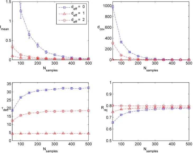
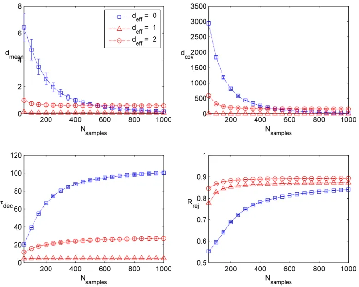
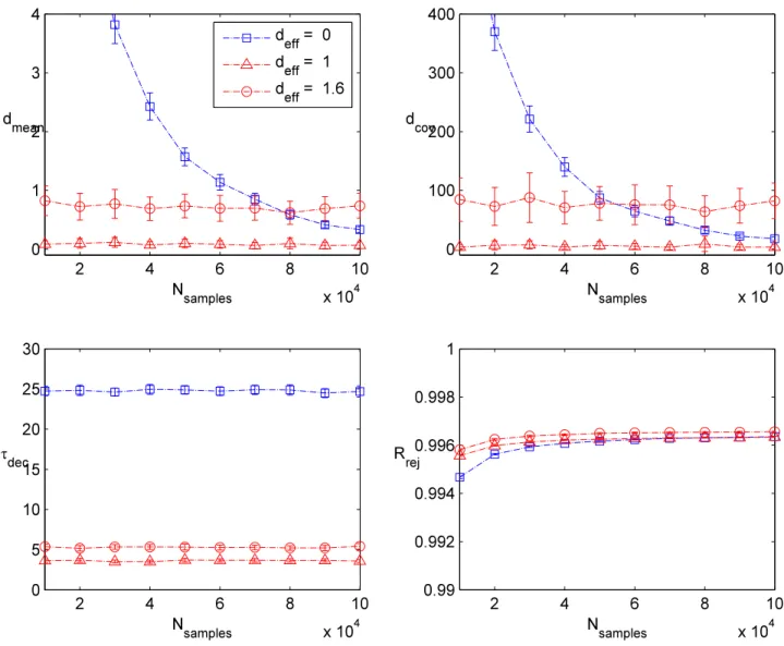
Let us now discuss each of these performance metrics in more detail. As a partial charac-terization of convergence to the correct posterior distribution, we focus on target distributions where we can calculate the various moments of the probability distribution analytically. In particular, for a D-dimensional target, we obtain a sample value for the mean and covari-ance matrix which we denote asµinf and Σinf, respectively, i.e., the inferred values. We then
compute the distance to the true mean and covariance using the metrics:
dmean ≡ kµinf−µtruek and dcov ≡
Tr(Σinf −Σtrue)·(Σinf−Σtrue)
T1/2
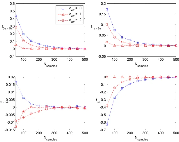
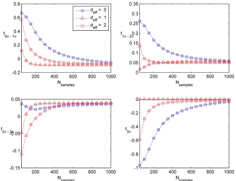
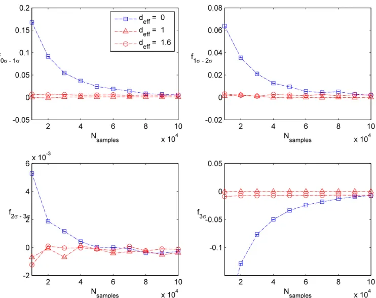
, (5.1) in the obvious notation. In addition to these simple tests, we also divide up the distribution into various regions of high and low probability mass, and verify that we obtain the appro-priate number of events in each of these regions. In practice, we always consider drawing a box of size LD centered at the origin such that there is a 68% chance of falling inside the box. We then also calculate the related 2σ and 3σ boxes (respectively 95% and 99.7%), and verify that a similar number of counts falls in the appropriate bin. In practice, we actually concentrate on the number of counts in the 0σ−1σ region, the 1σ−2σ region, the 2σ−3σ
region, and events which fall outside the 3σ region. For each such region, we compute the expected number of events with the observed number, and obtain a corresponding fraction:
fregion≡
Ninf−Ntrue
Ntotal
, (5.2)
where Ntotal denotes the total number of samples (after taking into account burn-in).
In addition to these external metrics, i.e., metrics based on comparison with the actual distribution, we also use diagnostics that are available from the MCMC runs. These are important in most actual applications of MCMC since we do not usually know the analytic form of the target distribution. Rather, we must depend on internal diagnostics such as the rejection rate, and the integrated auto-correlation time, i.e., the mixing rate. A typical rule of thumb is that for targets with no large free energy barriers, a rejection rate of somewhere between 50%−80% is acceptable (see e.g., [22]). Indeed, if the rejection rate is too low, then the sampler is wandering aimlessly, and if the rejection rate is too high, it is an indication that too little of the target is being explored. Let us also note, however, that in situations where there is a large free energy barrier (i.e., multiple high mass regions separated by large low mass regions), the rejection rate can turn out to be rather high. This is just a symptom of the fact that most proposals will land in a low mass region.
of the distribution. This observable provides a way of quantifying the correlation between samples drawn at different times from the MCMC run. This observable in particular has been argued to provide a preferred diagnostic for evaluating performance of an MCMC run (for a recent discussion, see e.g., [25]). Along these lines, we introduce:
V =−logπ(x1, ..., xM), (5.3)
and collect the values V(1), ..., V(N). We evaluate the covariance c(k) for−N < k < N,
c(k)≡
1 N N−k X t=1
V(t)−V
V(t+k)−V
for k≥0
1
N N+k X
t=1
V(t)−V
V(t−k)−V
for k <0
, (5.4)
and then extract the cross correlation bc(k):
b
c(k) =c(k)/c(0). (5.5) From this, we extract an estimate for the integrated auto-correlation time:
τdec ≡
X −N <k<N 1− k N
|bc(k)|= 1 + 2
N−1
X
k=1
1− k
N
|bc(k)| (5.6)
we also refer to this as the “decay time,”as it reflects how quickly the chain mixes. An important aspect of this analysis is that we explicitly include all samples here, i.e., we do not discard any samples from burn-in. When τdec is high, it means our samples are highly
correlated. To obtain a reliable estimate from an MCMC run, it is then necessary to either perform thinning, i.e. only take some sparse fraction of the original samples, or to run the sampler for even longer.
Now, for each of these observables, we could in principle extract standard errors using just a single run of the MCMC algorithm. We could also consider various sophisticated measures of convergence to the correct posterior distribution (see e.g., [26]). Since we have analytic control over the target distribution, we shall instead adopt a somewhat cruder approach to such error bar estimates: We simply repeat each experiment multiple times and collect both the means and standard errors on our observables. We do this primarily in order to not bias our analysis of errors which might otherwise depend on details of the algorithm. Along these lines, we perform T independent trials with random initialization for each agent on [−100,+100]D. We present all plots with a 3-sigma level standard error around the mean
value from these trials. In practice, we typically find acceptable error bars for T = 100 and
5.2
A Sampling of Samplers
Our primary interest is in the performance of the suburban sampler as we vary the different hyperparameters such as the grid topology; the split / join rate; and the tension β of the extended object. Now, in the special limit where we switch off all links between agents, we get a collection of M parallel MH samplers. We shall therefore interchangeably use the notationdef f = 0 and “parallel MH” samplers. Observe that this model also depends on the
hyperparameter β which controls the size of a proposed jump.
To gauge whether our performance is competitive with other simple examples of samplers, we also compare the performance of the suburban algorithm with slice sampling [27] within Gibbs. To make a more direct comparison with parallel MH, we also run M parallel slice samplers.
Even so, our goal is not to directly compare performance. There are a few general issues with doing so. In slice sampling, the algorithm typically queries the target distribution several times before recording a new sample value. In our comparison tests, we always keep fixed the total number of samples. So, whereas MH always evaluates the target distribution precisely twice on each loop (the new proposed value and the old value in the accept/reject step), the slice sampler will always make more evaluations of the target distribution. In practice, we find that the number of evaluations can be a factor of 5 ∼ 10 more when compared with MH. Since we have also not attempted to optimize the performance of a given algorithm, a direct comparison with either CPU time or “clock on the wall” time would also seem premature.
Even so, the crude comparisons we do perform point to the fact that for suburban sam-plers with stringlike connectivitydef f ∼1, the overall performance is comparable to parallel
slice samplers. For additional details on our implementation, and some example comparison runs, see Appendix A.
5.3
Example Targets
Let us now turn to the class of target space distributions we will use to test our suburban samplers. In general, there are of course many possible choices to make. Our examples are motivated primarily by the condition that we can easily track the effect of changes in the various hyperparameters.
The largest class of examples we consider are Gaussian mixture models in Ddimensions. These consist of k ≥ 1 components with a set of means µ(1), ..., µ(k) and covariance
matri-ces Σ(1), ...,Σ(k) so that the full target distribution is given by a weighted sum of normal
distributions:
πGMM(x) =
k X
l=1
Given sufficiently many experiments, we can tune the hyperparameters of an MCMC routine to optimize a given sampler. In our experiments, we will vary the number of mixtures, as well as the relative spacing between means and the alignment of the covariance matrices. Since our aim is to compare the performance of different samplers, we shall typically focus on models where we do not need to fine-tune the hyperparameters of the model to get reasonably accurate results.
As another class of examples, we also consider a case used in the study of optimization routines known as the two-dimensional Rosenbrock “banana function”:
πbanana(x, y|µ, α)∝exp(−(x−µ)2−α(y−x2)2). (5.8)
In the literature, it is common to take µ = 1 and α = 100, i.e., even though we have a two-dimensional target space, the high probability mass region is localized along the one-dimensional subspace y=x2. In such situations, we can expect Gibbs sampling routines to
fare poorly (a fact we verify), but MH samplers with joint variables still provide a way to accurately sample from such distributions.
As a final comment, to keep the timescale of all experiments short, we have also chosen to keep the total number of target space dimensions small, i.e., we focus onD= 2 andD= 10. We expect that at least for the Gibbs samplers, our conclusions continue to persist in higher dimensions. In the case of a joint sampler we can expect some decrease in performance at large dimension (a not uncommon issue in MCMC).
6
Effective Connectivity and Symmetric Mixtures
Perhaps the single most important feature of the suburban algorithm is that it correlates the inferences drawn by nearest neighbors on a grid. Quite strikingly, we find that the effective dimension rather than the overall topology of the grid plays the dominant role in the performance of the algorithm.
To illustrate this general point, we will primarily focus on a simple example in which we can isolate the effects of the different hyperparameters. We consider a class of target distribution examples which we refer to as “symmetric mixtures.”For a fixed choice of D
the number of target space dimensions, we introduce a mixture model consisting of 2D
components, with weights, means and covariance matrices:
p(±,l) = 1 2D, µ
(±,l)
i =±µ×δ l i, Σ
(±,l) =σ2×
ID×D, (6.1)
where i, j = 1, ..., D are indices running over the target, l = 1, ..., D indexes half of the components, and µ and σ are real numbers. Here, δl