4910.pdf

(1)

The gravitational field produced by extreme-mass-ratio

orbits on Schwarzschild spacetime

by Seth Hopper

A dissertation submitted to the faculty of the University of North Carolina at Chapel Hill in partial fulfillment of the requirements for the degree of Doctor of Philosophy in the Department of Physics and Astronomy.

Chapel Hill 2011

Approved by:

Charles R. Evans, Advisor

J. Christopher Clemens, Reader

Y. Jack Ng, Reader

Paul Anderson, Committee Member

(2)

c

(3)

Abstract

SETH HOPPER: The gravitational field produced by extreme-mass-ratio orbits on Schwarzschild spacetime.

(Under the direction of Charles R. Evans.)

A stellar-mass compact object orbiting a supermassive black hole will radiate energy and

angular momentum in the form of gravitational waves, causing it to spiral inward. Such an

extreme-mass-ratio inspiral (EMRI) is an important potential source for a direct gravity wave detection. It will require sufficiently accurate source modeling for such detections to

be made and analyzed. In this thesis I present original research that has furthered the

collective goal of accurate numerical EMRI simulations.

I begin by giving an overview of the extensive work that has been done in this field,

with an eye toward significant headway that has been made in the last decade. I then lay

the groundwork for my own work by reviewing the mathematical foundations for gravity

waves and black hole perturbation theory. Before attacking the subject of gravity waves

on a curved background, I examine the model problem of the scalar field that is induced

by an orbiting charge. This problem, while idealized, introduces many of the mathematical

and numerical techniques which are necessary to solve the perturbed Einstein equations.

At this point, with the foundation laid, I present new work on eccentric orbits of point masses about a Schwarzschild black hole. I show how the method of extended homogeneous

solutions is generalized to find the radiative part of the first-order metric perturbation in

Regge-Wheeler (RW) gauge using frequency domain techniques. Additionally, for the first

time we computed the local point-singular nature of the metric perturbation in RW gauge.

Due mostly to such gauge artifacts, RW gauge is not ideal of performing a local self-force

calculation. Thus, I then present work on transforming the metric perturbation to Lorenz

gauge. This will allow for the direct calculation of the self-force. I end this thesis by

(4)

Acknowledgments

My family has been exceptionally generous as I have worked toward my degree. In particu-lar, I’m grateful for all the kindness shown to me by my sister Marie and my brother-in-law Joseph, who allowed me to partake of their hospitality on countless occasions.

(5)

List of Figures

3.1 With the inclusion of time to our diagram, we must compressyandzinto one

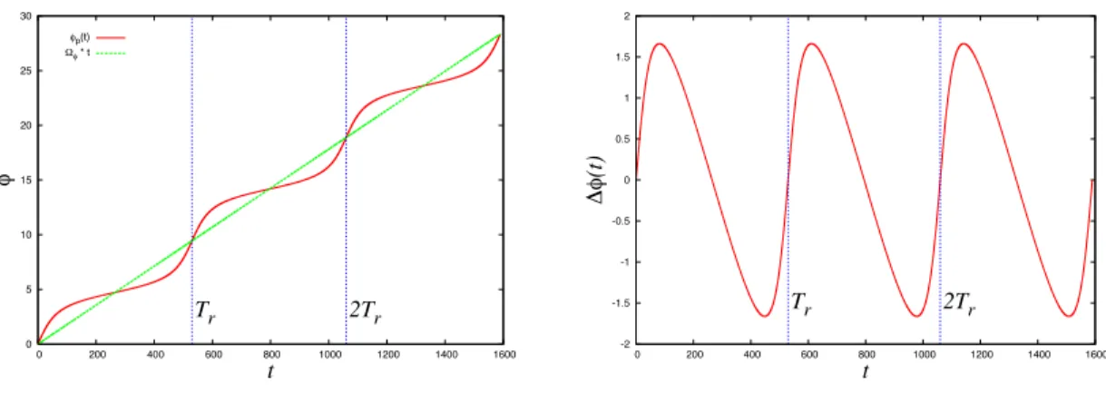
dimension. Hence, each sheet of time represents a three dimensional snapshot. 74 3.2 In red on the left we plot the azimuthal advance of a particle in eccentric

orbit around a Schwarzschild black hole. Its average advance Ωφtis plotted in

green. Subtracting off this average advance leaves the right panel. Note that this oscillation about the mean value of φhas a period of Tr, corresponding

to the radial motion of the particle. . . 87

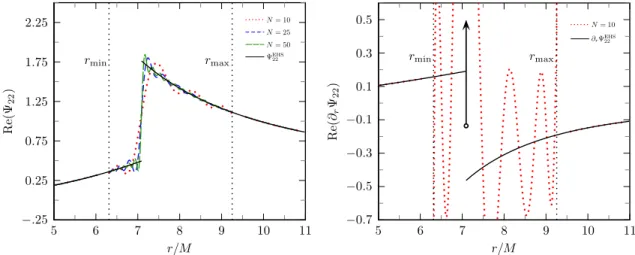
4.1 The standard FD approach to reconstructing the TD master function and its r derivative. The left panel shows Ψstd

22 and the right shows ∂rΨstd22 at

t= 51.78M for a particle orbiting with p= 7.50478 ande= 0.188917. This

figure is analogous to FIG. 1 of BOS [1]. Partial sums are computed with Eq. (4.3.3) and shown for different N. For contrast we plot the converged

solution from the new method with a solid curve (see FIG. 4.3). The arrow in the right panel gives a notional representation of the delta function singularity present in ∂rΨ22; the amplitude of this singular term is related to the jump in Ψ22 seen in the left panel. . . 106 4.2 An alternate view of the behavior presented in FIG. 4.1. A change in the

scale in the left panel emphasizes the Gibbs overshoots in Ψ22. On the right, a zoom-out of the vertical scale more clearly indicates the attempt of the Fourier synthesis to capture the delta function at rp(t). . . 106

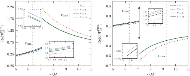
4.3 The EHS approach to reconstructing the TD master function and its radial derivative. As in FIG. 4.1, we give ΨEHS

22 and ∂rΨEHS22 at t = 51.78M for a particle orbiting with p = 7.50478 and e= 0.188917. Partial sums of ΨEHS

22 are computed from Eq. (4.3.5), with a range of−N ≤n≤N. The full ΨEHS

22 and itsr derivative result from N = 10, which gives agreement in the jumps

in ΨEHS

(9)

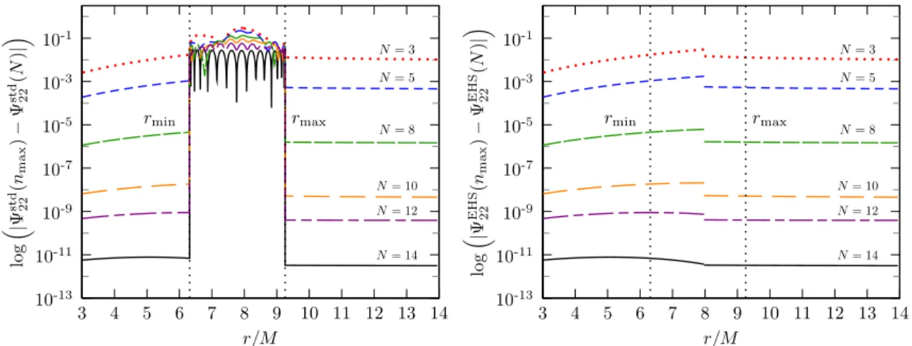
4.4 A plot of the convergence of the master function using the two methods. For a particle orbiting with p = 7.50478 and e = 0.188917 at t = 51.78M

we compute the master function Ψ22(nmax) by summing over modes ranging from ₋nmax ≤ n ≤ nmax for nmax = 15. We plot the log of the difference between Ψ22(nmax) and the partial sum Ψ22(N), for differentN < nmax. For the standard approach (left), we see exponential convergence in the homoge-neous region, but only algebraic convergence in the region of the source. The method of extended homogeneous solutions (right) yields exponentially con-verging results at all points outside and inside the region of the source. The method of extended homogeneous solutions gives exponential convergence for

∂rΨEHS`m as well. . . 118

4.5 The EHS approach to reconstructing the TD MP amplitudes. We consider a particle orbiting withp= 7.50478 and e= 0.188917 att= 80.62M. The left

plot shows the odd-parity MP amplitudes h21

r and h21t . The right shows the

even-parityh22

tt,h22rr,h22tr, andK22. Note that the amplitudesh22tt,h22rr, andh22tr

are singular along the particle’s worldline, as indicated by arrows in the plot on the right. The magnitude of these singularities are given in Eqs. (4.5.10), (4.5.13), (4.5.14). The remaining three MP amplitudes approach the particle location smoothly, and have only a finite jump at that point. . . 125

5.1 The Regge-Wheeler gauge metric perturbation amplitudeh21

t . As the particle

orbits between periapsis and apapsis, we examine the real and imaginary parts of this amplitude at a moment in time. In the left panel, note the (very slight) discontinuity at the location of the particle. In the right panel, note the lack of asymptotic flatness. . . 142 5.2 The Regge-Wheeler gauge metric perturbation amplitudeh21

r . As the particle

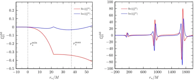
orbits between periapsis and apapsis, we examine the real and imaginary parts of this amplitude at a moment in time. In the left panel, note the discontinuity at the location of the particle. In the right panel, note the lack of asymptotic flatness. . . 143 5.3 The odd-parity RW → Lorenz gauge generator amplitudeξodd

21 . This differs from the Lorenz gauge metric amplitudeh21

2 (where the21are`, mindices on the amplitudeh2) by a factor of−2. Note that the fieldh212 grows asymptot-ically because it is a metric perturbation amplitude on the two-sphere, where an extra factor of r2 _{is present in spherical coordinates. Transforming to an} orthonormal frame would produce a field which falls off like 1/r, as radiation. 160

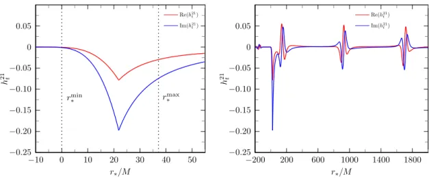
5.4 The Lorenz gauge metric perturbation amplitude h21

t . Note (comparing to

Fig. 5.1) the discontinuity at the location of the particle has vanished and the wave is not asymptotically flat. Note that the amplitudeh21

t is an off-diagonal

element of the metric perturbation, which introduces an extra factor of r in

(10)

5.5 The Lorenz gauge metric perturbation amplitude h21

r . Note (comparing to

Fig. 5.2) the discontinuity at the location of the particle has vanished and the wave is not asymptotically flat. Note that the amplitudeh21

r is an off-diagonal

element of the metric perturbation, which introduces an extra factor of r in

(11)

List of Tables

4.1 Total energy and angular momentum fluxes for eccentric orbits, compared with those from Fujita et al., published in [2]. . . 136 4.2 Energy and angular momentum fluxes for eccentric orbits, compared with

those from Fujita et al. [3]. Partial sums for all four orbits are truncated at

`max = 20 for both papers. Fujita et al. obtained their numbers from inte-grating the Teukolsky equation. We include this table to show the agreement of our horizon energy flux values. . . 136 4.3 Energy and angular momentum fluxes for an eccentric orbit withp= 8.75455,

e = 0.764124. Note that we have folded the negative m modes onto the

(12)

List of Abbreviations and Symbols

α, β, γ, . . . Spacetime coordinates indices running from 0 to 3 i, j, k, . . . Spatial coordinates indices running from 1 to 3

a, b, c, . . . Schwarzschild coordinates indices on the M2 _submanifold, _{_{t, r}_}

A, B, C, . . . Standard two-sphere coordinate indices on the _S2 _submanifold, _{_{θ, φ}_} g,Γ,R, . . . Sans-serif symbols indicate perturbed versions of their serifed counterparts µ Mass of the orbiting particle

M Mass of the central supermassive black hole

ηµν Minkowski metric

gµν Background metric

gab Schwarzschild metric on submanifold M2

ΩAB Metric on the unit two-sphere

gAB Metric on submanifold S2,gAB =r2ΩAB

Gµν Einstein tensor

Rαµβν Riemann tensor

Rµν Ricci tensor

R Ricci scalar

Γα

βγ Connection coefficients

∂µ or,µ Partial derivative

4_∇

µ,∇µ,or|µ Four-dimensional covariant derivative of the background manifold ∇a Two-dimensional covariant derivative on submanifold M2

DA Two-dimensional covariant derivative on submanifold S2

.

= Tensor components in a specific set of coordinates ∗

= Equality holds in a locally Lorentz frame

GW Gravity wave

EMRI Extreme-mass-ratio inspiral SMBH Supermassive black hole

FD Frequency domain

TD Time domain

RW Regge-Wheeler

EHS Extended homogeneous solutions EPS Extended particular solutions

MiSaTaQuWa Mino, Sasaki, Tanaka, Quinn and Wald BOS Barack, Ori, and Sago

(13)

Chapter 1 Introduction

1.1 The two-body problem in general relativity

The two-body problem stands as one of the classic unsolved problems of general relativity. The challenge is to take two gravitationally interacting objects with arbitrary initial

posi-tions and velocities (and potentially spins) and solve for their posiposi-tions and the gravitational

field at all future times. Given the complexity of the nonlinear, coupled Einstein equations,

it is impossible to solve such a problem, in general, through analytical approaches.

Re-searchers have therefore turned to numerical methods to provide solutions. Early work

involved post-Newtonian theory—work that goes back to Einstein at the dawn of general

relativity and Einstein, Infeld, and Hoffmann [4]. The first numerical relativity simulation

of a two-body system was made by Hahn and Lindquist, who attempted to collide two

non-rotating black holes head on [5] in 1964. Their code only ran for a brief time, and was not able to model the merger of the two holes. Still, it was the first step in what has

be-come an active and mature field. In recent years, interest in such simulations has increased

dramatically with the prospect of detecting gravitational waves.

1.1.1 Observational interest

Even beyond the inherent theoretical motivation for solving the two-body problem, there

exists a strong observational need to study this system. The detection of gravitational

(14)

bars) have been designed and built, interferometers have reached the most promising levels

of sensitivity. Gravity waves (GWs) produce slight time-dependent changes in the distances

between objects. Interferometers can detect these changes by measuring the time it takes

for photons to travel down to a mirror and back. Due to the extremely weak nature of

GWs, these detectors must be unprecedentedly sensitive. Detected GWs are anticipated to

cause fractional distance shifts of no more than one part in 1021_[6].

Detections will most likely be made by the Laser Interferometer Gravity-Wave

Obser-vatory LIGO [7]. LIGO is currently offline, as it is being upgraded with new components. When the upgrade is complete it will enter its third stage, dubbed Advanced LIGO.

Re-searchers are hoping the first gravity waves will be detected shortly after Advanced LIGO

goes online in 2014. If detected at LIGO’s two sites, and at the VIRGO [8] and GEO600

[9] detectors, a source of GW will be identified, localized and analyzed. These detections

will not happen, however, without sufficiently accurate theoretical models of GW sources.

Even the strongest astrophysical sources will produce GW signals that are buried deeply

in the noise of a detector’s data stream. Therefore, accurate theoretical models of a large

number of waveforms will be necessary in order to correlate with detector output. Processes

such as matched filtering can be used to extract a signal that has been masked by the various noise sources in a detector (e.g., seismic, thermal, and shot noise) [10].

In addition to their use in GW detection, accurate waveforms are also needed for source

parameter estimation. Black hole binaries produce complicated wave forms with as many

as fifteen parameters. For the case where the black holes have comparable mass, the field

of numerical relativity (NR) has been quite successful at modeling late-time waveforms. As

the mass-ratio becomes smaller NR calculations become progressively more challenging. At

this point, mass-ratios of 1:100 appear to be the outside limit of what is possible [11], and

even then the accuracy leaves much to be desired.

1.1.2 Extreme-mass-ratio inspirals

(15)

Hz ₋1 kHz, a range ideal for detection of binaries with comparable mass (_∼ 1₋10M) companions. Another likely astrophysical source of GWs are extreme-mass-ratio inspirals

(EMRIs) where solar-mass objects (∼1−10M) orbit supermassive black holes (SMBHs,

∼ 105₋₁₀7_M

). These sources are thought to exist in the centers of all major galaxies. For instance, the SMBH at the center of the Milky Way, Sagittarius A*, has a mass of

∼ 4.3_×106 _M

. M31 (the Andromeda Galaxy) has a SMBH of ∼108 M at its center. Small (µ . 100 M) compact objects orbiting such SMBH will radiate GWs at lower frequencies outside the LIGO passband.

In order to detect them, the European Space Agency (ESA) is planning a space based

interferometer detector. Until recently, this was to be a joint NASA-ESA mission named

the Laser Interferometer Space Antenna (LISA) [12]. NASA funding issues led to their

backing out [13]. At this point, ESA is reworking the mission to fit within a tighter budget.

It is not yet clear how the revised mission will change in specifications (or even name) from

the original joint plan. For the purposes of this discussion I will continue to call the mission

LISA and use the old specifications.

LISA will have a passband of ∼10−4 ₋₁₀−2 _{Hz, several orders of magnitude below}

LIGO. An EMRI is expected to stay in LISA’s passband for up to one million orbits as it spirals toward the SMBH and eventually plunges. The final stages of the inspiral will be

marked by an increase in frequency and amplitude until the small body plunges toward the

event horizon and a last burst of radiation is released. This increase in frequency and in

amplitude of the signal is called a chirp. The SMBH will then ring down exponentially as

it settles back to its usual stationary state.

As with ground based detectors, LISA’s detections will have to be pulled out of the noise

of its data stream. Therefore, tables of simulated waveforms will be needed for matched

filtering and parameter estimation. Given the types of different orbits that can exist and

the number of parameters, this is a formidable task. Astrophysical SMBHs are thought to be Kerr black holes, probably spinning at near maximal rates. In general, bound orbits in

the Kerr spacetime will be eccentric and out of the plane of the black hole’s rotation. The

(16)

distance to the source and its orientation relative to the detector. Finally, the small body

itself may be spinning, which can give rise to spin-orbit effects.

The previously mentioned method of general relativity simulations, numerical relativity

(NR), is not suited to the challenge of the EMRI problem. First there is a prohibitive

computational cost of such an approach. NR codes run on thousands of nodes, often for

months in order to compute 10’s of orbits. They work well for comparable mass systems

because of the similar length scales involved in the problem. The EMRI problem has two

distinct length scales: the background curvature associated with the SMBH, and the radius of the small body. The ratio of these two scales will be on the order of the mass-ratio,

which can be as small as 10−7_{. Even if one could resolve the different length scales, NR}

codes could not run with accuracy for the∼106_{orbits (as encountered with EMRIs) before}

plunge. It is for these reasons that researchers have turned to perturbative approaches.

1.2 Black hole perturbation theory

In black hole perturbation theory one takes a known solution to the Einstein equations

(typically that of a Schwarzschild or Kerr black hole) as a lowest order solution to the

gravitational field. Then, at lowest order in the equations of motion the small body, or

particle, moves on a geodesic of the background spacetime. This particle pulls up a

first-order perturbation to the gravitational field. Far away in the wave zone, it is evident

that this perturbation carries energy and angular momentum away from the system in the

form of gravitational waves. The energy loss comes at the expense of the particle’s orbit.

Locally, the inspiral that results can be viewed as the result of a “self-force.” In order to compute the self-force at the location of the particle, one must remove the singular part of

the particle’s field that does not contribute to radiation reaction. This procedure is called

“regularization.” One then seeks to find the way the orbit changes by solving the first-order

corrected equations of motion. This updated trajectory sources changes in the second-order

field, which in turn sources second-order corrections to the particle’s trajectory, and so on.

(17)

motion of the particle and gives the complete gravitational field. I go into the details of

first-order perturbation theory in detail in Chapter 2.

History

Black hole perturbation theory has a history going back to Regge and Wheeler [14] in 1957. They considered first-order perturbations to the Schwarzschild metric. In so doing,

they divided the metric perturbation into its even and odd-parity components and derived

their eponymous equation for the odd-parity perturbations. Their work was extended to

include a radial wave equation for the even-parity perturbations by Zerilli [15] in 1970.

Moncrief [16] re-derived both the Regge-Wheeler and Zerilli equations from a variational

principle without choosing a specific gauge. He also introduced gauge-invariant functions

of the metric perturbation amplitudes. Working with Cunningham and Price [17, 18], he

also introduced a more useful variable than Regge and Wheeler’s original odd-parity master function. Theirs is essentially the time integral of the Regge-Wheeler function and allows

for easier reconstruction of the odd-parity metric perturbation.

Important work was also done in 1975 in the field of quasi-normal modes by

Chan-drasekhar and Detweiler [19]. These modes describe how black holes ring down when they

are perturbed without a source. The least rapidly decaying such modes are of particular

interest for the time just after a particle plunges into a black hole.

Work on perturbations of the Kerr background was pioneered by Teukolsky [20] when

he presented the equation which now shares his name. The Teukolsky equation describes

the dynamics of the Weyl scalars (e.g., ψ4, ψ0), which are tetrad projections of the Weyl curvature tensor. There is a long history of results of computing solutions to the Teukolsky

equation for a small mass in order about a Kerr black hole. More difficult is determining

the metric from the computed curvature perturbations (see Chrzanowski [21], Cohen and

Kegeles [22, 23] (CCK), Stewart [24] and Wald [25]). The so-called CCK formalism is

powerful, yet only works for homogeneous solutions to the Teukolsky equation. Recent

work by Keidl, Wiseman, and Friedman [26] and others [27, 28] appears to have broken

(18)

the singular contribution to the Weyl scalars and then apply the CCK formalism to the

homogeneous solution which remains.

1.3 Flat space self-force

Before diving into self-force calculations in general relativity we start by discussing some simpler systems, which nonetheless contain many features in common with gravitational

self-force. I draw from many sources here, most notably Detweiler [29].

1.3.1 Newtonian self-force

Consider a simple two-body system described by Newtonian gravity. Let the first body have a massM and second body (or particle) of massµ, which we initially take to be vanishingly

small. At this lowest-order approximation the particle will travel in an ellipse with the

center of the large body at one focus, obeying Kepler’s laws. Let us consider the special

case of circular motion at radius r, where Kepler’s third law says the angular frequency of

the motion is

Ω2₌ M

r3. (1.3.1)

If we allow the particle to have a mass, then Kepler’s third law is [30]

Ω2 ₌ M

r3(1 +_µ/M)2. (1.3.2)

When µ _→ 0, the small body travels in a circle of radius r, but when we allow it to have

a mass, the two bodies orbit the common barycenter with a separationr(1 +µ/M). Now,

expanding in the small mass-ratio parameterµ/M, we find

Ω2 ₌ M

r3

1−2_Mµ +O

µ2

M2

. (1.3.3)

The first term is just the µ → 0 limit. The second term is a first-order correction, a

(19)

1.3.2 Radiation reaction in electromagnetism

Consider an accelerating, non-relativistic charge in flat space. It will radiate energy via

electromagnetic waves with a power calculable from Larmour’s formula (in Gaussian units)

[31]

P = 2e

2

3c3a

2_. _(1.3.4)

This can be used to derive the Abraham-Lorentz force

F= 2e

2

3c3a˙, (1.3.5)

from which one can compute the acceleration due to radiated energy loss. With careful

allowance for spurious solutions, this formula is useful for computing a particle’s change in

motion due to its own radiation reaction. However, it falls short in providing an explanation

for why the particle radiates. Indeed, it is at odds with the Lorentz force law which states

that acceleration is caused by an external electromagnetic field.

Consider, for concreteness, a non-relativistic electron in circular motion about a much more massive positive charge, which we take to be immovable. To an observer far away in

the wave zone, the electron will clearly pull up a 1/r radiation field which has a Poynting

flux that describes the energy lost by the system. On the other hand, an observer much

closer to the electron will measure the local electromagnetic field to be changing, but will

not be able to identify within it any hallmarks of radiation. Therefore, this second observer

will see the electron spiraling into the center, as predicted by Eq. (1.3.5), but will not be

able to describe this phenomenon as radiation reaction. Nor will he be able to explain the

inspiral as a result of some external field that sources the Lorentz force law.

Upon generalizing the Abraham-Lorentz force, Dirac [32] rectified this problem of

ob-server dependent descriptions of this system. Dirac generalized the system to include

rel-ativistic charges. He used a conservation of energy-momentum argument to show that the

(20)

Maxwell equations: F_{S ,ν}µν = 4πjµ_{. However, because of the relation between the retarded}

and advanced Green functions Gret(x, x0) = Gadv(x0, x), the field FSµν is invariant under

time-reversal. Therefore, it cannot be responsible for the radiation reaction. The

remain-der, which is responsible for the radiation reaction is

F_Rµν =F_retµν₋F_Sµν = 1

2 F

µν

ret −F

µν

adv

, (1.3.6)

where R stands for regular or remainder. The regular field is nonsingular everywhere and

a is homogeneous solution to the Maxwell equations. Furthermore, it produces the correct

acceleration when used with the Lorentz force law. Since Dirac’s initial work, others have

confirmed his results through different means. For a good summary see [33].

1.4 Curved space self-force

In curved space the problem of self-force becomes much more complicated. This is primarily

due to the fact that the retarded Green function no longer only has support on the past

light cone. Since radiation (both electromagnetic and gravitational) can scatter off of a

curved background (and even off itself in the case of gravity), the Green function also has support in the entire causally connected region inside the past light cone.

1.4.1 Electromagnetic self-force

Consider a particle with charge q in free fall in curved space. Here we are only concerned

with the electromagnetic (and not gravitational) radiation that is released as the charge accelerates. In their work on electromagnetic radiation reaction, Dewitt and Brehme [34]

separated the Green function into a direct part, which only has support on the light cone,

and a tail part, which has support inside the light cone. They follow Dirac’s conservation

approach and find that only the tail field contributes to radiation reaction. Their final result

is that the four-force on the charge due to radiation reaction is

(21)

This force is directly analogous to the Abraham-Lorentz force. It has great utility in that one

can compute the particle’s acceleration from it, but it is not consistent with the generalized

Lorentz force law Fµ ₌ _maµ ₌ _qFµν_u

ν. That is, the force in Eq. (1.4.1) does not result

from an external electromagnetic field. Indeed, an observer close to the particle would notice

its changing field, but being so close, would not be able to identify radiation. Therefore,

this near-observer would see no explanation for the particle’s motion as it deviates from

a background geodesic. Furthermore, the field Atail

µ is not a solution to the curved space

electromagnetic field equations.

Detweiler and Whiting [35] circumvented these conceptual obstacles by introducing a

different decomposition of the potential. They looked at the Green functions as follows. We

know the retarded Green function has support on and inside the past light cone while the

advanced Green function has support on and inside the future light cone. Define the singular

(S) Green function to have support in the spacelike area between the retarded and advanced

Green functions. Then, the regular (R) field will be the remainder AR

µ =Aretµ −ASµ. I will

not go into the details here, but the singular field is constructed specifically to remove the

Coulomb part of the particle’s field, which produces no force. The field FS

µν, constructed

from AS

µ, is a solution to the inhomogeneous curved space Maxwell equations. The

reg-ular remainder FR

µν, constructed from ARµ, is a homogeneous solution to those equations.

Furthermore, FR

µν appears to a local observer to be responsible for the entire self-force as

computed from the Lorentz force law.

1.4.2 Gravitational self-force

Here I consider the self-force on a small object moving in a curved spacetime. I sketch out

some of the most important results in this field. For a more thorough treatment see [36],

from which I draw heavily.

Historical perspective

A major milestone for the EMRI problem came in 1997 when Mino, Sasaki, and Tanaka [37]

(22)

on a curved background. The so-calledMiSaTaQuWa equations are first-order equations of

motion which (at least in theory) can be solved to give the deviation of a particle’s motion

off the background geodesic.

Mino et al. gave two derivations of the equations. The first was from a point particle

formulation. Point particles are useful, but their physical validity is questionable in certain

circumstances. For instance, a point particle pulls up a divergent 1/r local field which,

close enough to the particle, violates the fundamental assumption of perturbation theory

(that the particle’s field be small compared to the background). Their second derivation considered the more physical scenario of a small black hole moving on a curved background.

They used matched asymptotic expansions to show that the equations of motion of the two

systems were the same. This is an important discovery, as it justifies all the work that has

been done where the small black hole is modeled as a point particle, at least up to a certain

order in perturbation theory. Although a black hole is not a point particle, we are able to

treat it as such whenµ/M 1.

Detweiler and Whiting [35] provided a powerful reinterpretation of the self-force problem.

In the Detweiler-Whiting scheme, the particle’s retarded field is separated into regular R

and singular S parts. The former is a smooth field and a homogeneous solution to the

field equations. The latter is a solution to the inhomogeneous field equations, but gives no

contribution to the self-force. Therefore, the self-force can be found by substituting in the

regular field in for the retarded field in the equations of motion.

Mathematical formalism

Let a particle with massµmove in a spacetime dominated by a much larger body of massM.

For the large body alone, take a known solution to the Einstein equations, with the metric

gµν to be given. Black hole perturbation theory is an expansion around gµν with a small

expansion parameter taken to be µ/M. In our work we expand around the Schwarzschild

metric in Schwarzschild coordinates, but in principle it could be any solution. At lowest

(23)

stress-energy tensor, which serves as a source to the first-order field equations. We define

the difference between the true metricgµν and the background metricgµν to be the metric

perturbationpµν. To first-order, we find its solution by solving the field equations in Lorenz

gauge (see Chapter 2),

2p¯µν+ 2Rα βµ νp¯αβ =−16πTµν, (∇νp¯µν = 0). (1.4.2)

Here,2≡ ∇α∇αand we use an overbar to indicate a trace-reverse. Tµν is the stress-energy

tensor of a point particle. The retarded solution is

¯

pµν_ret(x) = 4µ

Z

γ0

Gµν_ret_αβ(x, z)uαuβdτ. (1.4.3)

HereGµν_ret_αβ(x, z) is the retarded Green function associated with Eq. (1.4.2) The parameter z represents the four spacetime coordinates being integrated over along the past geodesic.

The solution to these equations contains all the information about the first-order

gravi-tational field. At this point, the first-order field leads to a natural correction to the zeroth-order motion of the particle. By demanding the motion be geodesic in the perturbed

spacetime gµν we obtain the correction to the equations of motion

aµ₌₋1

2(gµν+uµuν) 2pretνα;β−pretαβ;ν

uα_uβ_. _(1.4.4)

This much appears straightforward enough, but a problem arises due to the local field of

the particle. The gravitational field of a point particle diverges like 1/ralong the particle’s

worldline, and therefore the force as calculated from the retarded metric perturbation is

divergent.

Yet, there clearly is a self-force. To the distant observer, the retarded metric

perturba-tion is plainly evident as radiaperturba-tion which falls off with the inverse of distance. This is seen

(24)

and yet there is no evidence for radiation. This paradox is once again resolved by the

sep-aration of pret

µν into singular (pSµν) and regular (pRµν) parts. The former is a solution to the

inhomogeneous equation 1.4.2, but provides no contribution to the self-force. The latter is

a smooth, homogeneous solution to Eq. (1.4.2), and fully responsible for the self-force. The

covariant derivative ofpR µν is

pR_µν_;_α=₋4µu(µRν)βαγ +Rµβνγuα

uβuγ+ptail_µνα, (1.4.5)

where

ptail_µνα =

Z τ−

−∞∇

α

Gretµνµ0_ν0z(τ), z(τ0)−1

2gµνG_retβ_βµ0_ν0

z(τ), z(τ0)

uµ0uν0dτ0. (1.4.6)

When we substitute inpR

µν forpretµν we obtain

aµ=₋1

2(gµν+uµuν)

2ptail_ναβ₋ptail_αβνuαuβ, (1.4.7)

which are the MiSaTaQuWa equations. They are first-order equations of motion which

give the particle’s acceleration off its background geodesic due to its own acceleration. An

important feature of these equations is that they are not generally covariant, but rather are derived specifically in Lorenz gauge. Indeed the self-force is not a gauge-invariant; its

change under a gauge transformation was computed by Barack and Ori [39]. One could even

choose a gauge where it vanishes at first-order [40]. This all serves to emphasize a crucial

point: in the end, we must calculate physically observable gauge-invariant quantities. Later

in this section we discuss this further.

The Detweiler-Whiting axiom and the conservative/dissipative split

The regular/singular split of the retarded field is very convenient, but not altogether obvious.

Detweiler and Whiting made their derivations from an axiomatic standpoint. Their axiom

(25)

This is analogous to the time-reversal symmetry of Dirac’s Coulomb field 1 2 F

µν

ret+F

µν

adv

,

which is clearly not responsible for radiation. However, the gravitational case is more subtle

because the gravitational self-force is responsible for more than just radiation reaction. The

gravitational self-force separates into two distinct pieces: conservative and dissipative.

The conservative piece is a consequence of the time-symmetric portion of the

gravita-tional field. It creates discrete shifts in the physical observables of the system. For example

(see Sec. 1.3.1), by adding a finite mass to the particle, one will naturally measure the

system to be that much more massive. Furthermore, the two objects will orbit around their common barycenter. Even beyond these Newtonian corrections, there will be changes to

the shape of the particle’s orbit, with contributions at every multipole order. The

symmet-ric, singular part is non-radiative and does not contribute to the dissipative piece of the

self-force. The conservative part of the self-force is

F_µcons = 1

2

F_µret+F_µadv₋F_µS. (1.4.8)

The dissipative piece of the self-force is the part responsible for radiation reaction, and

therefore only receives contributions from all modes`≥2. As mentioned, the singular part

of the perturbed metric is strictly conservative. Therefore, we can write the dissipative part

of the self-force as

F_µdiss= 1

2

F_µret₋F_µadv. (1.4.9)

Note that adding these two pieces together gives the regular field,

FR

µ =Fµcons+Fµdiss=Fµret−FµS. (1.4.10) Mode-sum-regularization

The separation of the gravitational field into regular and singular parts is quite useful in

numerical calculations. It provides two general paths forward toward computing the self-force.

(26)

the general idea behind mode-sum regularization, consider a scalar field ψ which is pulled

up by a particle with charge q orbiting a Schwarzschild black hole. (There is an exact

parallel to the gravitational case, just with more tedious equations) The scalar field will

satisfy the equation

2ψ(x) =q δ4(x, xp(τ)). (1.4.11)

Here 2 ≡ ∇α_∇

α, x, represents all four spacetime variables, and the particle travels on a

geodesic xp parametrized by its proper time τ. The field can be decomposed in spherical

harmonics, as shown in Chapter 3, which yields a radial wave equation for each`, m mode.

By imposing outgoing wave boundary conditions at spatial infinity, downgoing conditions

at the event horizon, and the correct internal jump conditions at the particle’s location, one

finds the retarded field at each mode, ψret

`m(x).

The idea, pioneered by Barack and Ori [41], is to then subtract off the singular part of

the self-force mode-by-mode. This subtraction is possible because, although the full field is

divergent, it is finite at each order. For a given`, taking the divergence ofψret

`m and summing

overm yields

∇αψret` =

X

m

∇αψret`m. (1.4.12)

Given this, we compute the self-force `-by-`from

F_α` =_∇αψ`ret−Aα(`+ 1/2)−Bα−

Cα

`+ 1/2 +· · · (1.4.13)

The full self-force Fα is then a convergent sum over the Fα`. The coefficients Aα, Bα, . . .

are called the regularization coefficients. They are independent of ` (though they depend

in general on the physical parameters of the problem) and are computed analytically.

Mode-sum regularization has been used successfully by numerous groups to compute self-forces due to scalar, electromagnetic, and gravitational fields from particles moving on

(27)

Effective sources

As an alternative to mode-sum regularization, there is the effective-source approach. This

was developed independently by Vega and Detweiler [42] and Barack and Golbourn [43].

Here, one computes pS

µν analytically, and then, the field is regularized by subtracting pSµν

frompret

µν and formingpRµν, which is formally smooth along the worldline (though in practice

will have a discontinuity at some order of differentiability). Having formedpR

µν, one can then

solve the first-order field equations, typically in the time-domain. Having already removed

the singular part, the self-force is trivial to compute at any stage in the integration. This

is a nice conceptual idea, though it does have several practical challenges. Foremost among

these is the analytic computation of pS

µν. The divergent, singular field can only be found

approximately, and even this is a tedious and lengthy task. An additional challenge arises

because far from the particle one wishes to have the retarded field, which contains relevant

information such as the gravitational waveform. Therefore, one typically uses a “window function” which transitions from the locally used regular field to the retarded field used

further away. Choosing an appropriate window function is a subtle task. For more details

see [44].

The gauge problem

As I have emphasized, the self-force is not a gauge-invariant quantity. The MiSaTaQuWa

equations are formulated in Lorenz gauge, and the regularization procedure is also Lorenz

gauge dependent. However, it is not always convenient to solve the field equation in Lorenz

gauge. As discussed in Chapter 2, significant simplification can be achieved on Schwarzschild

by choosing Regge-Wheeler gauge. And, until about seven years ago [45] nearly all work on

Schwarzschild was done in Regge-Wheeler gauge. The challenges entailed in transforming

from Regge-Wheeler to Lorenz gauge are covered in depth in Chapter 5.

One method of avoiding the gauge problem is to compute gauge-invariant quantities.

Physically measurable values such as the waveform are gauge-invariant. The mass and angu-lar momentum of an orbiting body are gauge-invariants. Of particuangu-lar interest is a quantity

(28)

was introduced for circular orbits on Schwarzschild and has since been generalized to

ec-centric orbits [47]. For a small body in orbit about a Schwarzschild black hole the local

observer will measure one value for the period of radial motion (local total proper time).

A distant observer will measure a different value for the period of the orbit. The ratio of

these two periods is Detweiler’s gauge-invariant quantity. Having such a quantity is useful

because one can compute the way it changes under a self-force correction in any gauge.

This is not only computationally convenient, but also good for checking results by taking

different routes to the same solution.

1.5 Original work: eccentric orbits on Schwarzschild

The previous sections of this introduction should give an overview of the current state of

research into the EMRI problem. Here I will give an overview of the contributions that I

have made to the field. My research has centered on eccentric orbits on a Schwarzschild

background. I will present some background on that specific problem and then summarize the new pieces I have added. For more detail, see Chapters 4 and 5.

1.5.1 Background

Generic eccentric orbits on Schwarzschild were first studied numerically by Tanaka, Shibata, Sasaki, Tagoshi, and Nakamura [48] and subsequently by Cutler, Kennefick, and Poisson

[49]. They used frequency domain (FD) methods to compute energy and angular momentum

fluxes from particles in a variety of orbits. FD codes have the benefit of converging very

quickly for mildly eccentric orbits, but as eccentricities grow they get less and less efficient.

Spurred largely by the work of Martel [50] and Haas [51], time domain (TD) codes have

gained great popularity in recent years. Additionally, until recently (see below) it was

impossible to accurately represent the gravitational field of a point particle in eccentric orbit

through FD calculations. This is due to the Gibbs phenomenon, which crops up because

(29)

Therefore, TD codes seemed necessary for local self-force calculations.

An additional change has taken place in recent years. Traditionally, most work on

Schwarzschild has been done in Regge-Wheeler (RW) gauge. RW gauge is attractive mainly

because it reduces the number of equations that must be solved for each mode from ten to

two. (This equation counting is a bit of a simplification, but the point is that RW gauge

makes it efficient to solve the Einstein equations.) The problem with RW gauge, as discussed

above, is that it is not ideal for self-force calculations. The MiSaTaQuWa equations, and

the mode-sum regularization scheme, are both formulated in Lorenz gauge.

There are two ways around the gauge problem. One is to solve the Einstein equations

directly in Lorenz gauge, as proposed by Barack and Lousto [45]. This adds its own

compli-cations, but does have the benefit that it gives the gravitational field in the desired gauge.

The other option is to solve the Einstein equations in RW gauge, as done usually, but then

transform the solution into Lorenz gauge, by solving the gauge transformation equations.

We have chosen the second option. We work in the FD and in RW gauge. Then, we

perform the gauge transformation to find the metric in Lorenz gauge.

1.5.2 Contributions of this thesis project

As mentioned, a major problem with FD work on eccentric orbits was the Gibbs

nomenon. In 2008, Barack, Ori and Sago [1] showed how to circumvent the Gibbs

phe-nomenon with the method of extended homogeneous solutions (EHS). They demonstrated

the method using the monopole term in a scalar field model problem. The standard Fourier

synthesis provides algebraic convergence for this field, and its derivative does not converge at all. The EHS method allows exponential convergence of both the field and its derivative,

including right up to the particle’s location.

In our 2010 paper [52], we showed how to extend the EHS method to all radiative

gravitational modes. Working in RW gauge, the source term has not only a delta function,

but also a derivative of a delta function term. We found that the EHS method was applicable

even with this more singular source term. From this we were able to reconstruct the metric

(30)

In finding the metric perturbation, we also examined the singular nature of RW gauge

in depth for the first time. We found the spherical harmonic amplitudes of the metric

perturbation to be discontinuous (C−1_{) in all cases and in some cases to contain} time-dependent delta function contributions. We were able to compute the time time-dependent

magnitudes of these jumps and the time dependent coefficients of the delta functions for

the first time.

Our work in the FD is noteworthy for two practical reasons. First, our results are far

more accurate (relative errors of ∼10−12_{) than those of standard TD codes (relative errors} of_∼10−7_{). Given the subtraction that takes place during the regularization procedure, one}

wishes to have as much accuracy as possible when computing the retarded field. Secondly,

our code is very fast, especially for low eccentricities. Simulations which could take days

on TD codes run in hours or minutes. Further, even relatively high eccentricities (e∼.9)

appear to give competitive runtimes to TD codes, especially when the benefit of the FD

accuracy is taken into account. Lastly, all this is based on single processor calculations.

Yet, our FD-based computations are easily ported to run on parallel computers.

Following this, we have begun work moving from RW to Lorenz gauge. Formally, the

gauge transformation is clear. The infinitesimal coordinate transformation is presented in standard relativity texts (e.g. [53]), and is only a few lines. However, the specifics are

far more subtle. Moving from RW to Lorenz gauge involves solving a set of coupled wave

equations for each harmonic mode. This is further complicated by the singular nature of the

source (which in this case is the divergence of the trace-reversed metric perturbation). The

problem was examined in some detail by Sago, Nakano, and Sasaki [54]. We have decided

to use their decomposition as a starting point and perform the transformation numerically

for the first time. Though we have not completed the entire task, there are a few details

worth noting here.

First, a FD solution to the gauge transformation equations is not a straightforward application of the EHS method. We have had to develop new techniques to treat the types

(31)

solutions. Both are covered in depth in Chapter 5. We have completed the odd-parity part

of the gauge transformation, and have seen that as expected the C−1 _{behavior in the} amplitudes is transformed to C0 _{behavior at} _r ₌ _r

p(t) in Lorenz gauge. Also, the RW

metric is non-asymptotically flat. In Lorenz gauge, we find that proper asymptotic flatness

is recovered.

The completion of the gauge transformation will leave us in an ideal situation for

com-puting the self-force. We will have a highly accurate computation of the retarded metric

perturbation in Lorenz gauge at all locations, including the location of the particle. This last part is key, as it is there where we must take the divergence and perform the regularization.

There are several paths forward from this point, as discussed in Chapter 6.

1.6 Thesis organization

This thesis is organized into five additional chapters. In Chapter 2, I provide an overview

of first-order black hole perturbation theory. I start with linearizing the Einstein equations around a Minkowski background and then generalize to a curved background. Finally, I

present the M2 _{× S}2 _{decomposition of Martel and Poisson [55], lay out the techniques}

of tensor spherical harmonics, and give the field equations for the metric perturbation

amplitudes in both Regge-Wheeler and Lorenz gauge.

Chapter 3 contains work on a scalar field model problem. The scalar field is an excellent

testing ground for work before jumping into gravity. Here I present the multipole

decom-position of a scalar field produced by a charged particle moving in flat space and show how

this is equivalent to an exact solution to that problem. Finally, I move to curved space and derive the field equations that must be solved for a scalar charge in eccentric orbit about a

Schwarzschild black hole.

Chapter 4 is taken from our first paper, Ref. [52]. It shows how we solved for the

radiative parts of a first-order metric perturbation due to a small mass in eccentric orbit

about a Schwarzschild black hole. In so doing we computed the metric perturbation to high

(32)

nature of the metric in Regge-Wheeler gauge.

Chapter 5 is a thorough discussion of subsequent results that will appear in a second

paper. It goes into the details of performing the first-order gauge transformation to take the

metric perturbation from Regge-Wheeler to Lorenz gauge. We give results there showing the

completed odd-parity transformation, as well as a significant component of the even-parity

part of the transformation.

Chapter 6 is a conclusion. I summarize the work presented in this thesis and give

(33)

Chapter 2 Mathematical preliminaries: gravitational

waves and black hole perturbation theory

The nonlinearity of general relativity makes finding exact solutions to the Einstein

equa-tions formidable and often impossible. Therefore, perturbative approaches are important for finding approximate solutions of all but the simplest physical systems. One approach

is post-Newtonian (PN) theory, wherein one expands the Einstein equations in powers of

v/c. PN has been very successful in checking the predictions of general relativity through

solar system [56] and binary pulsar experiments [57]. However, it fails in the strong field,

fast motion regime, which is where other perturbative methods must be employed. As an

alternative, one can consider a system wherein the mass-ratio µ/M of a two-body system

is very small. An expansion of the Einstein equations in this parameter yields equations

which are valid even as the small body is deep in the gravitational field of a black hole, and

traveling at speedsv.c.

Along with Chapter 3, this chapter sets the stage for my original research in Chapters 4

and 5. I start by reviewing how perturbing a flat metric leads to gravitational wave equations

in the context of linearized gravity. Using this as a model, I expand the Einstein equations on

a curved background and find wave equations for the first-order metric perturbation. This

expansion sets the theoretical foundation for finding the gravitational radiation emitted by

a small body in motion around a black hole. At this point I specialize to a Schwarzschild

spacetime, and use a decomposition introduced by Martel and Poisson [55] to separate

(34)

first-order Einstein equations in spherical harmonics. Further, I examine how those field

equations change under a gauge transformation. I end by giving the field equations for the

metric perturbation amplitudes in both Regge-Wheeler and Lorenz gauge, both of which

will be useful in subsequent chapters.

2.1 Linearized gravity

The presentation here follows closely that of [58, 53]. In the linearized theory of gravity, we

define our metric as

gµν =ηµν+pµν, |pµν| |ηµν|, (2.1.1)

and assume that space is asymptotically flat. All our work will be to first-order in pµν.

Using the Minkowski metric and its inverse to raise and lower indices, we define the inverse

of the metric perturbation as pµν _≡ _ηµα_ηνβ_p

αβ. A natural assumption is that the inverse

metric will vary from flat space by only a small amount, gµν = ηµν ₊_kµν_,_|_kµν_{| |}_ηµν_|_.

Then, we demand that gµαgαν =δµν, and find

δµν =gµαgαν = (ηµα+pµα) (ηαν +kαν) =δµν+kµν +pµν. (2.1.2)

(Note that the pµαkαν is dropped for being second-order.) So, evidently kµν =−pµν, and

the inverse metric is gµν =ηµν₋_pµν_.

In a coordinate basis, the connection coefficients are, to first-order

Γαβγ =

1

2ηαδ(pδγ,β+pδβ,γ−pβγ,δ). (2.1.3)

We form the linearized Riemann tensor in the standard way. After dropping terms quadratic

in the connection coefficients, this is

Rαµβν =

1

2(pαν,µβ+pµβ,να−pµν,αβ−pαβ,µν). (2.1.4)

(35)

we will drop any second-order terms. In order to transform geometric objects we need the

Jacobian matrix,

∂x0µ

∂xν =

∂xµ

∂xν +

∂Ξµ

∂xν =δ µ

ν + Ξµ,ν. (2.1.5)

The inverse transformation is also needed. We use the same logic that got us the inverse

metric perturbation. Demanding

∂xµ

∂x0α

∂xν =δ µ

ν (2.1.6)

and assuming the inverse transformation has a similar form to Eq. (2.1.5) we get

δµν =

∂xµ

∂x0α

∂xν = (δ µ

α+fµα) (δαν+ Ξα,ν). (2.1.7)

This defines fµν which is on the same order as Ξµ,ν. Expanding out the product, we find

fµ

ν =−Ξµ,ν, and so the inverse gauge transformation is

∂xµ

∂x0ν =δ µ

ν −Ξµ,ν. (2.1.8)

From this we can compute the transformation law for the metric (to first-order):

g0_µν =η_µν0 +p_µν0 = (δαµ−Ξα,µ)

δβν−Ξβ,ν

(ηαβ +pαβ) (2.1.9)

=ηµν+pµν−Ξν,µ−Ξµ,ν (2.1.10)

p0_µν =pµν−2Ξ(µ,ν). (2.1.11)

Note that this works because the Minkowski metric is gauge-invariant (ηµν = ηµν0 ). The

Riemann tensor changes under a gauge transformation as

R0_αµβν = (δγ

α−Ξγ,α) (δρµ−Ξρ,µ)

δδ

β−Ξδ,β

(δσ

(36)

Once again, we discard terms of higher than linear-order, so

R0_αµβν =Rαµβν−

δγ

αδρµδδβΞσ,ν+δγαδρµδσνΞδ,β

+δγαδδβδσνΞρ,µ+δρµδσνδδβΞγ,α

Rγρδσ (2.1.13)

=Rαµβν−

RαµβσΞσ,ν+RαµδνΞδ,β+RαρβνΞρ,µ+RγµβνΞγ,α

(2.1.14)

Up to now, we have considered a general, first-order gauge transformation for any form of the

Riemann tensor. Now, looking at Eq. (2.1.4) we see that this specific form of the Riemann tensor has no zeroth-order terms (because we are using flat space as our background).

Each term in it is linear in derivatives of the metric perturbation. Therefore, the terms

in Eq. (2.1.14) that involve products of Rαµβν and Ξµ,ν are all second-order. Hence, to

first-order the Riemann tensor (and therefore, each of its contractions) is gauge-invariant:

R0_αµβν=Rαµβν.

The Ricci tensor (which, as a contraction of the Riemann tensor, is also a

gauge-invariant) is

Rµν ≡gαβRαµβν =

1

2 pαν,µα+pµα,να−pµν,αα−pαα,µν

. (2.1.15)

The Ricci scalar is

R= 1

2(ηµν−pµν) pαν,µα+pµα,να−pµν,αα−pαα,µν

=pαµ,αµ−pµµ, αα . (2.1.16)

Definingp_≡pαα, we now form the Einstein tensor

Gµν ≡Rµν−

1

2gµνR (2.1.17)

= 1

2(pαν,µα+pαµ,να−pµν,αα−p,µν)−

1

2(ηµν+pµν)

pαβ,αβ−p,αα

. (2.1.18)

Then, the linearized field equations are (fromGµν = 8πTµν)

(37)

This simplifies if we express the metric perturbation in its trace-reversed form

¯

pµν ≡pµν−

1

2ηµνp ⇒ p=−p¯≡p¯αα. (2.1.20)

We use the overbar to represent a trace reversal in any tensor. Therefore Gµν = ¯Rµν and

pµν = ¯¯pµν. Plugging inpµν = ¯pµν−1₂ηµνp¯we have

¯

p_αν,µα₋1

2ηανp¯,µα+ ¯pαµ,να−

1

2ηαµp¯,να−p¯µν,αα

+1

2ηµνp¯,αα+ ¯p,µν −ηµν

¯

p_αβ,αβ₋1

2ηαβp¯,αβ+ ¯p,αα

= 16πTµν (2.1.21)

¯

p_αν,µα+ ¯p_αµ,να−p¯_µν,αα−ηµνp¯αβ,αβ = 16πTµν. (2.1.22)

From here it is standard [53] to choose the Lorenz gauge condition ¯pµν

,ν = 0. Three of the

four terms on the left side vanish and we get the linearized Einstein equations in Lorenz gauge,

2p¯_µν =₋16πTµν. (2.1.23)

It is instructive to show that one can always find a gauge that satisfies the Lorenz gauge

condition. First, the trace of the metric perturbation transform as p0µ

µ = pµµ−Ξµ,µ−

Ξµ,µ⇒ p0 =p−2Ξµ,µ.From this we can compute the transformation of the trace-reverse

of the metric perturbation,

¯

p0_µν =p0_µν−1₂ηµνp0 =pµν−2Ξ(µ,ν)− 1

2ηµν(p−2Ξα,α) = ¯pµν−2Ξ(µ,ν)+ηµνΞα,α (2.1.24)

Now, suppose that∂ν_p_¯

µν 6= 0. Perform a gauge transformation as described by Eq. (2.1.24),

and take the divergence of both sides:

∂νp¯0_µν =∂ν p¯µν−2Ξ(µ,ν)+ηµνΞα,α

. (2.1.25)

(38)

coordinates

0 = ¯p_µν,ν −Ξµ,νν−Ξν,µν+ηµνΞα,αν. (2.1.26)

The last two terms cancel because partial derivatives commute and we are left with an

inhomogeneous wave equation,

2Ξµ= ¯pµν,ν. (2.1.27)

We can reduce the full linear field equations (2.1.22) to the form of Eq. (2.1.23) by finding

any 4-vector Ξµ _{that satisfies Eq. (2.1.27). While this puts restrictions on the form of}

Ξµ_{, there is still residual gauge freedom because Eq. (2.1.27) is} _{inhomogeneous. Given a}

solution to an inhomogeneous differential equation, we can add any homogeneous solution

to it and get another inhomogeneous solution. To see this, assume the Lorenz gauge is

already satisfied. Then consider another linear-order gauge transformation

¯

p0_µν →p¯00_µν = ¯p_µν0 −2Ξ0(µ,ν)+ηµνΞ 0α

,α. (2.1.28)

Again, take the divergence of both sides and demand the left side vanish:

¯

p00_µν,ν = 0 = ¯p0_µν,ν −Ξ0µ,ν ν

−Ξ0ν,µ ν₊

ηµνΞ0α, αν

. (2.1.29)

Again the last two terms cancel. Now, recall that we’ve already demanded that the Lorenz

gauge be satisfied, so the first term on the right side vanishes also. Therefore, we are left with the following source-free wave equation that expresses the residual gauge freedom

2Ξ0

µ= 0.

Relation of the Lorenz gauge to the Bianchi identities

There are 10 algebraically independent Einstein field equations. Conservation of energy-momentum is expressed by the Bianchi identities,

∇ν_G

(39)

This is a set of four equations that limits the degrees of freedom inherent in the theory

down from 10 to 6. Consider now the linearized field equations in the Lorenz gauge (2.1.23).

Taking the divergence of both sides gives (note that in linearized gravity we take derivatives

with respect to the flat spacetime: ∇µ→∂µ)

∂ν2p¯_µν =2 p¯_µν,ν= 0 =₋16πTµν,ν = 0. (2.1.31)

This equation is satisfied identically. The left side is an expression of the gauge condition,

while the right is conservation of energy-momentum. Therefore, using the freedom of a

linear-order gauge transformation to remove four of the degrees of freedom from the full

equations of linear gravity is equivalent to removing the same four degrees of freedom by

imposing the Bianchi identities.

2.2 Perturbed Einstein equations in curved space

This section also draws heavily upon [53]. As an extension of the previous section, we now

consider small changes from a curved background. Consider a known, background solution

to the Einstein equationsgµν. A first-order perturbation to that metric,pµν yields

gµν =gµν+pµν |pµν| |gµν|. (2.2.1)

We denote covariant derivatives with respect to the background metric gµν with∇µ or |µ.

At first-order we raise and lower indices with the background metric. For the inverse metric

we find

δµν = (gµα+kµα) (gαν +pαν) =δµν+kµν+pµν +O(p2), (2.2.2)

and so as in flat space kµ

ν =−pµν, implying gµν =gµν−pµν.

Now, consider the transformation law for the connection coefficients,

Γ0α βγ =

∂xµ

∂x0β

∂xν

∂x0γ

∂x0α

∂xσΓ σ

µν−

∂xµ

∂x0β

∂xν

∂x0γ

∂2_x0α

(40)

The first term is the standard tensor transformation law, but the second term breaks the

tensor relation. However, notice that this term only depends on the coordinates (it is not

traced over any geometrical objects). So, if we take the difference between two covariant

derivatives, these terms cancel out and we find

S0αβγ =Γ0αβγ−Γ0αβγ =

∂xµ

∂x0β

∂xν

∂x0γ

∂x0α

∂xσ (Γ σ

µν −Γσµν) =

∂xµ

∂x0β

∂xν

∂x0γ

∂x0α

∂xσS σ

µν, (2.2.4)

where we use a sans-serif Γαβγ to represent the connection coefficient of the perturbed

spacetime Therefore,Sα

βγ obeys the tensor transformation law and is indeed a tensor.

We now compute Sα

βγ by using the standard connection coefficient expression to get

Sα βγ =

1

2gαµ(gµγ,β+gβµ,γ−gβγ,µ+pµγ,β+pβµ,γ−pβγ,µ)

−1₂gαµ(gµγ,β+gβµ,γ −gβγ,µ). (2.2.5)

Now, if we are in a locally Lorentz frame the background metricgµν =ηµν and its derivative

vanishes. Also, in that frame since connection terms (though not their derivatives) vanish

partial derivatives can be written as covariant derivatives (,µ=|µ). Therefore we have in the

locally Lorentz frame (we indicate an equality in a locally Lorentz frame with the symbol ∗

=)

Sα βγ

∗ = 1

2gαµ pµγ|β+pβµ|γ−pβγ|µ

. (2.2.6)

At this point, recognize that this is a tensor equation (note the importance of proving the

tensor nature of Sα

βγ), and thus it must be true in all frames, so

Sα βγ =

1

2gαµ pµγ|β+pβµ|γ−pβγ|µ

. (2.2.7)

(41)

perturbed Riemann tensor (Rα

βγδ) and the background Riemann tensor,

Rαβγδ−Rαβγδ=

h

∂γΓαβδ −∂δΓαβγ +ΓµβδΓαµγ−ΓµβγΓαµδ

i

−h∂γΓαβδ−∂δΓαβγ+ ΓµβδΓαµγ−ΓµβγΓαµδ

i

. (2.2.8)

Again consider a locally Lorentz frame where the background connection terms vanish. There, grouping terms we have

Rαβγδ−Rαβγδ

∗

=∂γ(Γαβδ −Γαβδ)−∂δ(Γαβγ −Γαβγ) +ΓµβδΓαµγ−ΓµβγΓαµδ. (2.2.9)

Because the background connections vanish, in this Lorentz frame we have Sα

βγ = Γαβγ.

Also, as before ,µ=|µ, and so

Rαβγδ−Rαβγδ

∗

=∇γSαβδ− ∇δSαβγ+SµβδSαµγ−SµβγSαµδ. (2.2.10)

Again, we notice that this is a tensor equation, and so it must be true in all frames,

Rαβγδ−Rαβγδ=Sαβδ|γ−Sαβγ|δ+SµβδSαµγ −SµβγSαµδ. (2.2.11)

Contracting over the first and third indices gives the difference in the Ricci tensors

Rβδ−Rβδ =Sαβδ|α−Sαβα|δ+SµβδSαµα−SµβαSαµδ. (2.2.12)

Direct calculations from Eqs. (2.2.7) and (2.2.12) give

Rβδ−Rβδ =∇α

₁

2gαµ pµδ|β+pβµ|δ−pβδ|µ

− ∇δ

₁

2gαµ pµα|β+pβµ|α−pβα|µ

+1

4gµνgαλ pνδ|β+pβν|δ−pβδ|ν

p_λα|µ+pµλ|α−pµα|λ

−1₄gµζgασ p_ζα|β+pβζ|α−pβα|ζ

p_σδ|µ+pµσ|δ−pµδ|σ

. (2.2.13)

4910.pdf

The gravitational field produced by extreme-mass-ratio

orbits on Schwarzschild spacetime

Abstract

Acknowledgments

Table of Contents

List of Figures

List of Tables

List of Abbreviations and Symbols

Chapter 1

Introduction

1.1

The two-body problem in general relativity

1.2

Black hole perturbation theory

1.3

Flat space self-force

1.4

Curved space self-force

1.5

Original work: eccentric orbits on Schwarzschild

1.6

Thesis organization

Chapter 2

Mathematical preliminaries: gravitational

waves and black hole perturbation theory

2.1

Linearized gravity

2.2

Perturbed Einstein equations in curved space