Liu_unc_0153D_18590.pdf

(1)

FLEXIBLE GRAPH-BASED LEARNING WITH APPLICATIONS TO GENETIC DATA ANALYSIS

Jianyu Liu

A dissertation submitted to the faculty of the University of North Carolina at Chapel Hill in partial fulfillment of the requirements for the degree of Doctor of Philosophy in the

Department of Statistics and Operations Research.

Chapel Hill 2019

Approved by: Yufeng Liu Shankar Bhamidi Wei Sun

(2)

(3)

ABSTRACT

JIANYU LIU: Flexible Graph-based Learning with Applications to Genetic Data Analysis (Under the direction of Yufeng Liu)

(4)

ACKNOWLEDGEMENTS

This dissertation would not have been completed without the great support of people who stood by me during my five years at UNC. I would like to thank all of them.

Firstly, I would like to express my sincere appreciation and gratitude to my advisor Professor Yufeng Liu for his continuous support of my Ph.D. research and career, for his patience, motivation, and immense knowledge. His guidance helped me throughout my research and writing of this thesis. He has always been supporting and encouraging me to make my own choices. I could not imagine having a better advisor and mentor for my Ph.D. study. I would also like to thank Professor Wei Sun for collaborating with me on the exciting projects and providing a lot of valuable suggestions on my thesis.

I would like to convey my sincere thanks to the rest of my thesis committee: Professor Shankar Bhamidi, Professor Quoc Tran-Dinh, and Professor Kai Zhang, for their time, support, guidance, and insightful comments on my dissertation.

(5)

TABLE OF CONTENTS

LIST OF TABLES . . . ix

LIST OF FIGURES . . . x

LIST OF ABBREVIATIONS AND SYMBOLS . . . xiii

1 Introduction . . . 1

1.1 Linear Discriminant Analysis and Its High Dimensional Extensions . . . 1

1.2 Graphical Models and Their Estimation . . . 3

1.2.1 The Gaussian Graphical Model and Its Extensions . . . 4

1.2.2 Count Data Graphical Models . . . 4

1.2.3 Directed Acyclic Graphs and Skeleton Estimation . . . 5

1.3 New Contributions and Outline . . . 6

2 Graph-based Sparse Linear Discriminant Analysis for High Dimensional Data . . . 9

2.1 Introduction . . . 9

2.2 Methodology . . . 11

2.2.1 Motivation and formulation of GSLDA . . . 11

2.2.2 Semi-supervised GSLDA . . . 16

2.3 Graph estimation and method implementation . . . 19

2.3.1 Graph estimation . . . 20

2.3.2 Parameter estimation and tuning parameter selection . . . 22

2.3.3 Pre-screening . . . 22

2.4 Theoretical properties . . . 23

2.4.1 Selection consistency . . . 23

(6)

2.5 Simulation study . . . 26

2.6 Real data analysis . . . 30

2.6.1 Arcene cancer data . . . 31

2.6.2 Semeion handwritten digits dataset . . . 32

2.7 Discussion . . . 33

3 Joint Skeleton Estimation of Multiple Directed Acyclic Graphs for Heterogeneous Population 34 3.1 Introduction . . . 34

3.2 Methodology . . . 35

3.2.1 Review of DAG estimation . . . 35

3.2.2 Joint estimation of multiple skeletons with hard labels . . . 37

3.2.3 Joint estimation of multiple skeletons with soft labels . . . 39

3.3 Computation of soft labels and tuning parameter selection . . . 40

3.3.1 Computation of soft labels . . . 40

3.3.2 Parameter tuning . . . 40

3.4 Theoretical properties . . . 41

3.5 Simulation studies . . . 42

3.5.1 Simulation settings . . . 43

3.5.2 Stage I: neighborhood selection . . . 45

3.5.3 Stage II: skeleton estimation . . . 46

3.6 Cancer genomic applications . . . 47

3.7 Conclusion . . . 52

4 Graphical Model Estimation for Single Cell RNA-seq Data . . . 54

4.1 Introduction . . . 54

4.2 Graphical Models based on scRNA-seq Data . . . 56

4.2.1 Existing count-data graphical models . . . 56

4.2.2 Dependent Poisson graphical models . . . 57

(7)

4.3 Implementation . . . 61

4.3.1 Estimation of the sample dependence . . . 61

4.3.2 Least squares approximation . . . 62

4.3.3 Tuning Parameter Selection . . . 62

4.4 Simulation Studies . . . 63

4.4.1 Simulation settings . . . 63

4.4.2 Non-zero-inflated data . . . 65

4.4.3 Zero-inflated data . . . 66

4.5 Real Data Analysis . . . 67

4.5.1 Exploratory data analysis . . . 68

4.5.2 Graph estimation . . . 71

4.6 Summary. . . 72

Appendix A Supplementary Materials for the GSLDA Method . . . 73

A.1 Some comments on the GSLDA method . . . 73

A.1.1 A graphical display of the discriminant vector decomposition . . . 73

A.1.2 Connection between GSLDA and existing methods . . . 73

A.2 Numerical results . . . 74

A.2.1 Graph estimation results . . . 74

A.2.2 Additional simulation results . . . 74

A.3 Proofs to the theoretical results . . . 77

A.3.1 Proof of Proposition 1 . . . 77

A.3.2 Proof of Theorem 1 . . . 77

Appendix B Supplementary Materials for the MPenPC Method . . . 84

B.1 Soft Label Demonstration . . . 84

(8)

B.2.1 Results of the ER Model Scenario . . . 84

B.2.2 Additional Settings . . . 84

B.2.3 Common Group Mean . . . 85

B.3 Assumptions and Proofs of the Theoretical Results . . . 86

B.3.1 Regularity Conditions . . . 86

B.3.2 Theorem 4 . . . 91

B.3.3 Theorem 1’ (Soft MPEN) . . . 95

B.3.4 Theorem 5 . . . 97

B.4 Datasets for the Real Data Analysis . . . 98

B.4.1 Cancer-Relevant Gene Sets . . . 98

B.4.2 PathwayCommons Dataset for Benchmark Graph . . . 98

Appendix C Supplementary Materials for Dependent Graphical Models . . . 100

C.1 Least Square Approximation . . . 100

C.1.1 Dependent Poisson Model . . . 100

C.1.2 Dependent Hurdle Model . . . 101

(9)

LIST OF TABLES

2.1 Performance comparisons of different classification methods for Example 1. . . 28

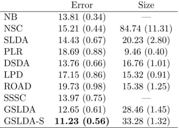
2.5 Comparison of GSLDA and other methods on the Arcene dataset. . . 31

2.6 Comparison of GSLDA and other methods on the Semeion dataset. . . 32

3.1 Performance of different methods at both stages for the BA-model examples (K= 4,p= 500,e= 1,π0 = 0.7 (High Overlapping) or 0.3 (Low Overlapping), andδ2 = 0.05). TPR =|G ∩ G|ˆ /|G|and FPR =|G \ G|ˆ /[(p2−p)/2− |G|], where G and ˆG denote the true and the estimated graphs respectively. The numbers outside and inside parentheses are averages and standard errors respectively based on 100 repetitions. . . 53

A.1 Graph estimation accuracy for all examples in the simulations. The graphs are estimated with labeled data (L) after centering, or with unlabeled data (U). The former estimation is compared with G, and the latter is compared with both G and ˜G. The results are averaged over 100 repetitions and the standard errors are provided in the parentheses. . . 74

B.1 Performance of different methods at both stages for the ER-model example (K = 4, p= 500, πE = 1/500, e= 1, δ2 = 0.05, π0 = 0.7 for high overlapping andπ0 = 0.3 for low overlapping). The numbers outside and inside parentheses are averages and standard errors respectively based on 100 repetitions. . . 87

B.2 Performance of different methods in the non-overlapping example (BA model, K = 4, p = 500, e= 1, δ2 = 0.05, π0 = 0). The numbers outside and inside parentheses are averages and standard errors respectively based on 100 repetitions. . . 88 B.3 Performance of different methods in the common group mean example (BA

model, K = 4, p = 500, e= 1, π0 = 0.7, δ2 = 0). The numbers outside and

(10)

LIST OF FIGURES

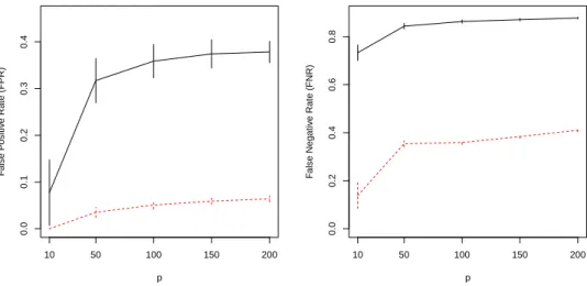
2.1 Performance evaluation of graph estimation for varying dimensions. The black solid lines are for graph estimation based on a labeled dataset of size 50; the red dashed lines are for graph estimation based on an unlabeled dataset of size 1000; vertical segments indicate the standard deviations of FPR or FNR of 100

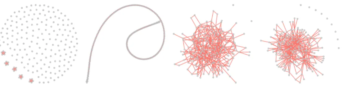
repetitions. . . 17 2.2 The graph structures used in the simulation study. From left to right: the

blockwise sparse model, the AR(3) model, the random sparse model, the scale-free model. The last two plots use one realization for demonstration, and the

graphs may vary among different realizations. . . 27

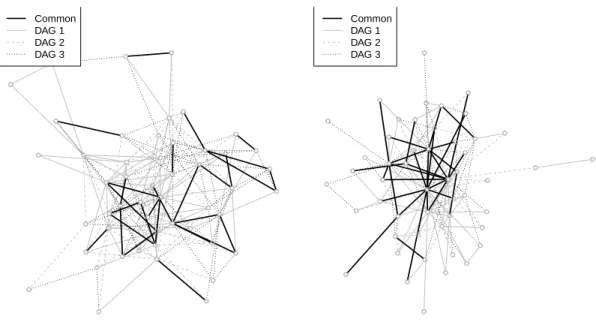
3.1 Examples of DAGs generated by the ER model (left) with πE = 0.02 and the

BA model (right) with e= 2. In both models, we set K= 3, p= 50, and π0 = 0.4.. . . 44 3.2 Neighborhood selection performance of different methods at Stage I in BA

scenario: K= 4,p= 500,e= 1,δ2 = 0.05,π0= 0.7 for (a) and 0.3 for (b). The x-axes andy-axes represent FPR and TPR respectively. The graph sparsity at the neighborhood selection stage varies for different tuning parameter λ. The

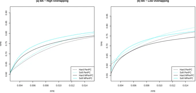
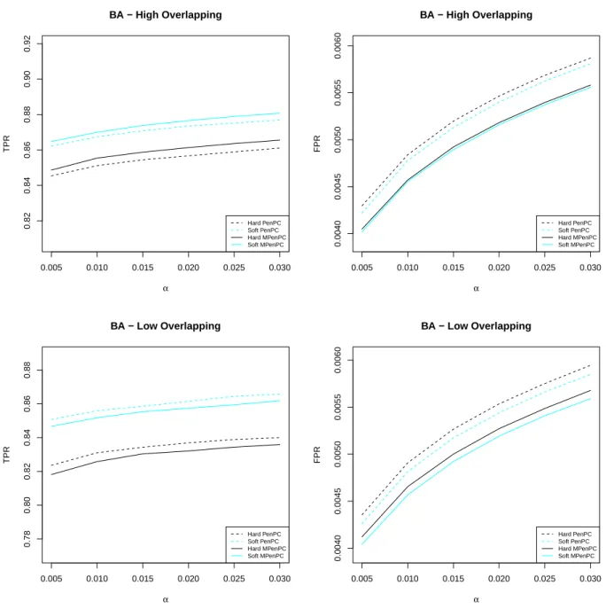
tuning parameterγ for MPenPC methods is preselected by EBIC. . . 46 3.3 Skeleton estimation performance of different methods at Stage II in BA

sce-nario. The high overlapping scenarios have π0 = 0.7, and the low overlapping scenarios have π0 = 0.3. The x-axes represent the significance level α of the PC-stable algorithm. They-axes represent TPR (the left panel) and FPR (the

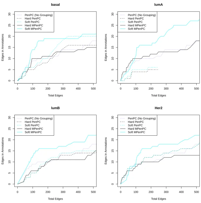
right panel) respectively. . . 48 3.4 Performance comparison of all methods at Stage I by cancer subtype. The

x-axes represent the total number of edges in estimated graphs corresponding to different λvalues; the y-axes represent the number of overlapping edges in

estimated graphs. . . 50 3.5 Performance comparison of all methods at Stage II by cancer subtype. The

x-axes represent the significance level α of the PC-stable algorithm. The y-axes represent the number of overlapping edges (left panel) and total number

of edges (right panel) in estimated skeletons. . . 51

4.1 Performance of different graph estimation methods under the non-zero-inflated setting (4.13). (a) Banded graph: µ1 =· · ·=µp = 0, c= 1/3; (b) Hub graph:

µ1 =· · ·=µp =−1,c = 0.5 ; (c) Random graph: µ1 =· · ·=µp = 1, c= 0.5.

The x-axes and y-axes represent FPR and TPR respectively. The sparsity of

(11)

4.2 Performance of different graph estimation methods under the zero-inflated set-ting (4.14). (a) Banded graph: µ1 =· · ·=µp = 0, c= 1, γ0 =−0.5, γ1 = 0.5; (b) Hub graph: µ1 =· · ·=µp =−1,c = 1,γ0 =−0.5, γ1 = 0.3; (c) Random

graph: µ1 = · · ·= µp = 2, c = 0.5, γ0 = 0, γ1 = 0.5. The x-axes andy-axes represent FPR and TPR respectively. The sparsity of estimated graphs by each

method varies by its specific tuning parameter. . . 67 4.3 Left: Histogram of the expression proportions of 1,960 genes in the Tirosh

and the Gierahn datasets. For example, more than 200 genes are expressed in only 30% – 35% of the cells in the Tirosh dataset. Right: The actual zero proportions versus the expected zero proportions for 1,960 genes under fitted

PLN model. . . 69 4.4 Left: Histogram of the sample correlation between cell pairs in the Tirosh and

the Gierahn datasets. Right: Histogram of the P-values of Pearson correlation

tests for all cell pairs. . . 70 4.5 Accuracy evaluation of graph estimation with real scRNA-seq datasets (left:

with dataset from Tirosh et al. (2016); right: with dataset from Gierahn et al. (2017)) . . 72

A.1 A 3-dimensional LDA example demonstrating how marginal differences of the three features (δ1, δ2, δ3) contribute to the predictive power of all features. Here ω23 =ω32 = 0. The terms around each node represent a decomposition of the corresponding coefficient. The gray scale of each term and the edge direction

together indicate the source of the marginal differences. . . 73 A.2 ROC Curve under the balanced setting for the four examples. The proportion

of Class-0 sample is 50%. The ROC curve is computed based on 100 repetitions.. . . 75 A.3 ROC Curve under the unbalanced setting for the four examples. In particular,

the proportion of Class-0 sample is 80%. The ROC curve is computed based

on 100 repetitions. . . 76

B.1 Accuracy of the estimated hard and soft labels for the toy example with vary-ing sample sizes. The y-axis denotes the Manhattan distance between the

estimated labels and true labels. Each boxplot is produced based on 100 repetitions. . . 84 B.2 Neighborhood selection performance of different methods at Stage I in the

ER-model example: K = 4, p = 500, πE = 1/500, δ2 = 0.05, π0 = 0.7 for (a) and π0 = 0.3 for (b). The x-axes and y-axes represent FPR and TPR respectively. The graph sparsity at the neighborhood selection stage varies for different choices of the tuning parameter λ. The tuning parameter γ for

(12)

B.3 Skeleton estimation performance of different methods at Stage II in the ER-model example. The high overlapping scenarios have π0 = 0.7, and the low overlapping scenarios have π0 = 0.3. The x-axes represent the significance levelα of the PC-stable algorithm. They-axes represent TPR (the left panel)

and FPR (the right panel) respectively. . . 86 B.4 Neighborhood selection performance of different methods at Stage I in the

non-overlapping example (BA model, K = 4, p = 500, e= 1, δ2 = 0.05, π0 = 0). Thex-axis andy-axis represent FPR and TPR respectively. The graph sparsity at the neighborhood selection stage varies with the tuning parameter λ. The

other tuning parameter γ for MPenPC methods is preselected by EBIC. . . 89 B.5 Skeleton estimation performance of different methods at Stage II in the

non-overlapping example (BA model, K = 4, p = 500, e= 1, δ2 = 0.05, π0 = 0). The x-axes represent the significance level α of the PC-stable algorithm. The

y-axes represent TPR (the left panel) and FPR (the right panel) respectively. . . 90 B.6 Neighborhood selection performance of different methods at Stage I in the

common group mean example (BA model, K = 4, p = 500, e = 1, π0 = 0.7, δ2 = 0). Thex-axis andy-axis represent FPR and TPR respectively. The graph sparsity at the neighborhood selection stage varies with the tuning parameter

λ. The other tuning parameterγ for MPenPC methods is preselected by EBIC. . . 91 B.7 Skeleton estimation performance of different methods at Stage II in the common

group mean example (BA model, K = 4, p = 500, e = 1, π0 = 0.7, δ2 = 0). The x-axes represent the significance level α of the PC-stable algorithm. The

y-axes represent TPR (the left panel) and FPR (the right panel) respectively. . . 92 B.8 The similarity, measured by lift(G₁,G₂) = (p2−p)/2· |G₁∩ G₂|/(|G₁| · |G₂|),

be-tween the LumA/LumB skeleton estimates and that bebe-tween the Basal/Lum skeleton estimates. Both the x-axes represent lift values of the LumA/LumB skeleton comparison. They-axes represent lift values of the Basal/LumA (left panel) and the Basal/LumB (right panel) skeleton comparisons. The simi-larities are computed based on skeleton estimation for each gene set by all methods. Different methods are in different colors, and the numbers annotate

(13)

LIST OF ABBREVIATIONS AND SYMBOLS

CIG DAG EBIC GSLDA LDA QDA scRNA-seq

G

D

Nj

Rn

Sn++

a−i

kak₂ kak∞

Ai,·

Aj

A−j

||A||∞

|||A|||∞

kAk_F

Conditional independence graph Directed acyclic graph

Extended Bayesian information criterion Graph-based linear discriminant analysis Linear discriminant analysis

Quadratic discriminant analysis Single-cell RNA-sequencing An undirected graph A directed graph

The neighborhood of predictor j in a graph Set of n-dimensional real valued vectors Set of n-dimensional positive definite matrices

The vector after removing the i-th element of the vectora

The `2 norm of the vector a

max{|a1|, . . . ,|an|}ifa is ann-dimensional vector

The i-th row vector of the matrixA

The j-th column vector of the matrix A

The matrix after removing the j-th column of the matrixA

max1≤i≤kPm_j₌₁|Aij|ifA is ak×m matrix

maxi,j|Aij|ifAis ak×mmatrix q

Pk i=1

Pm

(14)

CHAPTER 1

Introduction

Machine learning is a very important area for scientific research. Many machine learning techniques are shown to be very powerful for various applications. In this dissertation, we investigate several new based machine learning methods. In our first project, we propose a new graph-based classification technique. For our second and third projects, we study new approaches for graph estimation.

In this chapter, we provide some background knowledge and literature review on machine learning techniques. In Section 1.1, we introduce the linear discriminant analysis and its extensions in high dimensions. In Section 1.2, we briefly review graphical models, including Gaussian graphical models, count-data graphical models, and directed acyclic graphs (DAGs), and their estimation.

1.1 Linear Discriminant Analysis and Its High Dimensional Extensions

(15)

be-yond the Gaussian model. In particular, the same formulation can be obtained from the Fisher’s discriminant analysis problem (Fisher, 1936), the optimal scoring problem (Hastie et al., 1994), and linear regression (Hastie et al., 2009).

Despite the usefulness of LDA, it needs to be adapted when the dimension of features is high. For example, the form of standard LDA is only valid when the sample covariance matrix is invertible. Moreover, as the dimension grows, the errors in the sample covariance and group means accumulate and consequently LDA can become increasingly unstable (Fan and Fan, 2008; Shao et al., 2011). To address this problem, a number of LDA extensions have been proposed for high-dimensional scenarios.

Existing high-dimensional LDA methods in the literature can be roughly divided into two categories, plug-in approaches and direct approaches. A plug-in approach tackles high-dimensional problems by using regularized estimates for the within-class covariance matrix and group means. For example, the naive Bayes method, or the independence rule, treats the covariance matrix as diagonal. Bickel and Levina (2004) showed that it outperforms LDA with the Moore–Penrose pseudoinverse covariance matrix when the dimension grows faster than the sample size. To further reduce the instability of LDA, Tibshirani et al. (2002) additionally used shrunken estimates of group means. Fan and Fan (2008) showed that, even under the independence feature assumption, naive Bayes can be as bad as random guessing due to error accumulation in group means. They resolved this issue by reducing the dimension via feature screening. In contrast to these independence rules, Shao et al. (2011) assumed sparsity of the covariance matrix and the mean difference vector, and used thresholded estimates to construct a sparse LDA classifier. It was shown to be asymptotically optimal under certain conditions. All of these methods adopt the original formulation of LDA by calculating some improved estimates of the covariance matrix and group means. Thus, some strong assumptions on the covariance matrix and the group means need to be imposed for the resulting LDA rule.

(16)

which can be computed efficiently. Witten and Tibshirani (2011) also used Fisher’s discriminant analysis formulation for a generalK-class problem with a general regularization term. Clemmensen et al. (2011) proposed the optimal scoring formulation with the `1-penalty. Following the idea of minimizing the misclassification rates, Fan et al. (2012) proposed a method closely related to the method by Wu et al. (2009) and directly computed the misclassification rate of the classifier. Mai et al. (2012) took advantage of the regression formulation and estimated the discriminant vector of LDA by solving a Lasso-type problem, which was shown to have the same solution path as the method of Wu et al. (2009) and the method of Clemmensen et al. (2011) whenK = 2; see Mai and Zou (2013). Using a different idea for direct estimation, Cai and Liu (2011) formulated a linear programming problem to estimate β and showed that the error rate of the estimated classifier is close to the Bayes rule under certain conditions. Compared to plug-in approaches, these methods estimate LDA directly and the assumptions can be less stringent since only the sparsity of the discriminant vector of LDA is assumed (Cai and Liu, 2011).

Both plug-in and direct methods can work well for certain practical problems. However, these methods do not utilize the feature structure information when available. In practice, features are often correlated with some structure. Such structure can usually be represented by an undirected graphG. Connected features may work together and thus be effective or not effective simultaneously for classification. For instance, in the diagnosis of a disease using genetic information, genes are naturally grouped by their functions or gene pathways. Relevant genes tend to contribute or not contribute to the disease together. Moreover, when the population in consideration is Gaussian, the conditional independence graph, or the Gaussian graphical model, often represents a natural structure. By considering such structure information, we are likely to be able to construct a better classifier.

1.2 Graphical Models and Their Estimation

(17)

the graph. In the following subsections, we consider Gaussian graphical models and directed acyclic graphs respectively.

1.2.1 The Gaussian Graphical Model and Its Extensions

Among various graphical models, the Gaussian graphical model is possibly the most popular one for its simplicity and easy interpretation. For a multivariate Gaussian population, denoted as N(µ,Σ), the Gaussian graphical model is defined as the conditional independence graph, that is, each node represents a variable and two nodes are connected if they are conditionally dependent given the remaining nodes. It has been shown that the Gaussian graphical estimation is equivalent to finding the nonzero elements of the precision matrix, namely the inverse covariance matrix (Yuan and Lin, 2007). Moreover, in this scenario two variables are conditionally dependent if and only if one is in the partial regression model of the other with a nonzero coefficient.

Based on the above observations, many methods have been proposed for Gaussian graphical model estimation. For example, Meinshausen and B¨uhlmann (2006) proposed to estimate the graph by nodewise Lasso regression and showed the selection consistency. Similar works include Yuan (2010); Luo and Chen (2014a). Yuan and Lin (2007) and Friedman et al. (2008) proposed graphical Lasso that estimates the precision matrix via penalized likelihood. Cai et al. (2011) took advantage of the inversion relationship between the precision matrix and the covariance matrix and estimated a sparse precision matrix directly. Liu et al. (2009) and Liu et al. (2012) further generalized Gaussian graphical models for non-Gaussian data by non-paranormal transformation.

1.2.2 Count Data Graphical Models

Gaussian and non-paranormal graphical models often work well when the random variables or their continuous transformation are approximately Gaussian distributed. However, there are increasingly more scenarios in which this assumption is not true. For example, the Gaussian graphical model is typically not suitable for count data.

(18)

graphical models, of which the Poisson graphical model is a special case. But the model only allows negative dependence among the features. A number of approaches have been proposed to address this issue. Yang et al. (2013) proposed to remove such a restriction by modifying the base measure of the multivariate Poisson distribution. Allen et al. (2013) proposed a neighborhood selection approach that estimates the neighborhood of each node via penalized Poisson regression. See Inouye et al. (2017) for a comprehensive review. Recently, the Poisson-logNormal model has attracted a lot of attention for count-data graphical modeling. A variety of methods have been proposed for model estimation (Choi et al., 2017; Wu et al., 2018a; Sinclair and Hooker, 2017; Chiquet et al., 2018). However, none of them is feasible for high-dimensional modeling due to computational burdens.

Despite progresses on count-data graphical models, these existing models may not be appro-priate for some new data applications. In particular, the single cell RNA sequencing (scRNA-seq) techniques provide a way to study the gene expressions of each cell in a biological sample. However, there often exists substantial dependence among the cells and inflated zeros in the data. Thus new graphical models are needed to fit scRNA-seq data.

1.2.3 Directed Acyclic Graphs and Skeleton Estimation

There are many different types of graphical models. Besides undirected graphs, there is another type of graphs, namely the directed graph. One can tell from the name that they differ in the edge type: edges in a directed graph usually have directions. These directions sometimes may imply causal relationships, which makes directed graphs particularly suitable for causal inference.

(19)

possible to form a completed partially directed graph (CPDAG) using a set of deterministic rules (Pearl, 2009). We will focus on skeleton estimation in Chapter 3.

There are various approaches to estimate a DAG or its skeleton. A typical search-and-score approach searches for a skeleton that maximizes the regularized likelihood or the posterior prob-ability (Heckerman et al., 1995; Friedman and Koller, 2003). These methods can quickly become computationally infeasible for problems with thousands of variables. An alternative solution for skeleton estimation is constraint-based approaches, which are often more efficient computation-ally. Among these constraint-based methods, the PC algorithm (Spirtes et al., 2000; Kalisch and B¨uhlmann, 2007; Colombo and Maathuis, 2014), which is based on conditional independence tests, has been shown to be consistent in high dimension. There are also hybrid methods that combine the search-and-score and constraint-based approaches (Tsamardinos et al., 2006; Schmidt et al., 2007; Han et al., 2016). Nandy et al. (2015) showed that some hybrid methods with greedy search over the constrained DAG space are consistent under high dimensional settings. In a recent paper, Ha et al. (2016) proposed a two-stage skeleton estimation method called PenPC, which first estimates a conditional independence graph by neighborhood selection, and then estimates the skeleton by a modified PC algorithm.

In genetic study, the biological samples are often collected from individuals of multiple popula-tions. Each population can have a unique DAG structure while these DAGs may have a significant overlap. Since the population labels are often unknown, typical approaches for DAG (skeleton) estimation are to cluster or classify the samples into several groups and estimate a common DAG for all populations or a unique DAG for each population. However, these approaches either neglect the differences or do not take advantage of the similarities among the DAGs.

1.3 New Contributions and Outline

(20)

• In Chapter 2, we introduce a new high-dimensional LDA technique, namely graph-based sparse LDA (GSLDA), that utilizes the graph structure among the features. In particular, we use the regularized regression formulation for penalized LDA techniques, and propose to impose a structure-based sparse penalty on the discriminant vector β. The graph structure can be either given or estimated from the training data. Moreover, we explore the relationship between the within-class feature structure and the overall feature structure. Based on this relationship, we further propose a variant of our proposed GSLDA to utilize unlabeled data effectively, which can be abundant in the semi-supervised learning setting. With the new regularization, we can obtain a sparse estimate of β and more accurate and interpretable classifiers than many existing methods. Both the selection consistency ofβestimation and the convergence rate of the classifier are established, and the resulting classifier has an asymptotic Bayes error rate. Finally, we demonstrate the competitive performance of the proposed GSLDA on both simulated and real data studies.

• In Chapter 3, we consider the high-dimensional skeleton estimation with heterogeneous ob-servational data. A two-step approach is proposed to jointly estimate the DAG skeletons of multiple populations while the population origin of each sample may or may not be la-beled. In particular, our method allows a probabilistic soft label for each sample, which can be easily computed and often leads to more accurate skeleton estimation than hard labels. Compared with separate estimation of skeletons for each population, our method is more accurate and robust to labeling errors. We study the estimation consistency for our method, and demonstrate its performance using simulation studies in different settings. Finally, we apply our method to analyze gene expression data from breast cancer patients of multiple cancer subtypes.

(21)

(22)

CHAPTER 2

Graph-based Sparse Linear Discriminant Analysis for High Dimensional Data

2.1 Introduction

Linear discriminant analysis often has good performance in low dimensional classification prob-lems. Though it has difficulties when directly applied to high dimensional problems, its extensions as mentioned in Section 1.1.1 can work well for certain practical problems. However, these meth-ods do not utilize the feature structure information when available. In practice, features are often correlated with some structure. Such structure can usually be represented by an undirected graph

G. Connected features may work together and thus be effective or not effective simultaneously for classification. For instance, in the diagnosis of a disease using genetic information, genes are naturally grouped by their functions or gene pathways. Relevant genes tend to contribute or not contribute to the disease together. Moreover, when the population in consideration is Gaussian, the conditional independence graph, or Gaussian graphical model, often represents a natural structure. By considering such structure information, we are likely to be able to construct a better classifier. For regression problems, there are some methods that utilize the graph structure in the literature; see, e.g., Bondell and Reich (2008); Pan et al. (2010); Zhu et al. (2013); Kim et al. (2013). For example, Li and Li (2008) proposed a penalty on the coefficient difference of each pair of connected features. Yang et al. (2012b) used pairwise`∞penalties on relevant features to encourage

simulta-neous inclusion and exclusion. Based on the decomposition of the regression coefficient vector, Yu and Liu (2016) proposed a node-wise penalty. In particular, the regularization term is the summa-tion of penalties over all nodes rather than all edges. Compared to pairwise penalties, the node-wise penalty is better motivated and computationally efficient. More recently, Zhao and Shojaie (2016) proposed new inference methods for such graph-constrained estimation.

(23)

classification methods (Meier et al., 2008; Witten and Tibshirani, 2011), but they are not applica-ble to a general sparse graph structure among predictors. Zhang et al. (2013) considered logistic regression with a combination of `1 penalty and pairwise `2 difference penalty. Min et al. (2018) generalized the regularization and provided a unified algorithm. However, both methods may also suffer from too much computational burden in high dimensions. Very recently, Wu et al. (2018b) proposed an unsupervised graph-based variable screening method for general problems.

In this chapter, we propose a new method, called graph-based sparse LDA (GSLDA), that exploits the graphical structure of features. GSLDA estimates LDA in high dimensions directly by solving a convex optimization problem. Similar to the sparse regression method in Yu and Liu (2016), we incorporate the graph structure through a node-wise penalty. In the presence of an underlying feature structure, the new method outperforms existing high-dimensional LDA methods by utilizing the structure directly. As a key component, the graphical structure can be either given or estimated from the training data. In addition, we investigate the relationship between the within-class inverse covariance matrix and overall inverse covariance matrix. Based on these findings, we propose a variant of GSLDA that can utilize unlabeled data, which are often much more accessible than labeled data. We name this variant as the semi-supervised GSLDA. Selection consistency is shown for the estimated discriminant vector. Moreover, we show that the misclassification rate of our classifier converges to the Bayes error rate at a fast rate under certain conditions. Numerical studies are used to demonstrate the performance of this method. In particular, the semi-supervised GSLDA enjoys higher classification accuracy than the original GSLDA method in most cases. This reveals the potential advantages of using unlabeled data in classification problems.

(24)

2.2 Methodology

In this section, we first review LDA and construct a relationship between β and the graph structure of features in Section 2.2.1, based on which GSLDA is proposed. We also explain how to estimate the graph structure when it is not directly available and discuss the connections of our methods with several existing classification methods. In Section 2.2.2, we investigate the overall graph structure of the features and consider a variant of GSLDA which can efficiently utilize unlabeled data.

2.2.1 Motivation and formulation of GSLDA

We first discuss the problem setting and introduce some notations. Given the training dataset

{(x1, g1), . . . ,(xn, gn)} where for each i∈ {1, . . . , n}, xi ∈Rp is the feature vector and gi ∈ {1,2}

is the class label. A linear classifier gβ0,β is defined as follows. For any x ∈ R

p_, _g

β0,β(x) = 1 if

β0 +x>β > 0 and 2 otherwise. In particular, we consider the standard setting of the two-class LDA. That is, the binary label G takes 1 with probabilityπ1 and 2 with probability π2 = 1−π1 and the feature vector Xhas a conditional Gaussian distribution, i.e.,X|(G=k)∼ N(µ(k),Σ) for k∈ {1,2}. Under this setting, the Bayes classifiergβ₀∗,β∗ is specified by

β∗ =Σ−1δ and β₀∗ =−(µ(1)+µ(2))>β∗/2 + ln(π1/π2), (2.1)

whereδ=µ(1)−µ(2). By replacingΣandδin (2.1) with their sample estimates, we have the LDA classifier with ˆβ = ˆΣ−1δˆ. Typically, we take ˆΣ= (n1S(1)+n2S(2))/(n−2) and ˆδ = ¯x(1)−¯x(2), wherenk, ¯x(k), andS(k)denote respectively the sample size, mean, and covariance matrix for group

(25)

Inspired by the regression formulation of LDA (Hastie et al., 2009), Mai et al. (2012) proposed the direct sparse discriminant analysis (DSDA) method to estimateβby solving the Lasso problem

ˆ

β= argmin

β

1 n

n X

i=1

(yi−β0−x>i β)2+λ||β||1,

where yi =n/n1 ifgi = 1 and −n/n2 if gi = 2. It was shown that DSDA gives the same solution

path as the method in Mai and Zou (2013); Wu et al. (2009). Compared to plug-in approaches, the DSDA estimatesβdirectly in high dimensions and the assumptions are less stringent. However, it is unclear how we can utilize any structure information among features with the method or other high-dimensional LDA methods.

Assume that there is some structure among the features. In particular, we consider the case where the structure can be represented by a graph, denoted asG. There are methods that effectively use the graph structure in regression problems. For example, Li and Li (2008) used the penalty

X

(j,`)∈G

βj/ p

dj −β`/ p

d` 2

,

where dj denotes the neighborhood size of feature j, to encourage close coefficients for

con-nected features. Yang et al. (2012b) employed pairwise `∞ penalty for connected features, i.e.,

P

(j,`)∈Gmax{|βj|,|β`|}, so their coefficients can be estimated zero or nonzero simultaneously.

Re-cently, Yu and Liu (2016) proposed a node-wise penalty

PG,τ(β) =_P_p min

j=1v(j)=β,supp(v(j))⊆N(j)

p X

j=1

τj||v(j)||2

based on the decomposition of regression coefficient vector β = (X)−1cov(X, Y). In contrast to these developments for regression problems, little work has been done for classification problems.

We propose our method formulation based on a decomposition of β∗, the discriminant vector of Bayes’ rule. Denote Ω= Σ−1 the within-class precision matrix and δ=µ(1)−µ(2) the group mean difference. We can decompose the discriminant vectorβ∗ in (2.1) as

β∗ =Ωδ=

p X

j=1

(26)

whereωjis thejth column ofΩ. Recall that the support ofΩin fact forms a conditional correlation

graph of featuresX. In this way, the optimal discriminant vector is linked to the Gaussian graph structure of the features. We use a toy example for demonstration. In a 3-dimensional LDA setting, assumeω23=ω32= 0, thenβ∗=Ωδ= (δ1ω11+δ2ω21+δ3ω31, δ1ω12+δ2ω22, δ1ω13+δ3ω33)>. See Figure A.1 in the Appendix for a graphical demonstration of the decomposition.

Denote the graph corresponding toΩ asG, and the neighborhood of feature j ∈ {1, . . . , p} as

N(j)_{. Replacing} _δ

jωj by v(j), then β∗ =v(1)+· · ·+v(p), where v(j) is either 0 (whenδj = 0) or

with a support supp(v(j)) = N(j) _when _δ

j 6= 0. Instead of estimating β∗ itself, we can estimate

v(j)’s. Moreover, the decomposition (2.2) motivates a natural regularization on {v(1), . . . ,v(p)}, viz.

p X

j=1

τj||v(j)||2,

in which supp(v(j)) ⊆ N(j) _{= supp(}_ω

j) and the τjs are positive weights. Note that the group `2

penalty on v(j) encourages a group sparsity effect, i.e., v(j) is estimated as 0 or a sparse vector with supportN(j)_{, which matches the decomposition (2.2). In this formulation, the}_τ

js are weights

for the group regularization. In particular, the larger τj is, the more likely v(j) is estimated as 0.

Similar to the group Lasso (Yuan and Lin, 2006), we can take

τj = q

|N(j)_|_/_|ˆ_δ

j|,

where ˆδj = ¯x(1)j −x¯

(2)

j .

We need to apply this regularization to a risk minimization framework of LDA to formulate our method. The regression formulation is an appropriate one due to its simplicity and convenience for theoretical analysis. By combining the formulation with the group regularization, we can estimate

{v1, . . . ,vp}by

( ˆβ0,vˆ1, . . . ,vˆp) = argmin β0,v1,...,vp

1 n

n X

i=1



y_i−β₀−x>_i p X

j=1

v(j)





2 +λ

p X

j=1

(27)

where supp(v(j))⊆ N(j) _{for all}_j_{∈ {}_{1, . . . , p}_}_{. Then}_β_{is estimated as ˆ}_v

1+· · ·+ ˆvp. Furthermore,

from the perspective ofβ estimation, the formulation is equivalent to

( ˆβ0,βˆ) = argmin

β0,β

1 n

n X

i=1

(yi−β0−x>i β)2+λ||β||G,τ, (2.4)

where

||β||G,τ = min

Pp

j=1v(j)=β,supp(v(j))⊆N(j)

p X

j=1

τj||v(j)||2 (2.5)

can be viewed as a structured regularization on β; see Obozinski et al. (2011). Since the reg-ularization is specified by the graph G, we call the method graph-based sparse LDA (GSLDA). Although we use the same squared loss function as in Mai et al. (2012), our method focuses on utilizing the graph structure of features in β∗ estimation. We use the estimator ˆβ from (2.4) for the discriminant vector β. With respect toβ0, the estimator from (2.4) may not be a good choice for the classification problem due to the regression formulation. To solve this problem, we adopt a similar approach by Mai et al. (2012) and estimate it by

ˆ

β0 =−(¯x(1)+ ¯x(2))>βˆ/2 + ln(n1/n2) ˆβ>Σˆβˆ/( ˆδ>βˆ).

While the GSLDA method is motivated from the discriminant vector decomposition (2.2), the decomposition of β∗ is not restricted to this form only. Therefore, the graph structure G

used in our method is not restricted to the conditional independence graph. We will present another decomposition of β∗ in Section 2.2. In fact, any graph structure of features satisfying our assumptions in Section 2.4.1 can be possibly used. When the structure information is available, e.g., the gene pathways in genetic studies, we can construct a graph G using the gene pathway information. If the graph is not available, we can estimate it based on the training data. There are many methods for estimation of Gaussian graphical models, including the neighborhood selection (Meinshausen and B¨uhlmann, 2006), the graphical Lasso (Yuan and Lin, 2007; Friedman et al., 2008), and the CLIME (Cai et al., 2011). We will discuss them further in Section 2.3. In summary, GSLDA can be implemented in two steps: (i) graph construction and (ii) direct estimation of β

(28)

The formulation (2.4) is closely related to the regression method proposed in Yu and Liu (2016). However, both the problem setting and the motivation of our methods are different. In our problem, the response y is a binary variable and the features are from a mixed population. Although our formulation also uses the squared loss as in regression, the “error” yi−x>i β has a very different

interpretation and distribution. In particular, the distribution of yi−x>i β depends on xi. These

issues bring unique challenges for the theoretical analysis of GSLDA. Although there are some classification methods that also utilize predictor structure, such as logistic regression with group Lasso penalty (Meier et al., 2008) and LDA with fused Lasso penalty (Witten and Tibshirani, 2011), these methods do not utilize a general graph structure.

Depending on the feature structure, there are special cases in which GSLDA is closely connected with existing sparse LDA methods. For example, if we use an empty graphGwith no edge at all, the regularization (2.5) simplifies to τ1|β1|+· · ·+τp|βp|. Then, formulation (2.4) becomes an adaptive

Lasso type problem, viz.

argmin

β0,β

1 n

n X

i=1

(yi−β0−x>i β)2+λ p X

j=1 τj|βj|.

When all penalty weightsτjtake value 1, the GSLDA is equivalent to the DSDA method in Mai et al.

(2012). When the graph G consists of K disjoint complete subgraphs, denoted as G(1)_{, . . . ,}_G(K)_, then the regularization (2.5) simplifies toτ(1)||β_G(1)||2+· · ·+τ(K)||β_G(K)||2whereτ(k) = min_j∈G(k)τj

andG(k)is the index set of predictors involved in the subgraph G(k)_{. In this case, GSLDA becomes} a variant of DSDA with the group Lasso penalty, i.e.,

argmin

β0,β

1 n

n X

i=1

(yi−β0−x>i β)2+λ K X

k=1

τ(k)||β_G(k)||2.

For a general graph G, our method is different from the existing ones.

(29)

formulation of K-class sparse LDA proposed in Mai et al. (2015), viz.

( ˆθ2, . . . ,θˆK) = argmin

θ2,...,θK

K X

k=2

{θ>_kΣˆθk/2−(¯x(k)−x¯(1))>θk}+λ p X

j=1

kθ·jk2,

whereθ2, . . . ,θK are discriminant vectors andθ·j = (θ2j, . . . , θKj)>forj∈ {1, . . . , p}. The resulting

discriminant rule is ˆg = argmax_k{θˆ_k>(x−x¯(k)/2) + ln ˆπk} where ˆθ1 = 0 and ˆπk is the proportion

of class k in the sample. We can take advantage of a similar formulation with the graph-based regularization λkθ2, . . . ,θKkG,τ,grouped, where

kθ2, . . . ,θKkG,τ,grouped= argmin Pp

j=1v

(j)

k =θk,supp(v

(j)

k )⊆N(j)

p X

j=1

τjk(v(j)

>

2 , . . . ,v (j)>

K )

>_k

2.

This formulation can be solved in a way similar to the binary GSLDA. Nevertheless, we do not pursue this direction in the thesis so we can focus on core ideas of the GSLDA.

2.2.2 Semi-supervised GSLDA

With recent advances in graphical estimation (Meinshausen and B¨uhlmann, 2006; Yuan and Lin, 2007; Cai et al., 2011), we can estimate G for the GSLDA based on the training data when the graph structure is unknown. However, as the dimension p increases, we expect the selec-tion error to accumulate. When the dimension is much larger than the sample size, the graph estimate of GSLDA can be almost random. We use a toy example in Figure 2.1 to illustrate this phenomenon. In the setting of standard LDA, we set weights π1 = π2 = 0.5, and group means µ(1) = (0.5, . . . ,0.5,0, . . . ,0)> and µ(2) = (−0.5, . . . ,−0.5,0, . . . ,0)>, which only differ in the first 10 features. To specify the graph structure, Ω is generated from an AR(5) model, i.e., Ωjj = c,Ωj` = −0.5 if 1 ≤ |j−`| ≤ 5 and 0 otherwise, where c > 0 is a scalar such that the

(30)

0.0

0.1

0.2

0.3

0.4

p

F

alse P

ositiv

e Rate (FPR)

10 50 100 150 200

0.0

0.2

0.4

0.6

0.8

p

F

alse Negativ

e Rate (FNR)

10 50 100 150 200

Figure 2.1: Performance evaluation of graph estimation for varying dimensions. The black solid lines are

for graph estimation based on a labeled dataset of size 50; the red dashed lines are for graph estimation based on an unlabeled dataset of size 1000; vertical segments indicate the standard deviations of FPR or FNR of 100 repetitions.

As shown in Figure 2.1, the graph estimation using only labeled data deteriorates quickly as the dimension increases. Note that the structured penalty in (2.5) encourages the coefficients of all features in a neighborhood to be nonzero together as long as some of them is useful for classification. Inaccurate graph estimation can reduce the accuracy and the interpretability of GSLDA.

Compared to labeled data, unlabeled data can be more accessible in many applications. For example, in the handwritten digit recognition problem discussed in Section 2.6.2, we can easily obtain a large number of images of different digits. However, it can be expensive to label these images by corresponding digits. As a result, many semi-supervised methods try to utilize the unlabeled data to improve the classification accuracy (Pan and Shen, 2007; Cai et al., 2007). In this thesis, we focus on using unlabeled data for the graph construction when available. The following proposition studies the relationship between the within-class inverse covariance matrix and the overall one.

Proposition 1. Assume X comes from a mixture of two populations with a common covariance

matrixΣ. The weight and the expectation of population k∈ {1,2}isπkandµ(k). Denote the mean

difference of the two populationsµ(1)−µ(2) asδ. We denoteΣ˜ = (X)the overall covariance matrix of the population mixture and Ω˜ = ˜Σ−1 the overall precision matrix. Then Σ˜ =Σ+π1π2δδ> and

˜

(31)

As a remark, we do not require any specific distribution for the populations in Proposition 1, while β∗ is the optimal discriminant vector if both classes are Gaussian populations. The overall precision matrix ˜Ω is sparse if both Ω and β∗ are sparse, and its support forms the conditional correlation graph of the mixed population. Moreover, we have ˜Ωδ = (1−cβ∗>δ)β∗ ∝β∗. In our problem, a decomposition of the optimal discriminant vector analogous to (2.2) using ˜Ω can be written as

β∗ =ξ

p X

j=1 δjw˜j,

where ξ is a positive scalar and ˜wj is the jth column of ˜Ω. Therefore, the Bayes classifier can be

connected to the graph structure of the mixed population through the new decomposition. Define the graph corresponding to the support of ˜Ω as ˜G. Following the same rationale of GSLDA, we can formulate another estimator ofβ based on the overall graph structure, viz.

( ˆβ0,βˆ) = argmin

β0,β

1 n

n X

i=1

(yi−β0−x>i β)2+λ||β||G˜,τ˜, (2.6)

where ||β||_G˜_,_τ_˜ is defined in (2.5) and ˜τ adapts to ˜G as in (2.4). The only difference between (2.6) and (2.4) is which graph structure we use. When unlabeled data are abundant, the estimated graph ˜G can be more accurate and thus the new formulation may provide better classification. We name the formulation (2.6) as semi-supervised GSLDA. Similar to the original GSLDA, the semi-supervised variant also has two steps: (i) graph estimation based on all available data and (ii) direct estimation ofβ by solving formulation (2.6).

Both versions of GSLDA need to estimate a graph when no prior graph structure is given. But there is a major difference: unlikeG in (2.4), the graph ˜G in (2.6) is not for a Gaussian population but a Gaussian mixture. As we will see in Section 2.3, likelihood-based estimation such as graphical Lasso would be too complicated to implement. Instead, we can still use neighborhood selection. In fact, in regressing the featureXj on the other features X−j, the coefficient vector corresponds

to the conditional correlations betweenXj and other features regardless of the distribution of the

(32)

Lemma 1. For any random vector X = (X1, . . . , Xp)> ∼F, assume we have finite second-order

moments and denote µ˜ = EF(X), Σ˜ = EF{(X −µ˜)(X−µ˜)>} and Ω˜ = ˜Σ−1. Then for any

j, `∈ {1, . . . , p},

(i) ω˜j`, the (j, `)th element of Ω˜, is 0 if and only if Xj and X` are conditionally uncorrelated,

i.e.,cov(Xj, X`|X−{j,`}) = 0, where X−{j,`} denotes all features other thanXj and X`;

(ii) ω˜j` is 0 if and only if γ_`(j) = 0, where γ_`(j) is the coefficient ofX` in the regression of Xj on

X−j.

This lemma is closely related to the results in Meinshausen and B¨uhlmann (2006). According to Lemma 1, the graph based on the inverse covariance matrix always corresponds to the conditional correlation structure. As long as variable selection consistency of the regression is guaranteed, neighborhood selection methods are valid for graph estimation. Figure 2.1 also shows the perfor-mance of graph estimation based on a large unlabeled dataset under the same settings. We can observe that the estimation still performs well when the dimension increases.

Remark 2. In practice, we generally use all available data, including both unlabeled and labeled data, in the first step of semi-supervised GSLDA. Note that even without unlabeled data, the method is still applicable. If we use neighborhood selection for graph estimation, then the error variance of the jth node-wise regression is (Xj|X−j) = 1/ω˜jj = 1/(ωjj −cβj∗2) by Proposition 1.

In contrast, when using the labels as in the original GSLDA, the error variance is (Xj|X−j, G) =

1/ωjj <1/(ωjj−cβj∗2). Therefore, the semi-supervised GSLDA has better graph estimation only

when unlabeled data are abundant. When there are relatively little unlabeled data, the original GSLDA is more advantageous.

2.3 Graph estimation and method implementation

(33)

estimation methods for GSLDA. Then we introduce algorithms to solve formulation (2.4) as well as some strategies for efficient implementation.

2.3.1 Graph estimation

There have been extensive studies on graphical model estimation (Yuan and Lin, 2007; Friedman et al., 2008; Meinshausen and B¨uhlmann, 2006; Cai et al., 2011; Voorman et al., 2013; Chen et al., 2014). As we discussed in Section 2.2.2, the graph estimation based on labeled and unlabeled data are different to some extent. Next we discuss them separately. Given labeled data, the likelihood conditional on the labels becomes

(2π)−pn/2|Ω|n/2exp

 

 −1

2

X

gi=1

(xi−µ(1))>Ω(xi−µ(1))−

1 2

X

gi=2

(xi−µ(2))>Ω(xi−µ(2))  



.

Similar to the graphical Lasso, we can estimate Ωby minimizing`1 penalized log-likelihood, i.e.,

argmin

µ(1)_,_µ(2)_,_Ω_∈

S++

n

2ln|Ω| − 1 2

X

gi=1

(xi−µ(1))>Ω(xi−µ(1))−

1 2

X

gi=2

(xi−µ(2))>Ω(xi−µ(2)) +λ||Ω||1,

where S++ denotes the set of p-dimensional positive definite matrices and ||Ω||1 =Pj6=`|ωj`|. It

results in ˆµ(1)= ¯x(1),µˆ(2) = ¯x(2), and

ˆ

Ω= argmin

Ω∈_S++

n

2 ln|Ω| − 1 2

n X

i=1

(xi−x¯(gi))>Ω(xi−x¯(gi)) +λ||Ω||1. (2.7)

This is equivalent to the graphical Lasso for the centered datax1−x¯(g1), . . . ,xn−x¯(gn).

Instead of solving (2.7), we can also estimate the graph by neighborhood selection as proposed by Meinshausen and B¨uhlmann (2006). This method solves p node-wise regularized regressions, viz.

argmin

γ₀(1j),γ₀(2j),γ(j)

1 2n||X

(1)

j −γ

(1j) 0 −X

(1)

−jγ

(j)_||2 2+

1 2n||X

(2)

j −γ

(2j) 0 −X

(2)

−jγ

(j)_||2

(34)

whereX(_jk) denotes thejth feature of sample from groupk andX(₋k_j) represents the other features. One can verify that

ˆ

γ(j) = argmin

γ(j)

1 2n||

˙

Xj −γ0−X˙−jγ(j)||22+λ||γ(j)||1, (2.8)

where ˙X denotes the data centered by subtracting corresponding group means. We can also use sequential Lasso (Luo and Chen, 2014b) for computational efficiency. The graph G is constructed by connecting nodes j and` if ˆγ_`(j)6= 0 and/or ˆγ_j(`)6= 0.

Both approaches for estimatingGhave been justified theoretically (Meinshausen and B¨uhlmann, 2006; Yuan and Lin, 2007). We recommend to use neighborhood selection approaches for GSLDA. The main reason is that the former approaches, such as graphical Lasso, usually run through many iterations and can be slow for high-dimensional data (p >1000). In contrast, neighborhood selection approaches only requireppenalized regressions. Moreover, our direct interest is notΩbut the graphGon which neighborhood selection focuses. We use the extended BIC (EBIC) (Chen and Chen, 2008) to selectλin (2.8). As suggested in Chen and Chen (2008), we choose 1−1/(2 log_np) as the EBIC tuning parameter.

When we have an extra unlabeled dataset, denoted as xn+1, . . . ,xn+m, the likelihood becomes

complicated because of the Gaussian mixture distribution of the unlabeled data. Thus it is difficult to estimate the parameters via likelihood. Moreover, the graph we need is directly related to

˜

Ω = (X)−1 rather than Ω. Thus, a penalized likelihood approach is not suitable. Nevertheless, the neighborhood selection approaches are still valid by Lemma 1, because we are concerned with conditional correlation. In particular, we estimate the neighborhoods by

ˆ ˜

γ(j)= argmin ˜

γ(j)

1 2(n+m)||

˜

Xj−γ0˜ −X˜−jγ˜(j)||22+λ||γ˜(j)||1,

where ˜X= (x1, . . . ,xn,xn+1, . . . ,xn+m)> denotes the combined feature matrix. Similarly, we use

(35)

2.3.2 Parameter estimation and tuning parameter selection

Given the graphG, formulation (2.4) is a latent group Lasso problem (Obozinski et al., 2011). It can be transformed to an ordinary group Lasso problem as stated in Problem (2.3). There are many efficient algorithms to solve group Lasso problems, for example, groupwise majorization descent (Yang and Zou, 2015). For very high-dimensional data, we use an iterative proximal algorithm as in Yu and Liu (2016). For implementation, we use cross validation for tuning parameter selection.

2.3.3 Pre-screening

Suppose that there are some entries of δ being zero. Then β∗ can be a linear combination of only a few column vectors,

β∗=X

j∈J

δjwj,

where J = {j :δj 6= 0}. Using two-sample t tests for screening, we can specify J0 ⊂ {1, . . . , p},

which is a superset of J with a large probability. In particular, we have the following lemma.

Lemma 2. Define thet-statisticTj = ˆδj/{s(1)2_j /n1+s(2)2_j /n2}1/2, wheres(_jk)2is the sample variance

of feature j ∈ {1, . . . , p} in group k ∈ {1,2}. Assume lnp = o(nγ), ln|J| = o(n1/2−γBn), and

minj∈J|δj|/ p

2Σjj = Bn/nγ for some γ ∈ (0,1/3) and Bn → ∞. Then there exists C > 0 such

that

lim

n→∞Pr

min

j∈J |Tj| ≥Cn

γ/2_, _max

j /∈J

|Tj|< Cnγ/2

= 1.

The result in Lemma 2 was previously obtained by Fan and Fan (2008) and the corresponding proof is omitted. Lemma 2 guarantees the accuracy of our pre-screening procedure.

After feature screening, the proposed regularization can be simplified as follows:

||β||G_J0,τ =_P min

j∈J0v(j)=β,supp(v(j))⊆N(j)

X

j∈J0

τj||v(j)||2. (2.9)

Compared with the original regularization (2.5), the new one in (2.9) is often simpler and enjoys computational advantages. Moreover, the new regularization (2.9) only requires part of the graph, i.e., the part corresponding to the support of {ωj :j ∈J0}. Graph estimation methods based on

(36)

the computational cost can be reduced substantially. Unlike the feature screening in Fan and Fan (2008), features outside J0 are not necessarily excluded. Instead, they can be introduced into the model via connection with other features in J0.

2.4 Theoretical properties

In this section, we study the theoretical properties of GSLDA. In particular, the original GSLDA in (2.4) with a known graph G is considered. Since the semi-supervised GSLDA only differs from GSLDA in the graph used, we do not consider it separately. In Section 2.4.1, we show the selection consistency of GSLDA. In Section 2.4.2, we study the misclassification rate of the GSLDA and compare it with the Bayes error.

Before diving into the theoretical analysis, we first introduce some notations for our setting. We define, for ann-dimensional vectora,||a||∞= max(|a1|, . . . ,|an|); for ann×mmatrixA,||A||∞=

maxi{|Ai1|+· · ·+|Aim|}and|||A|||∞= maxi,j|Aij|. We consider the problem setting of standard

LDA, in which both within-class populations are Gaussian, i.e., N(µ(1),Σ) and N(µ(2),Σ). The discriminant vector of the Bayes rule, denoted as β∗, is given in (2.1). Denote A ={j :β∗_j 6= 0}

the active set, and s = |A|. Define β† = ˜Ωδ, then β† is proportional to β∗ (Proposition 1) and thus defines an equivalent classifier.

2.4.1 Selection consistency

Assume that the feature vectors are centralized, thus ˆβ = argmin_β||y−Xβ||2

2/n+λ||β||G,τ.

Denote ˜S=X>X/n, and κ=||Σ˜_A{_AΣ˜ −1

AA||∞. Define

˜

τj = min

` {τ`:j∈ N

(`)_}_, _τ∗ _{= max}

j∈Aτ˜j, τ∗= min_j∈A{

τj|N(j)|−1/2.

We present several assumptions to be used as follows.

(A1) p=O{exp(nγ)},s=o(na), for someγ ∈(0,1), a∈(0,(1−γ)/2). (A2) For every j∈ {1, . . . , p}, either N(j) _⊆_A _or_N(j)_⊆_A{_.

(37)

(A4) ||Σ˜_A{_AΣ˜_AA−1||∞< τ∗/τ∗.

(A5) b= minj∈A|βj†| p

lnp/n.

Here (A1) specifies the order of feature dimension as well as the number of discriminating features. By Assumption (A2), a discriminative feature can only be connected with other dis-criminative features. This is a reasonable condition in reality since a feature is often relevant for classification if it is related to another useful feature. Condition (A3) ensures that there is no extreme collinearity among discriminative features. Assumption (A4) is an irrepresentability condition that is often employed in showing the selection consistency of regularized estimators (Meinshausen and B¨uhlmann, 2006; Zhao and Yu, 2006).

It may not be immediately clear why we impose the irrepresentability condition (A4) on ˜Ω

rather than Ω. Note that the more similarity between predictive and non-predictive features, the more difficult it is to achieve selection consistency. While Ωencodes the within-class feature dependence, the relationship among features in the whole dataset is determined by the overall covariance. Thus we impose the condition on ˜Ω. The main theoretical result on the selection consistency of the GSLDA is given in the following theorem.

Theorem 1 (Selection consistency). Under conditions (A1)–(A5), let plnp/n≤λτ∗≤O(b) and n be sufficiently large, then the GSLDA recovers the active setA and||βˆA−β†_A||∞=O(

p

lnp/n) with probability at least 1−O(p−C1₎ _{for some} _C

1>0.

When we use an empty graphG and setτj = 1 for allj, our GSLDA is equivalent to the DSDA

method. In this special case, τ∗ = τ∗ = 1, and the selection consistency conditions are similar to

those for DSDA (Mai et al., 2012).

2.4.2 Convergence rate

With respect to a classifier, the error rate is one of the most important performance measures. In this section, we investigate the misclassification rate of GSLDA. We first present some basic results on the classification problem. For a linear classifier gβ0,β, denote its classification error

under our settings asQβ0,β = Pr{gβ0,β(X)6=G}. Then we have the following results from Cai and

(38)

Lemma 3 (Classification error rate in LDA setting). Under our setting,

Qβ0,β =

1 2Φ

−β0−β>µ(1)

p

β>_Σ_β

!

+1 2Φ

β0+β>µ(2)

p

β>_Σ_β

!

,

where Φ denotes the cumulative distribution function of N(0,1). The misclassification rate of the Bayes classifier gβ∗₀,β∗ is Q_β∗

0,β∗ = Φ(−∆

1/2_{/2), where} _{∆ =}_δ>_Ω_δ_.

SinceQis a continuous function ofβ0 andβ, the misclassification rate of the GSLDA classifier is asymptotically the same as the Bayes error rate, i.e., Q_βˆ₀_,_βˆ

p

→ Qβ₀∗,β∗, as long as ˆβ →p β∗. A more interesting problem is the order of the misclassification rate of the GSLDA whenQβ₀∗,β∗→0. To investigate this, we first introduce a new condition, under which we can construct an `2 error bound for the GSLDA estimator.

(A6) Denote C(A) = {∆ ∈ _Rp _: _||_∆

A{||G,τ ≤ 3||∆A||G,τ}, where ∆A = (∆j1(j ∈ A))p×1 and

∆_A{ = (∆j1(j /∈A))p×1. For all ∆∈ C(A),∆>Σ∆˜ /∆>∆≥σ >0.

This is actually a restricted eigenvalue condition, which is often used in showing the error bound for regularized estimators (Negahban et al., 2010). Compared to the irrepresentability condition (A4), this is much less stringent. With the new condition, we have the following`2 error bound for the GSLDA estimator.

Theorem 2 (`2-error bound). Under conditions (A1)–(A2) and (A6), let λ ≥ 4C2(1 +

||β†||₁)plnp/n for some C2 > 0 and n be sufficiently large, then ||βˆ−β†||22 ≤ 9λ2sτ∗2/σ2 with probability at least 1−sp−C3 _{for some}_C

3 >0.

Based on Theorem 2 above, we can establish the asymptotic error rate of the GSLDA classifier as follows.

Theorem 3 (Convergence rate). Under conditions (A1)–(A2) and (A6), asn, p→ ∞, if ∆→ ∞, we have

Qβ∗

0,β∗→0 and Qβˆ0,βˆ/Qβ

∗

0,β∗

p →1,

givenλτ∗=o[min{λmax(Σ)−1∆−2s−1/2||β†||−21,∆

−1_s−1/2_||_δ_||−1

2 }]and||β

†_||

(39)

That is, under mild conditions, the misclassification rate of the GSLDA classifier is of the same order as the Bayes error rate in this case.

2.5 Simulation study

To demonstrate the performance of the GSLDA methods, we compare them with several ex-isting high-dimensional LDA extensions and other classification methods. The methods in com-parison include the naive Bayes rule (NB), nearest shrunken centroids (NSC), sparse LDA (SLDA) (Shao et al., 2011),`1 penalized Logistic regression (PLR), penalized Fisher’s discriminant analysis (PLDA) (Witten and Tibshirani, 2011), direct sparse discriminant analysis (DSDA) (Mai et al., 2012), linear programming discriminant (LPD) (Cai and Liu, 2011), and the ROAD (Fan et al., 2012). In particular, the methods NSC, PLR, PLDA and DSDA are implemented with R pack-agespamr,glmnet,penalizedLDAanddsda, respectively. We implement the LPD method via the parametric simplex algorithm (Vanderbei et al., 2015) as suggested in Pang et al. (2014).

Besides the above supervised methods, there are many semi-supervised clustering (or classifi-cation) methods; see, e.g., Pan and Shen (2007); Zhou et al. (2009); Liu et al. (2013). We have implemented the semi-supervised spectral clustering (SSSC) method proposed in Liu et al. (2013). Both the original and the semi-supervised GSLDA are implemented, and the latter is denoted as GSLDA-S. We also include the GSLDA methods with the true graph, denoted as GSLDA-O (with

G) and GSLDA-SO (with ˜G), in the comparison. To make a fair comparison, pre-screening is not employed in the numerical studies. The Bayes rule, denoted as Oracle, is used as a benchmark.

In the simulation, we fix the dimension p = 200 and the sample size n = 200. The labels g1, . . . , gn are generated with π1 = π2 = 1/2 and the features are sampled from N(µ(gi),Ω−1) based on the labels. Moreover, we generate an independent dataset of sample size 2000 and remove the labels, for the semi-supervised methods. All tuning parameters are selected by 10-fold cross validation. We consider four different feature structures as follows.

Example 1. Blockwise sparse model. In this example, ΣB is a 5×5 matrix with 1 for the

(40)

Figure 2.2: The graph structures used in the simulation study. From left to right: the blockwise sparse model, the AR(3) model, the random sparse model, the scale-free model. The last two plots use one realization for demonstration, and the graphs may vary among different realizations.

Example 2. AR(3) model. The precision matrix Ω is generated such that ωjj = 1, and

ωj`=−2/3 if 1≤ |j−`| ≤3 and 0 otherwise. The group means are generated such thatµ(1)j = 0.75

forj∈ {5,10, . . . ,25} and µ(1)_j = 0 otherwise; andµ(2) =−µ(1).

Example 3. Random sparse model. The graph G is generated in such a way that any two

nodes are connected with probability 0.05. Based on G, we generate the precision matrix Ω by settingωj`=−0.5 for all connectedjand`in the graph and 0 otherwise. We addcIp, wherec >0

and Ip is an identity matrix, toΩsuch that the eigenvalues are between 0 and 1. We standardize

Ω so that its diagonal elements are all 1. The group means are generated in such a way that µ(1)_j = 0.75 for all j∈S and 0 otherwise; and µ(2) =−µ(1).

Example 4. Scale-free random graph. The graph is generated in a way similar to the Barabasi– Albert (BA) model. Starting from an identity matrixL∈_Rp×p_{, at step} _i_{we randomly assign}₋_0.5

to min{b0.05pc, i−1} entries in row i with probability Pr(i, j) ∝#{L`j 6= 0 : 1≤ ` ≤p}, j < i.

Repeat the procedure untili=p. Then we get a lower triangular matrix. We constructΩ=L>L

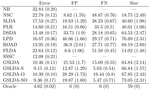
and standardize it such that the eigenvalues are between 0 and 1. Denote the 6th to 10th most connected nodes as J. The group means are generated such that µ(1)_j = 0.75 for allj ∈J and 0 otherwise; andµ(2)=−µ(1).

(41)

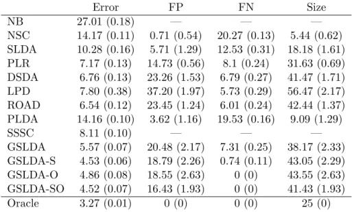
Table 2.1: Performance comparisons of different classification methods for Example 1.

Error FP FN Size

NB 27.01 (0.18) — — —

NSC 14.17 (0.11) 0.71 (0.54) 20.27 (0.13) 5.44 (0.62) SLDA 10.28 (0.16) 5.71 (1.29) 12.53 (0.31) 18.18 (1.61) PLR 7.17 (0.13) 14.73 (0.56) 8.1 (0.24) 31.63 (0.69) DSDA 6.76 (0.13) 23.26 (1.53) 6.79 (0.27) 41.47 (1.71) LPD 7.80 (0.38) 37.20 (1.97) 5.73 (0.29) 56.47 (2.17) ROAD 6.54 (0.12) 23.45 (1.24) 6.01 (0.24) 42.44 (1.37) PLDA 14.16 (0.10) 3.62 (1.16) 19.53 (0.16) 9.09 (1.29)

SSSC 8.11 (0.10) — — —

GSLDA 5.57 (0.07) 20.48 (2.17) 7.31 (0.25) 38.17 (2.33) GSLDA-S 4.53 (0.06) 18.79 (2.26) 0.74 (0.11) 43.05 (2.29) GSLDA-O 4.86 (0.08) 18.55 (2.63) 0 (0) 43.55 (2.63) GSLDA-SO 4.52 (0.07) 16.43 (1.93) 0 (0) 41.43 (1.93)

Oracle 3.27 (0.01) 0 (0) 0 (0) 25 (0)

and evaluate the performance, both prediction and selection accuracy, of all classification methods. Table A.1 in the Appendix displays the graph estimation accuracy for all examples.

Tables 2.1–2.4 give a summary of the performance comparison of all methods in Examples 1 and 4. In particular, misclassification rates in percentage (Error), false positives (FP) and false negatives (FN) of β estimation are computed. The misclassification rate is evaluated based on an independent test dataset of size 20,000. All metrics are averaged over 100 simulations and the numbers within parentheses are the standard errors. Both the NB and the SSSC are not considered in the comparison of variable selection, since these methods do not perform variable selection.

(42)

Error FP FN Size

NB 36.59 (0.43) — — —

SSSC 9.27 (0.17) — — —

GSLDA 6.60 (0.10) 25.48 (1.83) 15.41 (0.43) 49.07 (2.19) GSLDA-S 5.56 (0.07) 34.43 (2.52) 3.33 (0.41) 70.1 (2.77) GSLDA-O 6.19 (0.09) 27.26 (1.72) 7.37 (0.47) 58.89 (2.08) GSLDA-SO 5.79 (0.07) 30.78 (1.94) 2.16 (0.39) 67.62 (2.31)

Oracle 3.32 (0.01) 0 (0) 0 (0) 39 (0)

Error FP FN Size

NB 36.86 (0.80) — — —

SSSC 13.57 (0.91) — — —

GSLDA 10.53 (0.10) 27.34 (1.91) 36.67 (0.85) 56.67 (2.67) GSLDA-S 8.77 (0.08) 34.08 (2.77) 18.2 (0.72) 81.88 (3.37) GSLDA-O 9.77 (0.08) 36.87 (2.54) 26.22 (0.78) 76.65 (3.27) GSLDA-SO 8.91 (0.08) 35.17 (2.37) 16.31 (0.63) 84.86 (3.01)

Oracle 5.36 (0.02) 0 (0) 0 (0) 66 (0)

the GSLDA with an empty graph, it is a good benchmark to quantify the benefit of using graph structures. In most cases, the GSLDA provides better model selection than the DSDA. Therefore, utilizing the graph structure does help us to improve the LDA classifier in high dimensions.