Efficient techniques for end-to-end bandwidth estimation : performance evaluations and scalable deployment

(1)

Efficient Techniques for End-to-end Bandwidth Estimation: Performance Evaluations and Scalable Deployment

Alok Shriram

A dissertation submitted to the faculty of the University of North Carolina at Chapel Hill in partial fulfillment of the requirements for the degree of Doctor of Philosophy in the Department of Computer Science.

Chapel Hill 2009

Approved by:

(2)

(3)

ABSTRACT

ALOK SHRIRAM: Efficient Techniques for End-to-end Bandwidth Estimation: Performance Evaluations and Scalable Deployment.

(Under the direction of Jasleen Kaur)

Several applications, services, and protocols are conjectured to benefit from the knowledge of the end-to-end available bandwidth on a given Internet path. Unfortunately, despite the availability of several bandwidth estimation techniques, there has been only a limited adoption of these in contemporary applications. We identify two issues that contribute to this state of affairs. First, there is a lack of comprehensive evaluations that can help application developers in calibrating the relative performance of these tools—this is especially limiting since the performance of these tools depends on algorithmic, implementation, as well as temporal aspects of probing for available bandwidth. Second, most existing bandwidth estimation tools impose a large probing overhead on the paths over which bandwidth is measured. This can be a significant deterrent for deploying these tools in distributed infrastructures that need to measure bandwidth on several paths periodically.

In this dissertation, we address the two issues raised above by making the following contributions:

• We conduct the first comprehensive black-box evaluation of a large suite of prominent available bandwidth estimation tools on a high-speed network. In this evaluation, we also illustrate the impact that technological and implementation limitations can have on the performance of bandwidth-estimation tools.

• We conduct the first comprehensive evaluation of available bandwidth estimation algorithms, independent of systemic and implementation biases. In this evaluation, we also illustrate the impact temporal factor such as measurement timescales have on the observed relative performance of bandwidth-estimation tools. • We demonstrate that temporal properties can significantly impact the AB estimation process. We redesign the interfaces of existing bandwidth-estimation tools to allow temporal parameters to be explicitly specified and controlled.

(4)

(5)

LIST OF TABLES

1.1 Performance characteristics of an ABET . . . 11

1.2 Table of notations . . . 15

2.1 Available Bandwidth Estimation Tools . . . 20

3.1 Summary of wide-area bandwidth measurements (“f”= produced no data). . . 45

4.1 Data sets used . . . 51

4.2 Abilene: AB variability metrics . . . 60

4.3 UNC: AB variability metrics . . . 60

4.4 Stability in AB . . . 64

5.1 Traces used for evaluations . . . 70

(10)

LIST OF FIGURES

1.1 Illustration of end-to-end AB . . . 3

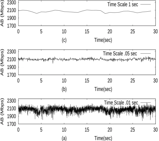
1.2 AB process observed on an Internet link over the same 30 sec interval at different timescales. . . 5

1.3 Internet Architecture . . . 12

2.1 Illustration of an Internet path . . . 17

2.2 Internet Architecture . . . 18

2.3 Impact of Interrupt Coalescence. (Graph from [PJD04]) . . . 24

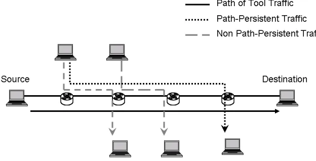
2.4 Illustration of Path-Persistent and Non-Path persistent traffic patterns . . . 28

3.1 Bandwidth Estimation Testbed. . . 34

3.2 CCDF of packet IAT distribution. . . 36

3.3 Comparison of /ab measurements on a 4-hop OC48/GigE with synthesized cross-traffic . . . 37

3.4 Comparison of ABET measurements on a 4-hop OC48/GigE path played back real traffic. . . . 40

3.5 Performance of iperf on a 4-hop OC48/GigE path with played back real traffic. . . 41

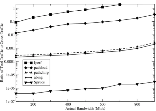
3.6 Tool overhead vs. available bandwidth. . . 42

3.7 Real world experiment conducted on the Abilene network . . . 44

3.8 Real world experiment conducted on the Abilene network for spruce. . . 45

4.1 Factors Affecting the AB process . . . 49

4.2 Sampling strategies. . . 53

4.3 Sampling Strategy vs. Accuracy (Mbps) . . . 54

4.4 CDF of Inaccuracies with different sampling strategies . . . 55

4.5 Impact of MT on accuracy . . . 55

4.6 Sampling Accuracy vs. SI . . . 56

4.7 RT vs. Inaccuracy (Mbps) . . . 57

4.8 Run-Time vs. Accuracy . . . 58

4.9 AB process observed at link during same 30 s window at different MT . . . 59

4.10 Impact of RT on range and standard deviation of AB . . . 61

4.11 Impact of MT and RT on variability . . . 62

(11)

5.1 Topology with a Single Bottleneck Link . . . 69

5.2 Validation of ABET Implementations . . . 69

5.3 Tool errors with default parameters . . . 71

5.4 Impact of MT, SI, and RTT . . . 72

5.5 Different tight and narrow links . . . 73

5.6 Performance with multiple bottleneck links (MT=50ms, SI=0.1) . . . 74

5.7 Single narrow link; two tight links . . . 75

5.8 Costs of ABETs with the Ibiblio trace (numbers in parenthesis indicate the MT in ms) . . . 76

5.9 CDF of response times with default parameters . . . 79

6.1 Location of Bottleneck Links . . . 89

6.2 Probe Overhead . . . 94

6.3 Path-based clustering: Actual vs. Inferred AB . . . 95

6.4 Distribution of Inference Errors . . . 96

6.5 Impact ofmon Inference Accuracy . . . 97

6.6 Distribution of Inference Errors with Capacity Substitution . . . 97

6.7 Performance of Consistently Rate Limited Paths . . . 98

6.8 Using Capacity-inference to Filter Out Ill-formed Tuples . . . 99

(12)

CHAPTER 1 Introduction

1.1 Motivation

Why measure end-to-end available bandwidth? The Internet provides a best-effort service model—applications that transfer data over the Internet are provided no guarantees or even apriori knowledge about the end-to-end performance that their transfers should expect. Such knowledge, if available, can help applications in better aligning their configuration and data transmission with the current state of network resources. Consequently, many applications rely on mechanisms or protocols that probe network paths to estimate the level of end-to-end transfer performance that a given network path can provide.

Over the past two decades, there has been significant interest in designing mechanisms for specifically probing for the packet delay and packet loss characteristics of Internet paths, and in using these to help guide data transport by Internet applications [BOP94, AGKT98, AP99]. More recently, with the emergence of data-intensive applications and increasing deployment of broadband access networks, there is a growing need to focus on yet another characteristic that applications are likely to be interested in—that of the transfer rate that can be obtained on a given path. The end-to-end available bandwidth (AB)—which represents the maximum spare ca-pacity available among all links of a given path—has emerged as a prime metric of choice for such applications. Several application domains are conjectured to benefit from the knowledge of this quantity:

• Congestion-control Protocols: A key objective of congestion-control protocols is to determine the

maxi-mum rate at which data can be transferred over a given path without overloading the network resources. It can be clearly seen that such a rate would be the maximum of the spare bandwidth available across all links on the path—consequently, efficient mechanisms for estimating the end-to-end AB can be quite useful for guiding such protocols.

• Video Streaming Protocols: Video-streaming applications often adapt the bit-rate of the video-stream by

(13)

supported on a given network path [BGMS04, FBB01]. Efficient mechanisms that continually estimate the end-to-end AB can help reconfigure the encoding parameters adaptively.

• Audio Streaming: Some applications require only a low, but consistent bit-rate—for instance, audio

streaming generates data at a nearly constant rate of 50-100 Kbps and works well only when the path can support the rate [Mos08]. Even such applications can benefit from the knowledge of end-to-end AB in order to decide, for instance, if a new client request for an audio stream can be served (given characteristics of the AB on the Internet path from the server to the client).

• Server Selection: For content-based services, in which a desired content may be available at several

servers, the knowledge of the end-to-end AB on the paths from each server to a given client can help the client select the best server to download from—this is especially useful for clients interested in down-loading large files or streams.

• Overlay Routing: With the emergence of multi-homing and overlay infrastructures [ABKM01, AMS+03, RK03], applications can now choose to transfer data over alternate paths different from the default Internet path to a destination. The selection of an alternate path can be better informed using the knowledge of end-to-end AB on each candidate path.

Each of the above applications would benefit from efficient techniques that probe for the end-to-end AB on a given set of path(s).

The dilemma: which probing technique?! Several sophisticated techniques have been developed in recent literature for measuring end-to-end AB on a given network path [JD02b, Rib03, SKK03a, Nav03, HS03, CC96a, ipe, KV06]. Unfortunately, there has been only a limited adoption of these techniques in Internet protocols/services. Indeed, most applications continue to use legacy mechanisms available prior to the emergence of these tech-niques. We believe that there are two key reasons for this state of affairs. First, there is a lack of compre-hensive evaluations of these techniques—consequently, it is not clear which techniques (if any) are efficient and well-suited for a given application. Second, many of the recently-developed techniques rely on sending large amounts of probe traffic for accurately estimating end-to-end AB. The associated overhead and latency of probing—especially when used in popular services/protocols—acts as a significant deterrent for protocol design-ers [SMH+05].

(14)

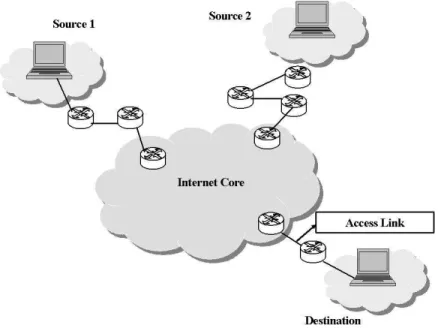
Figure 1.1: Illustration of end-to-end AB

1.2 Dissertation Goals

We begin by first formally defining the concept of end-to-end available bandwidth and identifying the require-ments from tools used for estimating it.

1.2.1 Requirements from ABETs

End-to-end available bandwidth (AB) represents the maximum spare capacity available among all links of a given path. Formally, the per-hop bandwidth available onithlink of a path,ABi, is defined as:

ABi[t1, t2] =Ci−

Bi(t1, t2)

(t2−t1)

(1.1)

whereABi[t1, t2]is the spare bandwidth available on the linkiover the time interval[t1, t2],Ciis the

transmis-sion capacity of linki, andBi(t1, t2)is the total traffic transmitted on the link during[t1, t2]. The end-to-end

available bandwidth of a network path is defined as the minimum of the spare bandwidth available at each of the constituent links of the path:

ABe2e= min

i∈[1,N]{ABi} (1.2)

For instance, in Fig 1.1, the end-to-end AB is 50 Mbps.

AB estimation tools, henceforth also referred to as ABETs , are designed to estimate the end-to-end AB on a given network path. Some distributed applications—such as overlay routing and server selection—also attempt to simultaneously employ such tools on multiple paths. Several key requirements guide the design of ABETs :

• High Estimation Accuracy: Each of the example applications listed before would be able to make optimal

(15)

underes-timation of end-to-end AB would prevent video-streaming applications and congestion-control protocols from, respectively, maximizing application quality and throughput—while overestimation of AB would drive network resources into a persistently overloaded state for the duration of the transfers.

• Small Response Time: AB on a given link can vary significantly over time—Fig 1.2, which plots the AB

observed on a production Internet link during a 30-second interval, illustrates this. Consequently, many applications—such as video streaming and congestion-control protocols—would need to continuously estimate up-to-date values of AB and adapt their transmission behavior accordingly. An ABET with a large response time would deliver only stale (and possibly invalid) values of AB to the associated application, thus impairing application performance.

• Low Probing Overhead: In order to prevent interference with transmission of useful application data,

ABETs should themselves rely on sending few probes into the network. Furthermore, a high probing overhead would be a significant deterrent to the widespread adoption of these techniques in popular Inter-net protocols and services.

1.2.2 (Limitations of the) State of the Art

Lack of Comprehensive Evaluations Several tools (ABETs ) have been proposed in recent literature for

actively probing for the end-to-end AB on a given network path [CC96a, HS03, JD02b, Rib03, SKK03a, Jin04, MBG00, Nav03]. These tools typically operate by injecting specially-designed streams of probe packets onto the path, observing the end-to-end delays experienced by the probe packets, and then estimating the end-to-end AB from the observations—details can be found in Chapter 2. Unfortunately, it is not clear how well these tools meet the above requirements. Specifically, existing evaluations of ABETs suffer from the following fundamental limitations.

(16)

1700

1900

2100

2300

0

5

10

15

20

25

30

AB (Mbps)

(a) Time(sec)

Time Scale .01 sec

1700

1900

2100

2300

0

5

10

15

20

25

30

AB (Mbps)

(b) Time(sec)

Time Scale .05 sec

1700

1900

2100

2300

0

5

10

15

20

25

30

AB (Mbps)

(c) Time(sec)

Time Scale 1 sec

(17)

results are often not comprehensive and get inadvertently biased toward highlighting the salient features of the proposed tool. This state of affairs leads us to our first goal:

It is important to conduct comprehensive evaluations of prominent AB estimation tools

under a common set of diverse network and traffic settings.

2. In current high-speed networks, variations in end-to-end delays may have an order of magnitude in the sub-millisecond range. Since most ABETs rely on measuring delay variations, high resolution and accu-racy in time-stamping probe packets is crucial for ensuring the accuaccu-racy of the inferred AB. Current PC platforms, however, are incapable of guaranteeing high time resolution due to multi-tasking and the use of mechanisms such as interrupt coalescence [JD02b]. Some tool implementers work around this limitation by relying on statistical filtering and smoothing techniques, but others do not—the use of such techniques does impact tool performance significantly [AMPR03, JT03].

It is important to note that the above implementation techniques are highly technology-specific. As tech-nology improves [PV02a], the impact of these techniques on ABET performance is likely to diminish. It is, therefore, natural to ask the question: what is the extent to which current implementation technology limits tool performance? In particular, how well would tool designs—including the design of their

probe-streams and inference logic—perform if technology advances in the future? This leads us to our second

goal:

It is important to evaluate, in an implementation-agnostic manner,

the algorithmic aspects of prominent ABETs .

3. Existing ABET designs focus primarily on, and differ most significantly in, the construction of probe streams and in the logic used to estimate AB from the observed delays. Most tool designs, however, seem to ignore three central temporal quantities related to measurement of the AB process—that of the measurement time-scale, the sampling intensity and strategies, and the probing duration. In particular, most existing ABETs do not allow the choice of these quantities and little is known about the impact of these quantities on the performance characteristics of an ABET. This leads us to our third goal:

It is important to study the impact of probing-related temporal quantities—including the measurement

(18)

In summary, our first set of objectives are concerned with evaluating ABETs under diverse settings of network, traffic, and temporal conditions.

Significant Overhead in Multi-path Application Domains Another fundamental issue with the state-of-the-art in ABET design is the large overhead when these tools are deployed in services such as overlay routing or server selection, that need to measure AB simultaneously on multiple paths. A naive approach for such services would be to run an instance of the tool on each of theN2_{paths in an}_N_{-node overlay infrastructure. However,}

such an approach suffers from two significant limitations:

1. High Overhead: Even with a low overhead tool, a single measurement of the AB may inject on the order of several megabytes of traffic into the network. ConductingN2_{measurements, would significantly overload}

the network path, especially as the number of nodes in the overlay infrastructure increases.

2. High Response-Time: ABETs can interfere with each other if run simultaneously on paths that share congested links. Hence, for the set of paths that interfere with each other, the measurements need to be run sequentially. In the worst case runningN2_{measurements sequentially would fundamentally limit the}

frequency with which the AB information for all paths can be updated. The above limitations lead to our final goal:

It is important to design a scalable AB monitoring scheme for distributed infrastructures, in which the number

of measurements that need to be made scale well with the size of the infrastructure.

In this dissertation, we pursue the four goals identified above by: (i) conducting a systematic evaluation of

implementations of prominent ABETs ; (ii) studying the impact of temporal factors on the AB estimation

pro-cess; (iii) conducting an implementation-agnostic evaluation of the AB estimation techniques; and (iv) designing a scalable AB estimation scheme for simultaneous and distributed monitoring of multiple paths. In what follows, we briefly summarize the approach and main results for each of these—the details follow in subsequent chapters.

1.3 Goal 1: Black-box Evaluation of ABET Implementations

(19)

the network speeds to which these implementations can scale—this is because at high speeds, the lack of high-precision and accurate timers on current PC platforms could impair the performance of such tools. Our hope is to identify tool implementations that are suitable for contemporary application domains.

Approach With the above goals in mind, we conduct ABET evaluations under each of the following scenarios: • On a high-speed network test-bed with commercial routers and switches, with constant bit-rate cross

traf-fic.

• On a high-speed network test-bed with commercial routers and switches, with traces of representative traffic collected from production Internet links and replayed as cross-traffic on the test-bed.

• On an Internet2 gigabit network path between Sunnyvale and Atlanta against real cross-traffic flowing on the path—the actual AB was verified using SNMP counters on the network path.

• On the Internet path between San Diego Supercomputing center and Oak-Ridge National Laboratories, where actual AB was unavailable but the relative performance of the tools was studied.

Summary of Results Some highlights of the findings of our evaluation can be summarized as follows:

1. Tools utilizing packet-pair techniques like Abing and Spruce should be aware of delay quantization possi-bly present in the networks.

2. AB can not be measured reliably in gigabit high-speed networks using 1500 Byte MTUs and with only microsecond time-stamp resolution.

3. ABETs should also be able to detect, and perform well in, the presence of interrupt coalescence.

4. TCP-based bandwidth estimation schemes like Iperf perform well, but even an approximately 1% packet loss can severly affect AB estimates.

1.4 Goal 2: Impact of Temporal Factors on AB Estimation

(20)

• Measurement Timescale: A critical parameter in the definition of AB in Equation (1.1) is the length,

(t2−t1), of the time interval over which it is observed—we refer to this quantity as the measurement

timescale (MT). In Fig 1.2, we plot the time-series of AB, observed at three different timescales of10ms, 50ms, and1s, during the same 30 s observation period on an Internet link. We observe that the AB process

can appear quite different depending on the timescale at which it is observed. In particular, it is likely that the MT impacts the accuracy as well as variability of the AB measured by a given ABET. Consequently, any application that relies on such a tool would want the tool to measure AB at an MT relevant to the application domain. For instance, while a large-file-transfer application is likely to be interested in only the average AB obtainable at super-second timescales, a media-streaming application is likely to also be interested in knowing the small-timescale variations in AB.

• Measurement Duration (Run-time): Run-time (RT) refers to the length of the time interval over which

several samples of the AB process are collected, and used to infer properties of the AB process. In practical terms, the run-time is the total time taken by a tool from invocation to reporting an AB estimate. This includes the time taken for sending several probe streams (each of which potentially returns one sample of AB), and converging on an AB estimate.

The most significant impact of run-time on AB measurement is in terms of its robustness and its variability. While a shorter run-time is likely to yield samples more consistent with each other, longer run-times are more likely to yield a sufficient number of samples for reliably estimating the mean as well as variability in the AB process.

• Sampling Intensity and Strategy: Given an observation timescale, the AB process consists of a series of

back-to-back readings of AB observed within a given time interval. ABETs essentially only sub-sample this AB process. Existing tools differ in the fraction of the AB process—henceforth, referred to as the

sampling intensity (SI)—that they sample during the tool run-time. Existing tools also differ in their sam-pling strategy—the manner in which AB samples are collected from within a given time interval [CPB93].

The sampling strategy and the fraction of the AB process sampled are likely to impact the accuracy of estimating the mean AB in a given time interval. For instance, larger is the sampling rate, better is likely to be the AB estimation accuracy; however, greater would be the network overhead.

(21)

(i) How does the choice of sampling strategy, sampling intensity, MT and RT impact the accuracy of the esti-mated AB? (ii) How does the choice of MT and RT affect the variability of the measured AB? (iii) How stable is AB in the post-measurement periods? Answering these questions reveals the impact that the above mentioned temporal parameters have on the performance characteristics of the ABETs .

Evaluation Approach As mentioned before, existing ABETs differ significantly in the design of their probe streams and inference logic. In order to answer the questions raised above in a manner independent of these choices, we assume the existence of a perfect tool that can estimate the end-to-end AB perfectly. This assump-tion lets us study the impact of the above-identified (currently) design-agnostic quantities—namely, run-time, measurement timescale, and sampling intensity and strategy—while isolating the analysis from the impact of design-dependent factors. It also lets us adopt a passive trace-analysis based approach for answering the above questions. With such an approach, it is possible for us to compute the ground truth about the AB process.

We conduct passive analysis of link-level traces collected from several types of production Internet links.

Summary of Results The main findings of our evaluation can be summarized as follows:

1. The choice of the measurement timescale does not impact the accuracy as long as the sampling intensity is held constant.

2. Sampling more that 30% of the AB process does not yield a significant improvement in the accuracy of the AB estimate.

3. The AB process shows significant variability at timescales of less than 50 ms, which corresponds to send-ing a large train of packets rather than packet-pairs.

4. Back-to-back measurements of the AB do not change significantly, which can be exploited for predictive purposes in applications that need to continuously estimate AB.

1.5 Goal 3: Implementation-agnostic Evaluation of ABETs

(22)

environment gives us the ability to create a technologically-perfect network where (i) fine-grained clock granu-larity is achievable on end-systems, (ii) interrupt coalescence effects do not occur, (iii) packet losses do not occur and, (iv) buffer sizes are unlimited. Second, we design a common implementation framework for instantiating prominent ABETs in NS-2—a common framework helps us avoid any bias due to differences in implementation efficiencies. It also allows us to enhance existing interfaces for all ABETs to enable controlling the measurement timescale and sampling intensity. We extract implementation details from the publicly available versions of the tools and the publications that describe them, and implement these within our framework. We then evaluate the ABETs under diverse settings of traffic and network conditions, including: (i) single-hop topologies with constant-bit-rate as well as dynamic and representative cross-traffic, (ii) multi-hop topologies with multiple tight and/or narrow links, and (iii) on topologies with a representative mix of responsive cross-traffic. We study several performance characteristics (Table 1.1) of the ABETs .

Performance Parameter Description

Accuracy Difference between the actual and measured AB Overhead Traffic injected by ABET to make single AB measurement Intrusiveness Rate of traffic injected by ABET to make single AB measurement

Run-Time Time taken to make a single AB measurement Perturbation Impact on response times of TCP flows

Table 1.1: Performance characteristics of an ABET

Summary of Results The main findings of our evaluation can be summarized as follows:

1. Increasing the MT improves the accuracy of the estimates. However, the gains in accuracy are negligible beyond a timescale of 50 ms.

2. Increasing the SI has no impact on the accuracy of the AB estimates.

3. As the MT increases the run-time of a tool also increases.

(23)

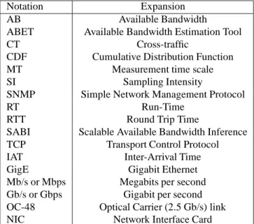
Figure 1.3: Internet Architecture

1.6 Goal 4: Scalable AB Inference for Overlays

In order to design a scheme, which can give us completeN2_{path AB without making}_N2_{measurements we rely}

on two key insights about the Internet

1. Sharing of the access hops: Most of the Internet architecture is structured as illustrated in Fig 1.3. End-nodes either lie within enterprise networks or metropolitan-area networks belonging to local Internet Ser-vice Providers (ISPs). These edge networks are then connected via access links to other ISPs that comprise the core of the Internet—these include major Tier-1 and Tier-2 ISPs. Let the access segment of an end-node refer to the sequence of edge hops and links that connect it to the Internet core. The connectivity structure of the Internet then implies that the paths from any two given source nodes, S1 andS2, to a

common destinationDare likely to share the access segment ofD(see Fig 1.3).1

2. Bottlenecks lie close to edges: Recent Internet-wide measurement studies have reported that the bottleneck links of most end-to-end network paths lie close to the end-nodes, and are likely to be the access/peering links between customers and ISPs [Li05, RRB04]. This essentially implies that the bottleneck link of a path is likely to lie on the access segments of either end-nodes.

(24)

LetAB(i, j)denote the end-to-end AB on the path from nodeitoj. We defineABin

i to be the minimum of

the AB on all links in the access segment of nodei, in the direction of carrying traffic from the core to the node i, andABout

i to be the minimum AB on these links, in the direction of carrying traffic from nodeito the Internet

core (see Fig 1.3). The two observations made above then collectively imply that the end-to-end AB on the path between two given nodes,S1andD1, can be approximated as:

AB(S1, D1) ≃ min{ABoutS1 , AB

in

D1} (1.3)

The above formulation can be used to infer the AB on the path betweenS1andD1without necessarily directly

measuringAB(S1, D1).

Since we know that access hops are shared, we can reduce the measurements that need to be made by clustering nodes together which share the same access segments to the rest of the nodes in the network. Once we have created these clusters, a representative node in a cluster can measure theABin

Di of all the nodes outside the

cluster. The other nodes in the group can measureABout

Sj to their representative node. We can then use Equation

1.3 to infer the end-to-end AB between any two nodes. We propose three variants of this basic approach that offer a trade-off between estimation accuracy and probing overhead—the most scalable variant incurs an overhead only linear in complexity to the size of the overlay.

We evaluate our approaches on the PlanetLab infrastructure [Pla] by relying on the S3 monitoring ser-vice [YSB+06]. Our evaluation shows that our approach can estimate AB with an estimation accuracy within 20% for a majority of the estimates—this significantly outperforms the accuracy of existing schemes.

1.7 Thesis Statement

In this dissertation, we demonstrate that:

1. It is possible to isolate and study the temporal and algorithmic aspects of AB estimation.

2. Contemporary implementations of system timers and interrupt coalescence can significantly impair the performance of an otherwise sound AB estimation logic.

(25)

4. ABETs based on the probe-rate model are more robust to traffic and path dynamics.

5. It is possible to design a scalable inference scheme, that helps achieve desirable operating points on the trade-off between accuracy and overhead, for collectively monitoring the AB on all paths in a distributed overlay network.

1.8 Summary of Contributions

The major contributions of this thesis can be summarized as follows:

• We conduct the first comprehensive black-box evaluation of a large suite of prominent AB estimation tools on a high-speed network. In this evaluation, we also illustrate the impact that technological and implementation limitations can have on the performance of ABETs .

• We conduct the first comprehensive evaluation of AB estimation algorithms, independent of systemic and implementation biases. In this evaluation, we also illustrate the impact temporal factor such as measure-ment timescales have on the observed relative performance of ABETs .

• We demonstrate that temporal properties can significantly impact the AB estimation process. We redesign the interfaces of existing ABETs to allow temporal parameters to be explicitly specified and controlled. • We design AB inference schemes which can be used to scalably and collaboratively infer the AB for a

large set of end-to-end paths. These schemes allow an operator to select the desired operating point in the trade-off between accuracy and overhead of AB estimation. We further demonstrate that in order to monitor the AB on all paths of a network we do not need access to per-hop AB estimates and can simply rely on end-to-end AB estimates.

1.9 Roadmap

(26)

our scalable AB monitoring approach in an overlay network. We conclude with Chapter 7 by outlining future work and our conclusions.

1.10 Notations

In the rest of this dissertation, we will rely on the following notations.

Notation Expansion

AB Available Bandwidth

ABET Available Bandwidth Estimation Tool

CT Cross-traffic

CDF Cumulative Distribution Function

MT Measurement time scale

SI Sampling Intensity

SNMP Simple Network Management Protocol

RT Run-Time

RTT Round Trip Time

SABI Scalable Available Bandwidth Inference

TCP Transport Control Protocol

IAT Inter-Arrival Time

GigE Gigabit Ethernet

Mb/s or Mbps Megabits per second Gb/s or Gbps Gigabit per second OC-48 Optical Carrier (2.5 Gb/s) link

NIC Network Interface Card

(27)

CHAPTER 2 Design of Bandwidth estimation tools

The area of AB estimation has been an active area of research for the past few years. In this chapter we summarize related work that studies several aspects of the AB estimation problem. We first examine techniques that were developed to estimate the bottleneck capacity on an to-end path. We next discuss tools for estimating end-to-end AB. Next we examine past evaluations of AB estimation tools as well as formal analysis geared towards better understanding the performance parameters of AB estimation tools. Finally we examine methodologies that have been proposed to efficiently monitor large overlay networks.

2.1 Background

We start with some definitions and observations that will be used in this chapter.

End-to-end Bottleneck Capacity The transmission capacity of a link refers to the speed at which data can be transmitted on the link. If the transmission capacity of a link is 1 Mbps, then it follows that the maximum amount of data that can be transmitted on the link in a single second is106_{bits. Alternatively, the time taken to}

transmit a single bit is 1µs.

Given an Internet path consisting of several links, the end-to-end bottleneck capacity refers to the minimum of the transmission capacities of all the constituent links of the path. Formally, if the path consists ofnlinks and Ciis the transmission capacity of theithlink, then the bottleneck capacity of the path is defined as:

min

1≤i≤n{Ci} (2.1)

(28)

Figure 2.1: Illustration of an Internet path

End-to-end Available Bandwidth The end-to-end AB was formally defined in Section 1.2.1. Informally, it represents the minimum of the spare bandwidth available over all links of a path. The link with the least amount of spare bandwidth is commonly referred to as the tight link [JD02a].

In Figure 2.1, the end-to-end available bandwidth is 50 Mbps and the first link is the narrow link. In this example, the tight and narrow links are different.

Multi-homing in Access Networks At this point it would be prudent to make some observations about the structure of the Internet (Figure 2.2). The Internet is organized in a hierarchical structure of tiered Internet Service Providers (ISPs), that cooperate with each other based on either a customer-subscriber model or a peer-to-peer model, in order to transfer data between two end nodes. Tier-1 [tie] service providers operate large networks and provide long haul connectivity over large geographical areas—contemporary examples include Verizon, Sprint, and AT&T. Tier-1 service providers typically have peering relationships with one another which allows them to exchange data on a no-cost basis with each other. One layer below in the hierarchy are tier-2 service providers, which are predominantly regional in geographical scope. Such providers may have peering relationships with other tier-2 service providers, but also have customer-provider relationships with tier-1 ISPs in order to use the latter to send or receive customer data. Finally, tier-3 ISPs interact with other providers almost exclusively based on the customer-provider model. Since tier-3 networks are often used to provide Internet access to customers, we also refer to these as access networks.

(29)

Figure 2.2: Internet Architecture

would be useful in making such decisions.

2.2 Capacity estimation tools

A seminal paper in the area of per-link capacity estimation was by Van Jacobson who proposed a tool called

Pathchar[Jac]. Pathchar estimates per-hop capacity by using the Variable Packet Size (VPS) probing

methodol-ogy, that relies on using probe packets of different sizes to estimate the capacity of every hop along a path. Let us consider a path withKhops, and assume that the capacity of theithlink isCibits per second (bps)—thus,

the time taken to transmit a packet of size L bits on theithlink will be _CL_i seconds. Now, the time taken for a

L-bit packet to travel from the sender to theithhop and back can be expressed as:

Ti(L) = i

X

k=1

(L Ci

+Queuingf wd+P ropagationf wd+Queuingrev+P ropagationrev+

L Ci

) (2.2)

whereQueuingf wd andQueuingrev are the delays experienced by waiting in the queue of theithlink on

(30)

either direction of link i. Finally, _CL

i is the time taken to transmit the packet on the link.

Most per-hop capacity estimation tools rely on a time-to-live (TTL) limiting mechanism. Every packet sent on the Internet has a TTL field that is initialized by the sender. At every router that the packet traverses, this TTL field is decremented by one. If a router receives a packet where the TTL is zero, it discards the packet—most routers also send an Internet Control Message Protocol (ICMP) packet, which is typically 64 bytes, back to the sender. Thus if we limit the TTL of a packet toi, then we can force theithrouter to send back a constant size

ICMP message to the sender—this mechanism can yield the information needed to computeTi(L). So the above

equation now becomes:

Ti(L) = i

X

k=1

(L Ci

+Queuingf wd+P ropagationf wd+Queuingrev+P ropagationrev+

Licmp

Ci

) (2.3)

Now if we send a large number of probe packets to hopi, we would expect that the packet with the lowestTi(L)

would experience no queuing delay in the forward and the reverse path. From this, Equation 2.3 can be simplified as:

Ti(L) = i

X

k=1

(L Ci

+P ropagationf wd+P ropagationrev+i

Licmp

Ci

) (2.4)

Now since theP ropagationf wd,P ropagationrev, andLicmpare constants, Equation 2.4 reduces to:

Ti(L) =K+ i X k=1 (L Ci ) (2.5)

whereK=P ropagationf wd+P ropagationrev+Licmp_C_i . The equation now has the formF(L) =K+Mi∗L,

whereMiisPik=1 1

Ci andF(L)isTi(L). Now if we were to measureMi by using packets of different sizes,

thenCi= _M_i₊₁1−Mi.

Using the above relation, the capacity of all the hops of a path can be measured. Mah et. al. [Mah00] designed an improvement for Pathchar, which used linear regression to better estimate the values ofMi. Downey[Dow99]

(31)

order to estimate the capacity of the end-to-end path. The principle behind this approach is that two packets sent back-to-back will arrive at receiver with a spacing between them which is proportional to the capacity of the path between them. This spacing between the packets is referred to as the dispersion of the packet-train. Formally specified, the dispersion is defined as followsTdisp =_C_end−Lto−end. Pathrate uses a system of creating histogram

and studying the most frequently occurring modes in the histogram in order to estimate the value ofTdisp and

then compute the end-to-end capacity.

We next discuss tool that were designed for estimating the available bandwidth (versus bottleneck capacity) on an Internet path or link.

Tool Probe Stream Inference Metric

Pathload [JD02b] Equi-Spaced Train One-way Delay Pathchirp [Rib03] Exponential spacing Dispersion Spruce [SKK03a] Packet-Pair Dispersion Abing [Nav03] Packet-Pair Dispersion

IGI [HS03] Packet Train Dispersion

Iperf [ipe] TCP-Stream Throughput

Cprobe [CC96a] Packet Train Receiving Rate Table 2.1: Available Bandwidth Estimation Tools

2.3 AB Estimation Tools

2.3.1 End-to-End AB estimation tools

Table 2.1 lists some prominent AB estimation tools. All AB estimation tools work under the same underlying principle which involves sending probe packets at well defined and known intervals on an Internet path, such that they temporarily induce a load on the path. This load will cause the existing cross traffic on the path to be interspersed by the probe packets. When these probe packets reach the other end of the path (receiver), the receiver studies how the intervals between the probe packets has changed and compares these intervals to the known intervals between the probe packets when the probe packets were initially sent. Using empirical or analytic techniques, the AB of the end-to-end path can then be computed. We will discuss the details of some of the prominent tools next.

• Pathload[JD02b] reports the AB using two thresholds, theupperrangeandlowerrangeAB, which

(32)

to be 0 and theupperrangeto be the capacity of the end-to-end path. It then sends out a stream at an initial

guess of the AB. The one-way delay in the stream is analyzed to study if this stream rate was greater than or less than the AB. If the AB is exceeded theupperrangeis set to the current sending rate of the stream.

If the AB is not exceeded, thelowerrangeis set to the current sending rate. The rate of the next stream

is then determined by using the relation upperrange+lowerrange

2 . This process continues iteratively, till the

difference between theupperrangeand thelowerrangebecomes less than a certain threshold. At this point

the currentupperrangeandlowerrangeare reported as the AB.

• PathChirp[RRB+03] uses an exponentially spaced packet train to estimate the AB. It uses a parameter called the spread factor, which defines the exponent of the Chirp train. For instance if the spread factor is 2, a 5 packet Chirp would send the first two packet spaced at 1 Mbps, the third at 2 Mbps, the fourth at 4 Mbps and the fifth at 8 Mbps. The Chirp is analyzed at the receiver end to study at which rates in the Chirp the sending rate was greater than the receiving rate. The principle being that since a Chirp covers a wide range of rates, the rates after which the AB is exceeded will be characterized by the sending rate being greater that the receiving rate. Thus we can infer the AB of an end-to-end path by observing these points of change. Multiple chirps are used in order to improve the confidence of the estimates.

• IGI/PTR[HS03] sends a train of back-to-back packets to the receiver which is used to estimate the path

capacity. It then uses the path capacity as its first sending rate to the receiver. The gaps at the source and the gaps at the destination are compared to infer if the current sending rate was greater than the AB . If so the current sending rate is reduced by a constant decrease factor that can be specified during the tool run, and this process is continued till the point where the receiver reports that the source gaps and the destination gaps are equal. It is at this point that IGI and PTR differ. IGI estimates the cross-traffic rate using the difference in the gap values. It then subtracts this estimate of the cross-traffic rate from the bottleneck link capacity to infer the end-to-end available bandwidth. PTR on the other hand compute the average receiving rate of the stream and infers that as the AB of the path.

• Abing[Nav03] and Spruce[SKK03b] use a packet-pair based technique to estimate the AB. The sender

sends two packet spacedδin=_CS seconds apart; where S is the packet size and C is the link capacity. The

receiver then observes the spacing between the packets when it arrives at the receiver and computes the dispersion in order to compute the AB by using the following relationAB=C×(1−δout−δin

δin ). Where

(33)

using a Poisson process, Abing sends packet-pairs periodically.

• Iperf [ipe] is a standard benchmarking and monitoring tool. It can be used to compute the throughput of a

path by actually running a TCP connection on the path. While it has been shown that the TCP throughput of an end-to-end path is not the same as the AB [DJ03], Iperf continues to be a popular choice among network operators for measuring the AB.

• Abget[DMA+06] and QuickProbe[KV06] are variants of the Pathload tool. Abget uses a TCP

connec-tion to measure the AB down-stream AB on a path by controlling the acknowledgments that the client receives in order to control the rate at which the server sends data. This method of controlling the rate of an incoming packet stream is then used to implement the Pathload logic and the inference is carried out in the same manner as described above. QuickProbe another variant of Pathload reduces the time-taken by Pathload to make an inference by reducing the number of packets that are required to make an inference. • Cprobe[CC96a] first finds the end-to-end capacity of a given path using another tool called Bprobe[CC96a].

It then sends a packet train at that rate to the destination host. The rate at which this stream is received at the other end of the path is inferred to be the AB.

Most ABET designs as observed above focus on the construction of the probe-streams and the logic used to estimate the AB from the observed delays. However, these tool designs ignore two central temporal quantities related to the measurement of the AB process: the MT and the SI . Thus it is important to redesign the ABET interfaces to allow the choice of MT and SI, and study the impact of these on ABET performance.

In this thesis in order to study the impact that the observation time-scale and the sampling frequency have

on the accuracy of the tool, we redesign the tool interfaces such that we can set the observation time-scale and

sampling frequency. We can then evaluate the tools under the same conditions and compare their performance.

2.3.2 Per-hop AB estimation tools

In the recent past another class of AB estimation tools have been proposed which measure the AB on every hop of a path. Two prominent tools in this domain are Pathneck and Stab.

Stab[RRB04] works on a principle similar to PathChirp. However here every packet in PathChirp is

(34)

to be a measurement packet. In order to measure the AB up-to theith_{hop on a path, the load packets have in}

every packet-pair have their TTL set to i. The MP train is sent in exactly the same manner as PathChirp. The intuition behind this approach is that the load packets will create the excursion patterns at any given hop, which will also be reflected in the small-sized measurement packet, since the measurement packets will always queue up behind the the load packets. When a MP reaches theith_{hop, all the load packets will be dropped (because}

they are TTL limited), and the measurement packet which reflect the spacing of the load packets when they were dropped will carry on to the receiver. The receiver can infer the AB of theithhop using the same inference logic

as PathChirp. This procedure is done for every hop, to get a per-hop estimate of the AB .

Pathneck[Li05] uses a stream construction called a Recursive Packet Train (RPT). A recursive packet train

consists of two components (i) A Load Train and (ii) A Measurement Train. A single RPT is constructed as follows the first k packets are TTL limited measurement packets with small size and are sent back-to-back. The next L packets are large load packets, which are sent at a rate specified by the IGI/PTR algorithm. The final k packets are also TTL limited load packets. The first and last measurement packet have a TTL of 1, the second and second last measurement packet have a TTL of 2 and so on for all the k measurement packets. In the case of Pathneck is set to 30 and L is set to 70, though these are parameters and can be varied. The intuition behind Pathneck working is as follows. As the RPT traverses the path, at each successive hop the first and the last packet of the RPT will be dropped and a TTL expired message will be sent back to the receiver. By observing the dispersions of the TTL limited packets, the amount of time the load packets were queued at a particular hop can be computed, which using IGI/PTR inference logic can give us information about the AB on a given hop.

In this thesis we show that scalable approaches to monitoring the AB in a network can be done using

end-to-end AB estimation tools. We show that other approaches[HS05] which require per-hop AB information are less

accurate than our method and also do not perform as well as existing end-to-end AB estimation tools.

2.3.3 Implementation techniques to achieve high time-stamping accuracy

(35)

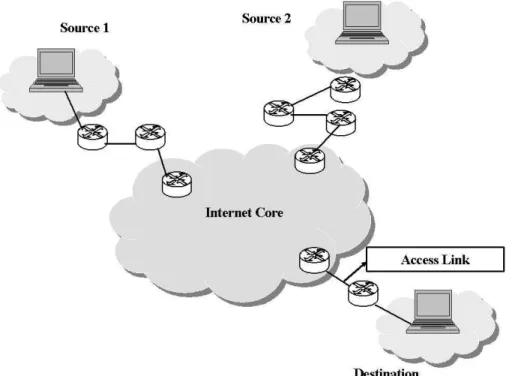
Figure 2.3: Impact of Interrupt Coalescence. (Graph from [PJD04])

unable to make a distinction between packet-pairs sent at rate _CB

r and∞. Most tool implementers work around

this limitation using two techniques [JD02b, Rib03, SKK03a]: (i) they rely on OS support for detecting and discarding probe streams that appear to not have been time-stamped accurately; and (ii) they collect observations from several probe streams before converging on a robust estimate of AB. While such implementation techniques do not differ much across current ABETs, these do impact tool performance significantly [AMPR03, JT03]. It is important to note that the above techniques are highly technology-specific. As technology improves [PV02a], the impact of these techniques on ABET performance is likely to diminish.

Existing tools differ in the efficiency with which such systemic biases are handled. For instance in [PJD04] the authors propose a technique which can be used to detect interrupt coalescence. They propose that the graph of the one-way delays of a large stream of packets being affected by interrupt coalescence would look like an increasing saw-tooth function when it was received at the destination machine. Figure 2.3 taken from [PJD04] illustrates this effect. This is because packets will be buffered at the card till an interrupt timer expires and all the buffered packets will be delivered back-to-back to the kernel and then the application. In such a scenario, only the last packet of every burst should be considered since it has the most current timing information and has suffered from the least buffering at the NIC.

(36)

tools suffer from biases introduced by interrupt coalescence. In this thesis, we evaluate some prominent AB

estimation tools in an environment where systemic effects like interrupt coalescence could come into play. We

then study how the ABETs could be impacted by these effects and correlate our findings to other studies which

have focused specifically on these issues.

2.4 Tool Evaluation

Several tool proponents compare the performance of their tools against that of others under controlled lab set-tings as well as in Internet-wide experiments [HS03, Rib03, SKK03a]. Ribeiro et. al. [Rib03] compare the performance of PathChirp to that of Pathload [JD02b] and TOPP [MBG00] in an emulated lab setting. They find that PathChirp is more accurate than TOPP and less intrusive than Pathload. Hu et. al. [HS03] compare the performance of IGI/PTR to that of Pathload and Iperf on 13 Internet paths of capacity within 100 Mbps. They observe that while the readings of the three tools match on some paths, they fluctuate on other. Since the actual AB of these paths were not known, tool accuracy was not verified. Strauss et. al. [SKK03a] compare the performance of Spruce to that of Pathload and IGI. They use SNMP data collected at five minute intervals to evaluate the accuracy of these tools on two 100 Mbps paths. They also compare the sensitivity of the tools to changes in AB by performing several experiments on the RON testbed. They find that IGI is inaccurate at high loads, and Spruce is more accurate and less intrusive than Pathload. Coccetti et. al. [CP02] evaluate early ABETs, including Iperf and Pathload, on a low speed (less than 4 Mbps) 4-5 hop topology with and without cross-traffic. They conclude that tool results strongly depend on configuration of the router queues and that a considerable amount of care would need to be taken while interpreting the results from any ABET, especially if QoS features were present in the network. In [LRL04], the authors analyze at large time-scales, the performance of several bandwidth estimators that can be represented mathematically. Unfortunately, their evaluation consid-ers only low-bandwidth paths with a single bottleneck link. Furthermore, several iterative estimators cannot be represented using their formulation.

(37)

in high-speed networks, or when the tight and narrow links are different.1 _{As a result of these practices, the} results are often not comprehensive and get inadvertently biased toward highlighting the salient features of the proposed tool.

As listed in Section 1, there are a wide variety of factors that could impact the accuracy and performance parameters of an ABET. Unfortunately there are no evaluation studies that systematically evaluate all the

param-eters that can influence the performance of a given ABET. Furthermore no evaluations take into consideration

the temporal aspect of the process of AB estimation and the impact that it could have on the tools accuracy.

To summarize, existing ABET evaluations are either biased by limitations of current implementation technology and/or are not comprehensive in evaluating tools against diverse network,probing, systemic and temporal condi-tions. In this thesis we study the factors that can affect the performance of an ABET and systematically quantify

the impact that they have on the performance parameters of ABETs.

2.5 Formal analysis of AB estimation tools

In order to better understand the performance bounds of AB estimation tools, there have also been several efforts to quantify the biases and the errors that can be observed by the various AB tools and techniques.

In [LRLL04] the authors analyze the performance of AB estimation tools on a single-hop path. They assume a simple FIFO model of queuing and derive the ”Response Curve” of an input probe that is used to estimate the AB . The response curve is the function that relates the input gaps to the output gap on a single-hop path as a function of the cross-traffic intensity and link capacity that is present on that path. The authors derive an expression which given an input gap,cross-traffic intensity, probe packet size and link capacity can define bounds for the expected gap values. The difference between the actual output gap response curve and the theoretical lower bound of the response curve is defined as the probing bias, which directly relates to the amount by which the cross-traffic process is being changed because of the external probes that we are introducing into the network. The authors also conclude that using a longer probing packet train or larger packet sizes, would reduce the probing bias.

In [LRL05] the authors extend the single-hop model into the more general case model of a multi-hop path and formulate a ”Response Curve” for a multi-hop path using a fluid cross-traffic model. They conclude, that the for a multi-hop path, that the relation between the input and output gap (Response Curve) is a continuous

1_{The tight link of a path is one with the least amount of available bandwidth, while the narrow link is the one with the least transmission}

(38)

piecewise linear function. The first point of slope change is analytically shown to be the point at which the AB of the path is obtained. They then extend the fluid-cross traffic model to a more realistic cross-traffic model and show that the response curve for the realistic cross-traffic model is lower bounded by the its fluid counterpart. They also analytically show that as the packet size or the packet train length approaches infinity, the bias terms approaches 0. That is theoretically we can obtain perfect knowledge of the AB if we can send arbitrarily large packets or arbitrarily long packet trains.

In [LFV07b] the authors model an end-to-end path and an AB estimator on that path as a min-plus system, in the context of network calculus. The primary assertion behind this approach is that it is possible to completely describe a min-plus system by using only its impulse response. An impulse response of a system is the response of a system when the input to the system is the burst function, which in the context of AB estimation is a probe stream which has an instantaneous rate of infinity Mbps. This impulse response is also defined as the service curve of the system. Thus the objective of the Min-plus analysis is that given an arrival function and a departure function which can be obtained by observations, can we obtain the service curve of the end-to-end path (Min-plus system). The authors show analytically that it is not possible to get the exact service curve, and therefore derive an expression to find the service curve which maximally lower bounds the actual service curve. The authors then show how this formulation can be used in passive monitoring, rate scanning and Chirps to obtain a lower bound on the service curve and hence infer the AB on that path.

In [LDS06] the authors analytically study the performance of AB estimation tools, specifically the perfor-mance of the packet-pair techniques. They show that even in the case where there is a single bottleneck link and the situation where the narrow link and the tight-link are the same there are situations where the packet-pair technique will result in an underestimation of the AB. In the case of path-persistent (Refer to Figure 2.5) cross-traffic the estimator that is used in the packet-pair method can accurately measure the AB. However in situations where the cross-traffic is not path-persistent, the packet-pair estimator will always underestimate the AB when the sending rate is greater than the AB.

In this thesis we empirically study the issues of bias that are introduced by varying network conditions and

cross-traffic interaction models in ABETs and verify many of the observations made in the theoretical models

(39)

Figure 2.4: Illustration of Path-Persistent and Non-Path persistent traffic patterns

2.6 Efficient Network Monitoring

Recent work has addressed the issue of monitoring of all links of a given network in a scalable manner. Most approaches rely on the observation that many end-to-end paths in a network share several links—this redundancy can be exploited to drastically reduce the number of end-nodes used for probing links as well as the number of probes sent by these. The reduction problem has been modeled by many as a vertex-cover problem. [BCG+01] optimizes the number of SNMP probes that need to be sent to NetFlow-enabled routers to query for the link utilization and the latency. The authors provide a generic heuristic algorithm, which produces a near optimal set of links that need to be monitored. [KK06] optimizes the problem of beacon placement in the presence of dynamic IP routes, such that each link of a give network can be deterministically monitored for link failures and delays, while placing a minimum number of probing beacons. [CKC05] measure the delay and loss efficiently by using a linear-algebraic approach for selecting a subset of links, and then inferring the network properties from this subset. [SQZ06] uses a Bayesian network based approach to monitor the delay, capacity and loss in an efficient manner.

(40)

tool in order to monitor the all-pairs AB in a scalable manner. The algorithm relies on a series of landmark nodes to which Pathneck[HLM+04]; a tool to locate the bottleneck on an Internet path; is run. Pathneck also provides lower bounds on the per-hop AB. Every node monitors the per-hop AB on its ingress and egress links to a series of landmark nodes. When the AB between any two nodes is required the system will take the minimum of the AB at the sources egress links and the destinations ingress link and infer the end-to-end AB as the minimum of those two ABs. Evaluation of this scheme demonstrated that the AB estimation accuracy is less than 50% for 80% of the cases. In this thesis we design a scalable AB monitoring infrastructure, which reduces the number of

measurements and shows better inference accuracy than previously proposed schemes.

2.7 Network aware application designs

There are many applications that make network aware decisions. For instance the Resilient Overlay Network (RON) [ABKM01] monitors the delay and bandwidth on its networks and is able to provide delay or loss op-timized paths as required. Multimedia applications like [NN98] also rely on the delay information in order to construct their multi-cast routing tree. The knowledge of the delay is also useful in web caching [WY00] where the latency is used a metric to decide where a some content should be cached. The objective of this system is to cache data at geographically proximate locations, such that requests can be responded to with minimum delay. Peer-to-Peer like Bit-torrent [Bit] can also make intelligent choices about peers as studied in [Qur04]. Despite there being many potential AB aware applications, it is not clear what the performance gains would be on using an AB aware application.

(41)

and the capacity to determine what the output rate of the streaming protocol should be. As can be observed there are several potential applications that could benefit from the knowledge of the AB. However there is no clear quantification as to what performance improvements could be obtained by using an AB aware application. In

this thesis we design an infrastructure that can monitor the AB of a network, which would give the above listed

(42)

CHAPTER 3 Evaluation of ABET implementations

We begin our series of evaluations by first evaluating publicly-available implementations of ABETs—in this first study, we treat each of these tools as a black-box and evaluate the default design choices along the algorithmic, implementation-related, and sampling-related temporal dimensions. A major focus of our analysis in this chapter is to understand the extent to which systemic issues and implementation efficiencies impact tool performance— the impact of temporal and algorithmic factors is studied in subsequent chapters.

ABETs face increasingly difficult measurement challenges as link speeds increase. Consider the issue of time precision: on faster links, time-gaps between packets decrease, rendering packet probe measurements more sensitive to timing errors. Available bandwidth measurements on high-speed links stress the limits of clock precision especially since additional timing errors may arise due to the NIC itself, the operating system, or the Network Time Protocol (designed to synchronize clocks of computers over a network) [PV02b]. Additionally, mechanisms such as interrupt coalescence that are used to improve network packet processing efficiency, mislead end-to-end tools that assume uniform per-packet processing and timing [PJD04].

On the other hand, ABETs are being increasingly deployed in high-speed network settings such as the Net-work Weather Service [Wol98] and the TeraGrid [Ter] infrastructure. Since the systemic issues mentioned above play a greater role in high-speed networks, it is critical to develop an understanding of the performance of promi-nent ABETs in such environments. Unfortunately, as described in Chapter 2, most past evaluations of ABETs have been restricted to paths with capacities of 100 Mbps or less—furthermore, these evaluations are often not comprehensive in the set of tools evaluated.

(43)

in the test-bed setting. This implies that the results we obtain here are generalizable to the performance of the ABETs in actual deployments. It also presents strong motivations for designing and testing ABETs in high-speed testbeds similar to the one that we will describe in this chapter before deploying them on live systems.

3.1 Background: Interrupt Coalescence and network measurements

We first discuss how interrupt coalescence can impact network measurement and specifically AB estimation. Jain et. al. [PJD04] have conducted an in-depth analysis of this issue. Recall from Chapter 2 that AB estimation tools send a series of probe packets with a controlled and pre-determined spacing between them on the path of interest, and the receiver studies changes in the inter-packet gaps in order to make an inference about the AB . Clearly, ensuring high precision time-stamping and accurate spacing between the packets is critical for obtaining an accurate estimate of the AB.

To put this in context, in order to achieve a data rate of 1 Gbps, a 1500 byte packet would have to be transmitted (and received) every 12 µs. On general-purpose machines, packet transmissions and receipt by a network interface card (NIC) is handled by means of triggering interrupts—for instance, when a packet is received, the current process running on the CPU is interrupted, context is saved, and the packet is processed before returning the context to the original process. This processing and the associated context switch can be fairly costly operations to perform. Modern systems, consequently, reduce the overhead by grouping together packets that arrive close in time, and use a single interrupt to trigger their processing. This process is known as Interrupt coalescence (IC).

Efficient techniques for end-to-end bandwidth estimation : performance evaluations and scalable deployment

ABSTRACT

Table of Contents

LIST OF TABLES

LIST OF FIGURES

CHAPTER 1

Introduction

1.1

Motivation

1.2

Dissertation Goals

1.2.1

Requirements from ABETs

1.2.2

(Limitations of the) State of the Art

1700

1900

2100

2300

0

5

10

15

20

25

30

(a) Time(sec)

Time Scale .01 sec

1700

1900

2100

2300

0

5

10

15

20

25

30

(b) Time(sec)

Time Scale .05 sec

1700

1900

2100

2300

0

5

10

15

20

25

30

(c) Time(sec)

Time Scale 1 sec

1.3

Goal 1: Black-box Evaluation of ABET Implementations

1.4

Goal 2: Impact of Temporal Factors on AB Estimation

1.5

Goal 3: Implementation-agnostic Evaluation of ABETs

1.6

Goal 4: Scalable AB Inference for Overlays

1.7

Thesis Statement

1.8

Summary of Contributions

1.9

Roadmap

1.10

Notations

CHAPTER 2

Design of Bandwidth estimation tools

2.1

Background

2.2

Capacity estimation tools

2.3

AB Estimation Tools

2.3.1

End-to-End AB estimation tools