Combining Input Output (IO) analysis with Global Vector Autoregressive (GVAR) modeling: Evidence for the USA (1992 2006)

(1)

Combining Input-Output (IO) analysis

with Global Vector Autoregressive

(GVAR) modeling: Evidence for the

USA (1992-2006)

Konstantakis, Konstantinos and Michaelides, Panayotis G.

National Technical University of Athens

2014

Online at

https://mpra.ub.uni-muenchen.de/67111/

(2)

Combining Input-Output (IO) analysis with Global Vector

Autoregressive (GVAR) modeling: Evidence for the USA (1992-2006)

Konstantinos N. Konstantakis and Panayotis G. Michaelides

National Technical University of Athens, Greece

Abstract: The purpose of this paper is to assess the interdependencies among the eight (8) main sectors of economic activity in the US economy, using quarterly data on output and labor fora period of fifteen years (1992-2006), just before the first signs of the global recession made their appearance. In this context, we set up a novel methodological framework which combines Input-Output (IO) analysis with state of the art Global Vector Autoregressive (GVAR) modeling. In addition, we use the IO matrices to provide a procedure in order to test for the existence of dominant sector(s) in the USA and estimate a GVAR model with dominant sector(s) and the exogenous variables of Global Credit and Global Trade acting as the transmission channels. Our results seem to suggest that the US economy has relatively limited connectivity, in terms of sectoral output and

labor, among the various sectors.

Keywords: GVAR, Input Output, US sectors, Weight Matrix



The authors would like to thank Theodore Mariolis for a fruitful discussion. Corresponding author: Panayotis G. Michaelides, Assistant Professor of Economics_{, Laboratory of Theoretical and Applied Economics, School of Applied}

(3)

1. Introduction

The VAR approach and especially the Global VAR (GVAR) model, provide

nowadays a very useful framework for assessing the transmission of shocks among

economic entities.1_{The GVAR framework was introduced by Pesaran et}_al._{(2004) and}

developed through several quality theoretical contributions such as Pesaran and Smith

(2006), Dées et al. (2007b) Chudik and Pesaran (2011a), (2011b) as well as empirical ones

such as Dées et al. (2005), (2007a), Pesaran et al. (2006), Pesaran et al. (2007), Bussière et

al. (2012), Konstantakis and Michaelides (2014).

The GVAR model is suitable for assessing relationships between economic

entities while its methodology provides a general, yet practical, modeling framework for

the quantitative analysis of the relative importance of different shocks and channels of

transmission. In fact, it consists of a compact econometric model of the economic

entities involved which is specifically designed to model the economic interdependencies

among economic entities, e.g. at both the national and international level.

The GVAR framework is structured upon observables, which typically include

economic aggregates, trade and financial variables, with other unit-specific variables

serving as proxies for common unobserved factors. It is exactly this characteristic that

constitutes an important input in the so-called “decoupling” of the US sectoral economy.

The purpose of this paper is to assess the interdependencies among the eight (8) main sectors of economic activity in the US economy, using quarterly data on output and labor for a period of fifteen years (1992-2006), just before the first signs of the global recession made their appearance.

(4)

We have chosen the variables of output and labor because they are probably the major economic variables at the sectoral level which are able to express, in a nutshell, the economic conditions of each sector. More precisely, we take into consideration the production of each sector through the variable of output as well as the main factor of production (i.e. input) through the variable of labor. Additionally, we have chosen to use the variables of Global Trade and Global Credit instead of their domestic counterparts i.e. US Credit and US Trade, due to the high degree of opennessof the US economy.

The present paper is the first, to the best of our knowledge, which provides a simple and practical framework for applying the GVAR approach at the sectoral level. In this framework, we propose combining the traditional Input Output (IO) Leontief methodology with the state of the art GVAR approach. To this end, we set out a detailed methodological framework for constructing the sectoral weight matrix of the GVAR model, which builds on the IO technical coefficients matrix. Next, we provide a procedure in order to test for the existence of dominant entities and we implement the proposed novel sectoral methodology to the US economy.

The proposed framework which combines the traditional IO methodology with the state of the art GVAR modeling has considerable advantages with respect to either of the two approaches upon whichit builds. With respect to the GVAR approach, the weight matrix constructed in this work,which is derived based on Leontief’s IOmatrix,is perfectly capable of capturing the linkages between the various sectors of the economy. Hence, the modeling of the economy is complete since there are no missing relationships due to the fact that all sectors are explicitly included in the GVAR model. With respect to the IO approach, our proposed framework acts as a state of the art econometric technique which is capable of producing robust statistical estimates based on real–world

data on economic aggregates instead of mere point calculations, while incorporating the

(5)

The remainder of the paper is structured as follows: section 2 sets out the proposed methodology, section 3 presents the data and the variables; section 4 describes the empirical analysis; section 5 presents the estimation results; section 6 offers a brief discussion; finally, section 7 concludes.

2. Methodology

2.1 GVAR Analysis

The Global VAR model consists of eight (8) major economic entities, namely the eight

economic sectors of the US economy. Each sector i, 1, 2, … , 8 follows a VAR

model, augmented by the so-called exogenous variables of global trade (T) and credit

(D), expressing the transmission channels through which the various economic

transactions and shocks take place. The endogenous variables denote a 8×2 vector of

macroeconomic variables belonging to each sector i, consisting of the sectoral Output

(Y) and Labor (L).

We use the variables of output and labor as the model’s endogenous variables because they are probably the major economic variables at the sectoral level which are able to express, in a nutshell, the economic conditions of each sector. In fact, we take into consideration the production of each sector through the variable of output as well as the main factor of production (i.e. input) of each sector through the variable of labor.

The foreign variables ∗_, represent a weighted average of the other sectors’

variables that are regarded to be weakly exogenous in each sector’s model, whose weights

are pre-determined. Mathematically, the VAR model for each sector is:

, , ∗ [1]

For 1, 2, … ,8 1. . . . where is the set of sectoral domestic

(6)

is a vector of fixed intercept; is a set of the Global Variables and is a vector of

their respective coefficients ∗ is the set of weighted foreign variables and

, is the matrix of lag polynomial of the associated coefficients.Matrix is a8 × 8

dimensional matrix of weights and ~ . . 0, with mean zero and the

variance-covariance matrix Σi.

The implementation of the GVAR methodology has two steps. Firstly, each

sector’s VARX model is constructed treating the variables of global Trade and global

Credit as exogenous. After the construction of each VARX model we relate their

corresponding estimates through link matrices by stacking them together to obtain our

GVAR model. In particular, we consider the following model for country i:

∗ ∗ [2]

To begin with, we group all foreign and domestic variables together as:

∗ Therefore, for each sector i the respective model becomes:

. .

where: , _, _, , .

By gathering all the domestic endogenous variables together, we define the

following global vector and we obtain the identity: , ∀ 1, …,8

where W is the weight matrix. Thus, by using the former identity in the i-thsector-

specific model, we get:

, , ,

By combining each sector model with the later equation weobtain the GVAR:

, , ,

(7)

If the M matrix is non-singular, then we obtain the reduced form of the GVAR

model:

, ,

where: . and

Furthermore, following Chudik and Smith (2013), in the potential presence of a

dominant entity we transform each i-thVARX model of the GVAR to account for this

dominant sectoras follows2_:

, , , ∗, , ∗, [3]

where _, _, , _, is a 2x1 vector of variables of the dominant sector and

={1,..7}.

We examine the dynamic characteristic of our GVAR model through the

so-called Generalized Impulse Response Functions (GIRFs) following Koop et al. (1996)

and Pesaran and Shin (1998).Analytically, a positive standard error (σ) unit shock is

examined on every variable in the universe of our model aiming at determining the

extent to which each economic sector, responds to a shock. Also, we study the extent to

which these shocks have persistent effects. The (Generalized) Impulse Response

Function (GIRF) is as follows:

/ _∀ _{1, 2, …}_[4]

where is the Impulse Response Function n periods after a positive standard error

unit shock; is the jth row and jth column element of the variance–covariance matrix

Σ of the lower Cholesky decomposition matrix of the error term which is assumed to be

2_{Note that despite the insightful suggestion by Chudik and Smith (2013) to use a dominant entity, they do}

(8)

normally distributed; B is the coefficients’ matrix when inversely expressing the VAR

model as an equivalent MA process and is the column vector of a unity matrix. See

further Koop et al. (1996) and Pesaran and Shin (1998).

2.2 Input Output Analysis

(A) Constructing the sectoral weight matrix in an IO framework

Ιn the core of the GVAR methodologyat the international level is the so-called trade weight matrix(see e.g. the seminal work by Pesaran et al. 2004). To this end, we use the IOmatrix3 of the US economy to serve as the means to create the sectoral weight matrix4.

As is well known, the IO model is based on the following equation for the

various (n) economic sectors:

= + + ... + + , i= 1, 2, ..., n[5]

where: ≥0 is the output of sector i, is the final demand for the product of sector i,

is the product of sector i used by sector j.

Equation (5) can be written as follows, in matrix form:

Χ = ΑΧ + Υ[6]

where: X is the vector of outputs, Y is the vector of final demand, and A is the so-called

input or technicalcoefficients matrix whose typical element is equal to:

[7]

where: ≥0 is interpreted as the quantity of output from sector i required to produce

one unitof output in sector j.

Solving the balance equation [6] for X, we obtain:

3

Instead of the standard technical coefficients matrix A, we could also use the tailored hybrid technology-based product IO tables constructed in the spirit of Rueda-Cantuche and ten Raa (2013).

4

(9)

X = Y[8]

in which is then × n identity matrix, is the so-called Leontief inverse and Y is the column vector of final demand.

As we know, in the IO approach, the main tools of analysis are the technical

coefficients matrix A and the Leontief inversematrix , namely the matrix of

input-output multipliers of changes in final demand into levels of outputs.

Now, based on the fundamental IO matrix of technical coefficients A, we

constructmatrix , which has the following form:

≡ ⋮ …⋱ ⋮

…

where each element of is given by the expression:

≡ [9]

and the element of matrix expresses the product of sector i that is used from sector

j, is the total output of the j-th sector and is interpreted as the quantity of output

from sector i required to produce one unit of output in sector j, as we have seen earlier.

Notice that, in general, , ∀ , ∈ 1, … , .

In the IO matrix , the row elements express the quantities of goods and

services, in value terms, supplied by one sector to itself and all others. Similarly, column

elements express quantities obtained by a sector from itself and all others. In general,

(10)

Next, we construct the transpose of matrix Q, i.e. . In matrix , the row

elements express quantities obtained by a sector from itself and all other sectors, whereas

the column elements express quantities supplied by a sector to itself and all others.

Now, let matrix P be defined as the difference between matrix Q and its

transpose, , or in matrix notation:

≡

Thus, the typical element, , of matrix P is equal to :

≡

Each element, , measures the net amount of goods and services of a sector, in value

terms, that flows between itself and each other sector, in a respective year.

Obviously, P is a matrix with zeros in the main diagonal. In matrix form:

≡ 0⋮ …⋱ ⋮

… 0

since, by definition, every element of its main diagonalindicates the quantities that each

sector obtains and supplies to itself, which, in a general equilibrium framework, are equal

to each other. Hence, 0, , ∀ , ∈ 1, … , . Apparently, P

represents a net (intermediate) intra-sectoral flow matrix.

Since we are interested in constructing the so-called weight matrix, close to the

spirit of the GVAR model at the international level (Pesaran et al.2004), we proceed as

follows:Let NQ, be the IO matrix whose typical element, , is given by the following

expression:

(11)

A net intra-sectoral flow weight is defined as the ratio of flows of goods and services

between sector i and sector j, over the total absolute flows of goods and services realized

by sector i. Or in mathematical terms:

≡_∑ [11]

Obviously, W is a matrix with zeros in the main diagonal. Or, in matrix form:

≡ 0⋮ …⋱ ⋮

… 0

since 0 as discussed above, and, in general, , ∀ .

For instance, the element indicates the flows of goods and services, between

sector 1 and sector 2 as a proportion of the total flows of sector 1.

Apparently, W represents an intermediate net intra-sectoral flow weight matrix.

Ιf the net intra-sectoral flow weights of a sector tend to remain stable over time

this would imply a situation of structural stability. On the other hand, if the weights were

found to be unstable over time, an instability situation might be indicated.

The proposed weights can be computed from the data contained in IO Tables

and National Accounts and the derived net intra-sectoral flow weight matrix W is directly

(12)

(B) Testing for Dominant Sector(s) in an IO framework

In order to test for the number of dominant sectors, wecalculate the eigenvalues of Input

Output matrix A5. However, in what follows, we focus on matrix Q(instead of A), since

its eigenvalue distribution expresses the dynamic behavior of any given economy in

terms of net intermediate intra-sectoral flows, which is the focus of our analysis.6The

eigenvalues λ(i), i=1,..,8 of matrix Q are such that | | 0 where is the n × n

identity matrix and each eigenvalue is considered to have multiplicity equal to 1. In

general: λ(i)=a ± bj, where j =-1, a, b ∈ , and the modulus of λ(i)is equal to:| |

√ 0, i=1,...,8.Now, let λ(pf) = λ(1) denote the Perron–Frobenius (P–F)

eigenvalue of the n × n matrix Q. We divide each eigenvalue’s modulus with the P-F

eigenvalue’s modulus to get the normalized eigenvalue: | | ⋅ | | ,

i=1,...,8. The normalized eigenvalues: ρ(i), i=2,...,8are the so-called non-dominant

eigenvalues, since ρ(pf)=ρ(1)=1.

Following common practice, the number of dominant sectors implied by the

economy’s structure is equal to i*, for which ρ(i*)>0.4-0.3 approximately,since values of

ρ(i*)less than 0.40–0.30 might be considered negligible from a practical point of view

(Mariolis and Tsoulfidis, 2014).

3. Data and Variables

We have chosen to apply the proposed methodology to the US economy because: (i) it is

the largest economy in the world in terms of output produced and, probably, (ii) the

world’s dominant economy in terms of power and influence. Also, the US economy

5_{An interesting approach would also be the investigation of a dominant region in the Input-Output}

multiregional analysis concept proposed by Canning (2013).

(13)

presents (iii) interesting connectivity among its economic sectors (e.g. Acemoglou et

al.2012), as well as (iv) very good data availability.

We use an eight-sector classification of the US economy because: (i) it avoids

large data requirements, a characteristic which is highly desirable for the expository

nature of our work, (ii) it avoids large computational complexity related to the already

heavy structure of the econometric representation of the GVAR model, (iii) it provides a

compact and practical representation of the country’s economy, and, (iv) it is consistent

with the findings by other researchers highlighting the need for compact classification

formats of the US economy (see e.g. Mariolis and Tsoulfidis, 2014). Our classification

builds on the respective compact US classification by the Bureau of Labor Statistics

(BLS) (2014) and the Canadian classification by the Canadian Industry Statistics (2012).

For the detailed industry classification, see Table A1 (Appendix).

The data are quarterly and stop in 2006, just before the first signs of the US

recession made their appearance. The model incorporates two (2) sector-specific variables: Output (Y) and Labor (L) that were obtained from the Bureau of Economic

Activity (BEA) and the Bureau of Labor Statistics (BLS), respectively.Regarding the

global variables, we use the aggregate values of (i) Global Trade and also (ii) Global

Credit, both in millions of dollars, which were obtained in constant prices from the

World Data Bank.

(14)

is considered to be the main locomotive of global demand of goods and services which in turn dictates the use of Global Trade; (c) an increasing percentage of US firms operate at a multinational level and thus they have access to financial markets around the globe and not only to the US market, which in turn implies that the use of Global Credit is preferable. Due to the openness of the US economy, we used IO matrices which contain information on both domestically produced as well as imported inputs, which is consistent with the spirit of the original GVAR model.7The Leontief Inverse matrices for the USA are those of years 1995, 2000 and 2005 and come from the OECD (STAN)

database.For the Leontief Inverse matrices in the adopted industry classification, see

Tables A2-A4.All variables are expressed in constant prices.

The weightsare computed using the detailed methodology set out earlier where -

for the calculation of the weights - the time span is split into three sub-periods (1992–

1997, 1998-2002 and 2003–2007) and for each sub-period we use a representative

domestic IO table, assuming that the production technology for the US remains constant

during the sub-periods.

4. Empirical Analysis

4.1 GVAR Empirical Analysis

Stationarity

A number of relevant econometric tests need to be carried out first. We start by testing

for stationarity based on the ADF methodology following Pesaran et al. (2004). In case

the time series employed are not stationary, we induce stationarity following, among

others, Koop (2013). As we know, there are several ways to test for the existence of a

unit root. In this paper, we use the popular Augmented Dickey-Fuller (ADF)

7

(15)

methodology (Dickey and Fuller. 1979) following Pesaran et al. (2004). The ADF test is

based on the following regression:

1 1

1 m

t t t

i

bt Y _ _

  _  _ 



    



 

[12]

whereΔ is the first difference operator, t the time and ε the error term:

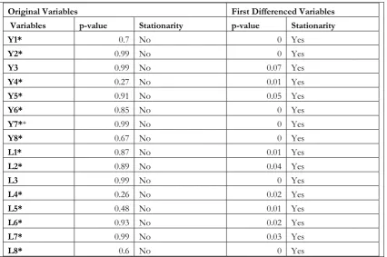
The original time series were found to be non-stationary. In fact, all the variables

were I(1). Thus, stationarity was induced by means of first differencing (Tables A5-A11).

Asymptotic Properties

For the purpose of estimation and inference in stationary models, Chudik and Pesaran

(2011a) showed that the relevant asymptotics are: → ∞[13]

where T denotes the time dimension and N is the number of endogenous variables in the

model. Our model clearly complies with thisasymptotic conditionT/N< ∞.

Cointegration

Also, we have to check for cointegration between the different variables that enter the

model. We employ the popular Johansen (1988) methodology that allows for more than

one cointegrating relationship, in contrast to other tests. The methodology is based on

the following equation: ∑ [14]

where: ∑ ∑ [15]

The existence of cointegration depends upon the rank of the coefficient matrix Π which

is tested through the likelihood ratio, namely the trace test described by the following

formulas: ∑ log 1 [16]

where: T is the sample size and is the largest canonical correlation.

The trace test tests the null hypothesis of r<n cointegrating vectors and the

(16)

The results of testing for cointegration, which are available upon request by the

authors, suggest that no cointegration is present in any of the US economic sectors

leading us to apply the GVAR methodology using a VARX model for each sector with

stationary variables, i.e. the first differences8_{enter the VARX model of each sector.}

4.2 Input Output Empirical Analysis

Testing for Dominant Sector(s)

Close to the spirit of Chudik and Smith (2013), we proceed by investigating the existence

of dominant sector(s) in the GVAR model. In this context, we divide each eigenvalue’s

modulus with the P-F eigenvalue’s modulus to get the normalized eigenvalue:

| | ⋅ | | , i=1,...,8. The normalized eigenvalues: ρ(i), i=2,...,8 are the so-called

non-dominant eigenvalues, since ρ(pf)=ρ(1)=1.

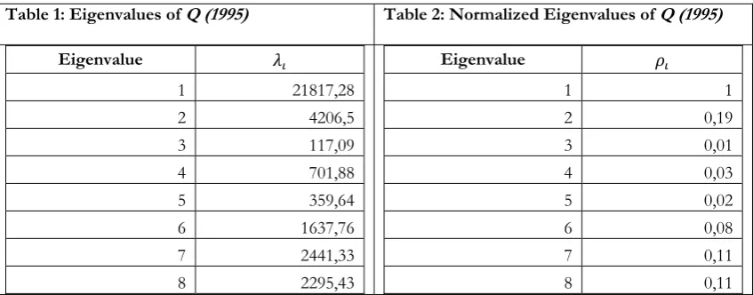
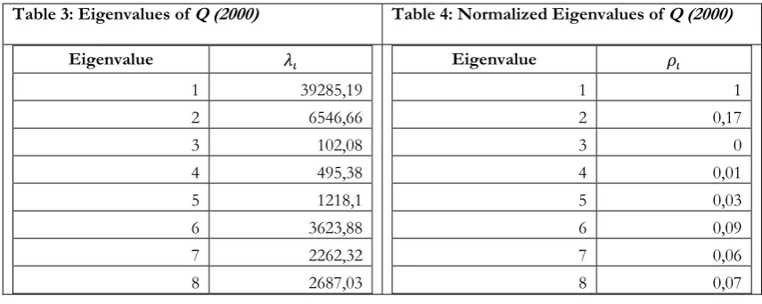
Tables 1,3 and 5 present the eigenvalues of the US matrix Q for the years

1995,2000 and 20059_{respectively, whereas Tables 2,4 and 6 presentthe normalized}

[image:16.595.87.511.504.670.2]

eigenvalues for the respective years.

Table 1: Eigenvalues of Q (1995) Table 2: Normalized Eigenvalues of Q (1995)

Eigenvalue

1 21817,28 2 4206,5

3 117,09 4 701,88 5 359,64 6 1637,76

7 2441,33 8 2295,43

Eigenvalue

1 1

2 0,19

3 0,01

4 0,03

5 0,02

6 0,08

7 0,11

8 0,11

8_{Of course, for the variables that were found to be I(2) we used second differences so as to ensure that all}

the variables in the model are stationary.

9_{The same procedure was applied to the technical coefficients matrix A for years 1995, 2000 and 2005, and}

(17)

[image:17.595.83.513.73.440.2]

Eigenvalue

1 39285,19 2 6546,66

3 102,08 4 495,38 5 1218,1 6 3623,88

7 2262,32 8 2687,03

Eigenvalue

1 1

2 0,17

3 0

4 0,01

5 0,03

6 0,09

7 0,06

8 0,07

Eigenvalue

1 7313.01 2 9930.26 3 9081.20 4 5932.55 5 184.24 6 3182.29 7 2102.92 8 741.30

Eigenvalue

1 1 2 0.14 3 0.13 4 0.08 5 0.02 6 0.04 7 0.03 8 0.01

Following common practice, the number of dominant sectors implied by the

economy’s structure is equal to i*, for which ρ(i*)>0.4-0.3 approximately, since values of

ρ(i*)less than 0.40–0.30 might be considered negligible from a practical point of view, as

we have seen earlier. Hence, the results of Tables 2,4 and 6 suggest the existence of

onedominant sector in the US economy, throughout the period of our investigation.

Constructing the sectoral weight matrix

Next, we proceed by constructing the weight matrix of our GVAR model using the

methodology described earlier. As we have seen, a net intra-sectoral flow weight matrix

W has the form:

0 …

⋮ ⋱ ⋮

[image:17.595.83.511.76.247.2]

(18)

since 0 as explained earlier and, in general, , ∀ . The typical element

is defined as the ratio of flows of goods and services between sector i and sector j,

over the total flows of goods and services realized by sector i: _∑

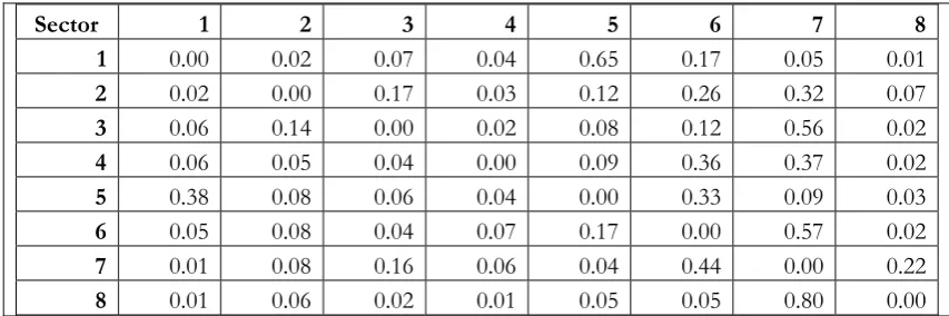
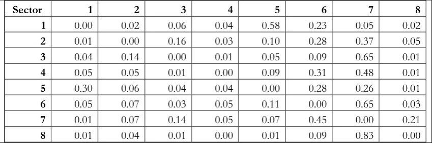
In our investigation, we construct three weight matrices for the years 1995, 2000

and 2005, respectively(see Tables 7-9), based on the IO inverse matrices for the US

economy (see Tables A2-A4, Appendix) and the respective flow matrices Q (see Tables

[image:18.595.84.512.336.488.2]

A12-A14, Appendix)

Table 7: Weight Matrix (1995)

Sector 1 2 3 4 5 6 7 8

1 0.00 0.02 0.05 0.03 0.53 0.20 0.16 0.00

2 0.02 0.00 0.16 0.02 0.20 0.34 0.18 0.07

3 0.01 0.03 0.00 0.02 0.03 0.05 0.83 0.03

4 0.03 0.01 0.08 0.00 0.02 0.08 0.71 0.07

5 0.23 0.07 0.07 0.01 0.00 0.35 0.25 0.02

6 0.04 0.05 0.04 0.02 0.14 0.00 0.67 0.05

7 0.02 0.01 0.40 0.09 0.06 0.37 0.00 0.05

8 0.00 0.05 0.13 0.08 0.03 0.23 0.47 0.00

Sector 1 2 3 4 5 6 7 8

1 0.00 0.02 0.07 0.04 0.65 0.17 0.05 0.01

2 0.02 0.00 0.17 0.03 0.12 0.26 0.32 0.07

3 0.06 0.14 0.00 0.02 0.08 0.12 0.56 0.02

4 0.06 0.05 0.04 0.00 0.09 0.36 0.37 0.02

5 0.38 0.08 0.06 0.04 0.00 0.33 0.09 0.03

6 0.05 0.08 0.04 0.07 0.17 0.00 0.57 0.02

7 0.01 0.08 0.16 0.06 0.04 0.44 0.00 0.22

[image:18.595.83.510.544.686.2]

(19)

[image:19.595.86.511.105.247.2]

Sector 1 2 3 4 5 6 7 8

1 0.00 0.02 0.06 0.04 0.58 0.23 0.05 0.02

2 0.01 0.00 0.16 0.03 0.10 0.28 0.37 0.05

3 0.04 0.14 0.00 0.01 0.05 0.09 0.65 0.01

4 0.05 0.05 0.01 0.00 0.09 0.31 0.48 0.01

5 0.30 0.06 0.04 0.04 0.00 0.28 0.26 0.01

6 0.05 0.07 0.03 0.05 0.11 0.00 0.65 0.03

7 0.01 0.07 0.14 0.05 0.07 0.45 0.00 0.21

8 0.01 0.04 0.01 0.00 0.01 0.09 0.83 0.00

As we have seen, if the net intra-sectoral flow weights of a sector tend to remain

stable over time this would imply a situation of structural stability. On the other hand, if

the weights were found to be unstable over time, an instability situation might be

indicated. Based on the calculated weight matrices, we find evidence of increased

structural stability over time, with very few exceptions.

By means of the matrices W we proceed with estimating the GVAR model, using

sector 7 (information technology, finance and communications), as the dominant sector

in the US economybecause: (a) it is the largest sector in terms of output produced, as

well as the (b) the largest sector in terms of the output exchanged.

5. Estimation Results and Stability

Next, for the implementation of our model we have to determine the optimum lag length

for each sector’s variables.

Optimum Lag Length of the GVAR model

We make use of the so-called Schwartz-Bayes Information criterion (SBIC) introduced

by Schwartz (1978), where the optimum lag length is given by the objective function:

(20)

where LL(k) is the log-likelihood function of a VAR(k) model, n is the number of

observations and k is the number of lags and k is the optimum lag length selected. As the

works of Breiman and Freedman (1983) and Speed and Yu (1992) have shown, SBIC is

an optimal selection criterion when used in finite samples.

The optimum lag length for each sector was equal to two (2) quarters (Pesaran et

al. 2005). Therefore, the VARX model for each sector , 7is as follows:

. ,

, , . , ,

. , ,

,

, ∑ , ,

.∗ , ∗ ,

. ∗ , ∗

[18]

while, for the dominant sector, i=7, its VARX model is the following:

.

, , ,

.

, ,

,

. ∗ , ∗ ,

. ∗ ,∗

where Δis the first differencing operator, _, , _, is the 1x2 vector representing

output and labor, respectively, for all sectors 1, … ,8, p is the lag length that is p=2,

, are the exogenous variables of global Trade and global Credit

with the respective coefficients, _, , _, and _, are the matrices of lagged polynomials,

, and , are the coefficient matrices of the dominant sector and the other sectors

respectively and _, is the intercept, while is a vector of idiosyncratic, serially

uncorrelated sector-specific shocks with mean zero and the variance-covariance matrix

Σi, ~ . . 0, .

The effect of the foreign variables on their sector-specific counterpart is

presented in Table A16, Appendix. The results suggest that in all sectors labor seems to

(21)

the dominant sector 7, as expected, appears to have the most significant interconnections

with the rest of the sectors, a fact that seems to be consistent with our choice of the

dominant sector. Additionally, we witness relatively limited interconnectivity among the

various sectors mainly with respect to their output, a fact which is consistent with the

findings by other researches (e.g. Mariolis and Tsoulfidis, 2014).

GVAR Stability Conditions

Also, in order to determine whether the model is stable, we have to check the stability of

the sector-by-sector models, separately. However, following Pesaran et al. (2004) and

Mutl (2009) it is not sufficient to examine the sector-by-sector stability, ignoring the

endogeneity of the other variables ∗ _, . Hence, it does not suffice to require that ρ( ) <

1 for stability, where ) is the spectral radius of the matrix , 1, … ,8. Instead,

Mutl (2009, p. 9) derived a sufficient condition for the model to be stable, namely that

the maximum absolute row sums of W are less or equal to , that is:

‖ ‖ [19]

where is the uniform bound of absolute row and column sums of the weight matrix

W: ∑ ∑ _, ∞[20]

where does not depend on T or N and the choice of indexes i and q, but can

potentially depend on other parameters of the model; and _, denotes the (q, m)-th

element of W .Finally, note that if r is the maximum number of eigenvalues of Φ, then

(22)

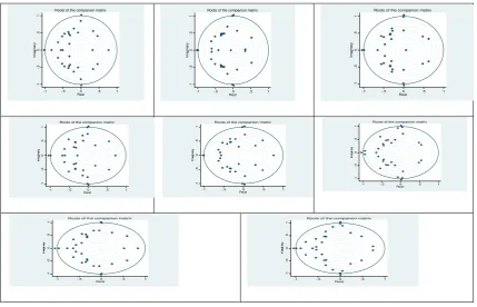
The results of our analysis are consistent with the stability of each sector’s VARX

model (see Figure 1), based on the eigenvalues lying on or inside the unit circle, and

[image:22.595.84.514.183.459.2]

imply stability of the estimated model and of the various sectors of the US economy.

Figure 1: Stability of the VARX models

6. Discussion

It should be noted that the aim of the empirical analysis is not to provide a deep and

sophisticated analysis of the US sectoral economy, but rather to provide an illustration of

the methodology proposed in this paper including a brief discussion of its main results.

In this framework, we base our detailed analysis on Generalized Impulse

Response Function (GIRFs) and, more precisely, on the robust Confidence Intervals

(C.I.) (bootstrapped, 10.000 iterations) rather than the point estimates in order to avoid

any possible structural instability. Each GIRF shows the dynamic response of the

variable of each sector to unit shocks to: (i) Output and (ii) Labor on each one of the rest

of the sectors, for up to 8 periods, i.e. 2 years.

-1 -.5 0 .5 1 Im a g in a ry

-1 -.5 0 .5 1 Real Roots of the companion matrix

-1 -.5 0 .5 1 Im a g in a ry

-1 -. 5 0 .5 1 Im a g in a ry

-1 -.5 0 .5 1

Real Roots of the companion matrix

-1 -. 5 0 .5 1 Im agi nar y

-1 -.5 0 .5 1 Real

Roots of the companion matrix

-1 -. 5 0 .5 1 Im agi nar y

-1 -.5 0 .5 1 Real

-1 -. 5 0 .5 1 Im agi nar y

-1 -. 5 0 .5 1 Im agi n ar y

-1 -.5 0 .5 1 Real

-1 -. 5 0 .5 1 Im agi n ar y

-1 -.5 0 .5 1 Real

(23)

In the exposition of the results, the reader can focus on the first two years

following the shock, which is a reasonable time horizon over which the model presents

credible results (Dees et al. 2007a). Figure A1 (Appendix) shows the estimates of the

GIRFs and their associated 90% C.I. For instance, a positive shock of one standard

deviation on the output of sector 2 (Y2*) affects positively the output of sector 1 (Y1), in

the short run i.e. 2-3 quarters. This effect, after approximately 4 quarters, becomes

negative and it dies out at the end of the period investigated, i.e. after eight quarters. The

effect is not persistent since the output of sector 1 (Y1) returns back to its initial

equilibrium position.

In general, the GIRFs suggest relativelylimited interconnectivity, in terms of both

sectoral output and labor, between the various sectors of the US economy, a finding

which is consistentwith previous finding based on the results of Table A.2. All the effects

seem to have a temporary character since they die out rather quickly, in less than eight (8)

quarters. It is worth noticing that we do not witness any persistent effect, since in all

cases all variables return back to their initial equilibrium position, implying relatively

increased stability of the US sectoral economy.

In detail, the GIRFs suggest that sectors 1,3,4,5 and 7 that account for the

primary production of goods (sector 1), primary production of energy (sector 3),

constructions (sector 4), final products (sector 5) and information technology, finance

and communications (sector 7),are the sectors with the highest connectivity, in terms of

output, with the rest of the sectors. This could be attributed to the nature of these

specific sectors since they act either as the main supplier for the production of other

goods e.g. sector 1 and 3, or as leading demand sectors for goods e.g. sectors 3, 5 and 7.

Either way, most of the above sectors exhibit relatively significant connectivity with at

(24)

findings of Jianxi (2013), regarding the influence of these sectors on the economy of the

US, as a whole.

Moreover, sectors 3, 5, 6 and 8 that account for the production of energy (sector

3), final products (sector 5), trade (sector 6) and education and health services (sector 8),

are the sectors with the highest connectivity, in terms of labor, with the rest of the

sectors in the economy. This, in turn, could be attributed to the fact that employees in

these sectors exhibit increased diversification in terms of skills and specialization, in the

sense that all other sectors could easily act as employee suppliers for these specific

sectors. It is worth noticing that each of the aforementioned sectors exhibits considerable

connectivity with over four sectors.

Of course, using one of the most important tools of IO analysis, i.e. the matrix of

technical coefficients A, we can easily observe that, in general, the leading sectors in

terms of connectivity are sectors 3, 6, and 7 that account for primary production of

energy (sector 3), trade (sector 6) and information technology, finance and

communications (sector 7). These sectors are consistent with the findings of our GVAR

model.

7. Conclusion

(25)

analysis of the US sectoral economy, but rather to provide an illustration of the

methodology proposed including a brief discussion of its main results.

In a novel approach, we used the GVAR methodology at the sectoral level and suggested using the IO matrices of the economy to serve as the means to construct the GVAR weight matrix. To this end, we proposed and derived a simple yet practical framework for constructing the weight matrix based on the technical coefficients matrix, for the years 1995, 2000 and 2005, respectively.

In addition, we used the IO matrices and offered a procedure to examine for the existence of dominant sector(s) in the US sectoral economy. The empirical analysis suggested the existence of one dominant sector in our dataset. Hence, we employed the model using a dominant sector and the results of our econometric investigation suggested that the US economy has relatively limited connectivity among its sectors, in terms of both sectoral output and labor. Additionally, it is worth noticing that we did not

witness any persistent effect since, in finite time, all the variables returned back to their

initial equilibrium positions. This finding could be viewed as an expression of the increased stability of the US economy.

Our combined GVAR-IO findings are, in general terms, consistent with the

connectivity links pictured through the IO technical coefficients matrix of the US

economy. In this context, our results clearly imply that a combination of IO and GVAR

is highly desirable because it is capable of providing very useful insights, since it is able of decomposing the connection between the various sectors in terms of all the variables

that enter the model. A good example for future research, besides widening the database

and accounting for additional variables, would be the construction of a GVAR model at

(26)

References

Acemoglu, D., V.M. Carvalho, A. Ozdaglar and A. Tahbaz-Salehi (2012), “The Network Origins of Aggregate Fluctuations”,Econometrica, 80, 1977–2016.

Bernanke, B., Boivin, J., and Eliasz, P. (2005),"Measuring the effects of monetary policy: a

factor-augmented vector autoregressive (FAVAR) approach", Quarterly Journal of Economics, 120(1):387

Breiman, L. A. and Freedman, D. F. (1983), "How many variables should be entered in a

regression equation?",Journal of American Statistics Association, 78: 131-136.

Bussière M. and A. Chudik and G. Sestieri(2012), "Modelling global trade flows: results from a

GVAR model," Globalization and Monetary Policy Institute Working Paper 119, Federal Reserve Bank of Dallas. Canning P. (2013), “Maximum Likelihood Estimates of a US Multiregional Household

Expenditure System”, Economic Systems Research, 25(2):245-264.

Chudik A. & Vanessa Smith, (2013)."The GVAR approach and the dominance of the U.S.

economy," Globalization and Monetary Policy Institute Working Paper 136, Federal Reserve Bank of Dallas. Chudik, A. and Fratzscher, M. (2011a), "Identifying the global transmission of the 2007-2009

financial crisis in a GVAR model",European Economic Review, 55:325-339.

Chudik, A. and M. H. Pesaran (2011b), "Infinite dimensional VARs and factor models, ",Journal of Econometrics”, 163: 4-22.

Dées, S. di Mauro, F., Pesaran, H. and Smith, V. (2005), Exploring the International Linkages of

the Euro Area: A Global VAR Analysis, Working Paper Series, No 56 European Central Bank December. Dées, S., F. di Mauro, M. H. Pesaran, and L. V. Smith (2007b)," Exploring the international

linkages of the euro area: a Global VAR analysis", Journal of Applied Econometrics 22: 1-38.

Dees, S., Pesaran, M., Smith, L., and Smith, R. (2010), "Supply, demand and monetary policy

shocks in a multi-country New Keynesian model", .European Central Bank Working Paper, 1239.

Dées, S., S. Holly, M. H. Pesaran, and L. V. Smith (2007a), "Long-run macroeconomic relations in

the global economy",Economics, the Open Access, Open Assessment E-Journal, Kiel Institute for the World Economy.

Dickey, D.A. and W.A. Fuller (1979), “Distribution of the estimators for autoregressive time

series with a unit root”,Journal of the American Statistical Association, 74: 427-431.

Dietzenbacher, E. (1992) The Measurement of Interindustry Linkages: Key Sectors in the

Netherlands, Economic Modeling, 9, 419–437.

Edwards, S. (1998), “Openness, productivity and growth: What do we really know?”, Economic

Journal, 108, 383-398.

Grossman, G. M. &Helpman, E., (1991),"Trade, knowledge spillovers, and growth," European

Economic Review, vol. 35(2-3), pages 517-526, April.

Jianxi L. (2013), “ Which industries to bail out first in economic recessions: Ranking US sectors

by the Power-of-Pull’’, Economic Systems Research, 25:2, 157-169.

(27)

Johansen, S. and Juselius, K. (1990), “Maximum Likelihood Estimation and Inference on

Cointegration with Applications to the Demand for Money,” Oxford Bulletin of Economics and Statistics, 52(2):169–210.

Kapetanios, G., Pesaran, M. Hashem and Yamagata, T. (2011), "Panels with non-stationary

multifactor error structures," Journal of Econometrics, 160(2): 326-348.

Kim K.Y. (2013), “Household Debt, Financialization, and Macroeconomic Performance in the

U.S., 1951-2009”, Journal of Post Keyenesian Economics, 35(4):675-694.

Konstantakis, K. and Michaelides, P. (2014), Tansmission of the Debt Crisis: Fro, US to Eu-15 or

vice versa?, A GVAR approach, Journal of Economics and Business (forthcoming) doi: http://dx.doi.org/10.1016/j.jeconbus.2014.04.001.

Koop, G. (2013), “Forecasting with Medium and Large Bayesian VARs”, Journal of Applied Econometrics, 28: 177–203.

Koop, G., M. H. Pesaran and S. M. Potter.(1996), "Impulse Response Analysis in Nonlinear

Multivariate Models," Journal of Econometrics, 74: 119–147.

Korobilis D. (2013), "Bayesian forecasting with highly correlated predictors," Economics Letters, 118(1):148-150.

Kose, M., C. Otrok, and C. Whiteman (2003), "International Business Cycles: World, Region, and

Country-Specific Factors", American Economic Review, 93(4): 1216-1239.

Los, B. (2004),“Identification of Strategic Industries: A Dynamic Perspective”,Papers in Regional Science, 83:669–698.

Mariolis T, and Tsoulfids L. (2014), “On Brody’s Conjecture: Theory, Facts and Figures about

instability of the US economy’’, Economic Systems Research, 26(2):209-223.

Mutl, J. (2009), "Consistent Estimation of Global VAR Models," Economics Series 234, Institute

for Advanced Studies.

Pesaran M.H. and R. Smith, (2006), "MacroeconometricModellingWith A Global

Perspective," Manchester School, University of Manchester, Vol. 74(s1):24-49.

Pesaran M.H and Y. Shin (1998), "Generalized impulse response analysis in linear multivariate

models", Economics Letters, 58:17.

Pesaran, M. H., L. V. Smith, and R. P. Smith (2007), "What if the UK or Sweden had joined the

Euro in 1999? an empirical evaluation using a Global VAR.", International Journal of Finance and Economics12:55-87.

Pesaran, M. H., Schuermann, T. & Weiner, S. M. (2004), "Modelling Regional Interdependencies

using a Global Error-Correcting macro-econometric model’, Journal of Business and Economic Statistics,

22(2):129–162.

Pesaran, M. H., T. Schuermann, B.J.Treutler, and S. M. Weiner (2006),"Macroeconomic dynamics

and credit risk: A global perspective",,Journal of Money Credit and Banking 38 (5): 211-262.

Pesaran, M.H., Shin, Y. and Smith, R. (2000), "Structural Analysis of Vector Error Correction

Models with Exogenous I(1) Variables", Journal of Econometrics, 97:293-343.

Romer P.M(1992), "Increasing Returns and New Developments in the Theory of Growth,"

(28)

Rueda-Cantuche J. and ten Raa T. (2013), “Testing Assumption made in the Construction of

Input Output Tables”, Economics Systems Research, 25(2):170-181.

Schwarz, G. E. (1978), "Estimating the dimension of a model”, Annals of Statistics,6 (2): 461-464. Speed T.P and Yu Bin (1992), "Model selection and Prediction: Normal Regression", Annals of the Institute of Statistical Mathematics, 45:35-54.

(29)

GIRF sector 1: Response of Y1

GIRF sector 1: Response of L1

-40 -20 0 20 40 -40 -20 0 20 40 -40 -20 0 20 40 -40 -20 0 20 40

0 2 4 6 8 0 2 4 6 8 0 2 4 6 8 0 2 4 6 8

sector1, Y7 sector1, L1 sector1, L2* sector1, L3*

sector1, L4* sector1, L5* sector1, L6* sector1, L7

sector1, L8* sector1, Y1 sector1, Y2* sector1, Y3*

sector1, Y4* sector1, Y5* sector1, Y6* sector1, Y8*

90% CI Generalized Impulse Response Function (GIRF)

step -200 -100 0 100 200 -200 -100 0 100 200 -200 -100 0 100 200 -200 -100 0 100 200

0 2 4 6 8 0 2 4 6 8 0 2 4 6 8 0 2 4 6 8

sector1, Y7 sector1, L1 sector1, L2* sector1, L3*

sector1, L8* sector1, Y1 sector1, Y2* sector1, Y3*

sector1,Y4* sector1, Y5* sector1, Y6* sector1, Y8*

90% CI Global Impulse Response Function (GIRF)

(30)

-50 0 50 100

0 2 4 6 8 0 2 4 6 8 0 2 4 6 8 0 2 4 6 8

sector2, Y7 sector2, L1* sector2, L2 sector2, L3*

sector2, L8* sector2, Y1* sector2, Y2 sector2, Y3*

step

-100 0 100

0 2 4 6 8 0 2 4 6 8 0 2 4 6 8 0 2 4 6 8

sector2, Y7 sector2, L1* sector2, L2 sector2, L3*

sector2, L8* sector2, Y1* sector2, Y2 sector2, Y3*

(31)

-20 0 20 40

0 2 4 6 8 0 2 4 6 8 0 2 4 6 8 0 2 4 6 8

sec3, Y7 sec3, L1* sec3, L2* sec3, L3*

sec3, L4* sec3, L5* sec3, L6* sec3, L7

sec3, L8* sec3, Y1* sec3, Y2* sec3, Y3

sec3, Y4* sec3, Y5* sec3, Y6* sec3, Y8*

step

-100 0 100 200

0 2 4 6 8 0 2 4 6 8 0 2 4 6 8 0 2 4 6 8

sec3, Y7 sec3, L1* sec3, L2* sec3, L3

sec3, L8* sec3, Y1* sec3, Y2* sec3, Y3

(32)

-200 -100 0 100 200 -200 -100 0 100 200 -200 -100 0 100 200 -200 -100 0 100 200

0 2 4 6 8 0 2 4 6 8 0 2 4 6 8 0 2 4 6 8

sec4, Y4 sec4, Y7 sec4, L1* sec4, L2*

sec4, L3* sec4, L4* sec4, L5* sec4, L6*

sec4, L7 sec4, L8* sec4, Y1* sec4, Y2*

step -2000 -1000 0 1000 2000 -2000 -1000 0 1000 2000 -2000 -1000 0 1000 2000 -2000 -1000 0 1000 2000

0 2 4 6 8 0 2 4 6 8 0 2 4 6 8 0 2 4 6 8

sec4, L3* sec4, L4 sec4, L5* sec4, L6*

(33)

-100 -50 0 50 100 -100 -50 0 50 100 -100 -50 0 50 100 -100 -50 0 50 100

0 2 4 6 8 0 2 4 6 8 0 2 4 6 8 0 2 4 6 8

sec5, L4* sec5, L5 sec5, L6* sec5, L7

sec5, L8* sec5, Y1* sec5, Y2* sec5, Y3*

sec5, Y4* sec5, Y5 sec5, Y6* sec5, Y8*

step -1000 -500 0 500 1000 -1000 -500 0 500 1000 -1000 -500 0 500 1000 -1000 -500 0 500 1000

0 2 4 6 8 0 2 4 6 8 0 2 4 6 8 0 2 4 6 8

sec5, L4* sec5, L5 sec5, L6* sec5, L7

sec5, L8* sec5, Y1* sec5, Y2* sec5, Y3*

sec5, Y4* sec5, Y5 sec5, Y6* sec5, Y8*

(34)

-50 0 50

0 2 4 6 8 0 2 4 6 8 0 2 4 6 8 0 2 4 6 8

step

-2000 0 2000 4000

0 2 4 6 8 0 2 4 6 8 0 2 4 6 8 0 2 4 6 8

(35)

-100 -50 0 50 100 -100 -50 0 50 100 -100 -50 0 50 100 -100 -50 0 50 100

0 2 4 6 8 0 2 4 6 8 0 2 4 6 8 0 2 4 6 8

sec7, Y6* sec7, Y7 sec7, Y8* sec7, L1*

sec7, L6* sec7, L7 sec7, L8* sec7, Y1*

step -400 -200 0 200 -400 -200 0 200 -400 -200 0 200 -400 -200 0 200

0 2 4 6 8 0 2 4 6 8 0 2 4 6 8 0 2 4 6 8

sec7, Y6* sec7, L7* sec7, Y8* sec7, L1*

sec7, L6* sec7, L7 sec7, L8* sec7, Y1*

(36)

-400 -200 0 200 400 -400 -200 0 200 400 -400 -200 0 200 400 -400 -200 0 200 400

0 2 4 6 8 0 2 4 6 8 0 2 4 6 8 0 2 4 6 8

sec8, L8 sec8, Y7 sec8, Y8 sec8, L1*

sec8, L6* sec8, L7 sec8, Y1* sec8, Y2*

step -2000 -1000 0 1000 2000 -2000 -1000 0 1000 2000 -2000 -1000 0 1000 2000 -2000 -1000 0 1000 2000

0 2 4 6 8 0 2 4 6 8 0 2 4 6 8 0 2 4 6 8

sec8, L8 sec8, Y7 sec8, Y8 sec8, L1*

sec8, L6* sec8, L7 sec8, Y1* sec8, Y2*

(37)

[image:37.595.85.515.69.538.2]

Table A1: Industry Classification

INDUSTRIAL SECTORS (U.S. ECONOMY)

SECTORS DESCRIPTION NACE CLASSIFICATION

1 AGRICULTURE, FORESTRY

AND FISHING A01,A02,A03

2 MINING, PETROLEUM AND COAL PRODUCTS

B, C10-C12, C13-C15, C16, C17, C18, C19, C20, C21,C22, C23, C24, C25, C26, C27, C28,

C29, C30, C31-C32, C33

3 ELECTRICITY, GAS, WATER,

TRANSPORT AND STORAGE D, E36, E37-E39, H49, H50, H51, H52, H53

4 CONSTRUCTION F

5

FOOD & BEVERAGES, WOOD PRODUCTS AND FURNITURE,

METAL PRODUCTS

I

6 WHOLESALE & RETAIL TRADE G45, G46, G47

7

INFORMATION, TECHNOLOGY REAL ESTATE,

FINANCE AND INSURANCE, COMMUNICATION AND

PERSONAL SERVICES

J58, J59-J60, J61, J62-J63, S95, K64, K65, K66, L, L68A, M71, M72, N77, M73, M74-M75, N79, N80-N82, O, Q87-Q88, R90-R92, R93,

S94, S96, T, U, M69-M70, N78

8

EDUCATIONAL ORGANIZATIONS & HEALTH

SERVICES

P, Q86

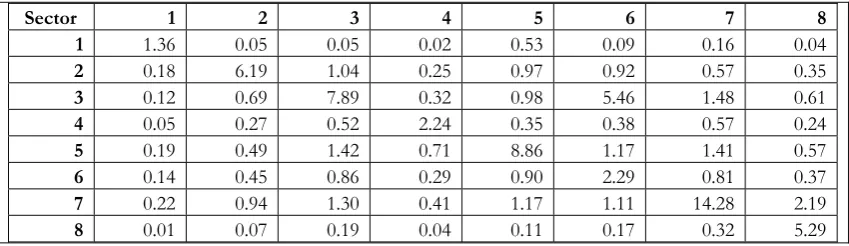
Table A2: Leontief Inverse matrix of the US economy for the year 1995

Sector 1 2 3 4 5 6 7 8

1 1.36 0.05 0.05 0.02 0.53 0.09 0.16 0.04

2 0.18 6.19 1.04 0.25 0.97 0.92 0.57 0.35

3 0.12 0.69 7.89 0.32 0.98 5.46 1.48 0.61

4 0.05 0.27 0.52 2.24 0.35 0.38 0.57 0.24

5 0.19 0.49 1.42 0.71 8.86 1.17 1.41 0.57

6 0.14 0.45 0.86 0.29 0.90 2.29 0.81 0.37

7 0.22 0.94 1.30 0.41 1.17 1.11 14.28 2.19

[image:37.595.86.511.597.720.2]

(38)

[image:38.595.83.515.101.224.2]

Sector 1 2 3 4 5 6 7 8

1 1.32 0.03 0.04 0.02 0.62 0.07 0.11 0.02

2 0.22 6.14 1.06 0.23 0.84 0.84 0.47 0.21

3 0.12 0.45 7.49 0.27 0.85 5.31 0.64 0.23

4 0.03 0.10 0.19 2.13 0.13 0.16 0.15 0.06

5 0.17 0.43 1.29 0.60 8.31 1.01 0.87 0.30

6 0.10 0.37 0.65 0.25 0.67 1.97 0.46 0.15

7 0.28 1.22 1.79 0.56 1.80 1.63 12.87 1.53

[image:38.595.87.513.275.398.2]

8 0.05 0.31 0.44 0.17 0.45 0.40 0.82 4.36

Sector 1 2 3 4 5 6 7 8

1 1.32 0.03 0.04 0.02 0.62 0.08 0.11 0.03

2 0.23 6.37 1.30 0.27 0.95 1.04 0.69 0.33

3 0.10 0.39 7.34 0.25 0.86 5.21 0.72 0.30

4 0.03 0.09 0.20 2.13 0.12 0.17 0.19 0.08

5 0.15 0.37 1.26 0.58 8.07 1.01 1.01 0.43

6 0.08 0.36 0.66 0.26 0.68 1.89 0.59 0.27

7 0.26 1.13 1.61 0.53 1.68 1.46 14.55 2.07

8 0.05 0.34 0.55 0.19 0.50 0.51 1.11 5.58

Table A5: ADF test Sector 1 (Note: + denotes second difference)

Original Variables First Differenced Variables

Variables p-value Stationarity p-value Stationarity

Y1 0.78 No 0 Yes

Y2* 0.86 No 0 Yes

Y3* 0.8 No 0.01 Yes

Y4* 0.83 No 0.02 Yes

Y5* 0.92 No 0.02 Yes

Y6* 0.98 No 0.1 Yes

Y7*+ _{0.86 No} ₀ _Yes

Y8* 0.98 No 0.05 Yes

L1 0.91 No 0 Yes

L2* 0.43 No 0 Yes

L3* 0.84 No 0 Yes

L4* 0.83 No 0 Yes

L5* 0.92 No 0 Yes

L6* 0.96 No 0 Yes

L7* 0.99 No 0.03 Yes

L8* 0.67 No 0 Yes

Credit 0.1 Yes

(39)

[image:39.595.86.513.106.418.2]

Variables p-value Stationarity p-value Stationarity

Y1* 0.7 No 0 Yes

Y2 0.99 No 0.04 Yes

Y3* 0.63 No 0 Yes

Y4* 0.68 No 0 Yes

Y5* 0.99 No 0.02 Yes

Y6* 0.85 No 0 Yes

Y7*+ _{0.99 No} _0.02 _Yes

Y8* 0.91 No 0 Yes

L1* 0.92 No 0 Yes

L2 0.78 No 0 Yes

L3* 0.74 No 0 Yes

L4* 0.67 No 0 Yes

L5* 0.89 No 0.02 Yes

L6* 0.97 No 0.04 Yes

L7* 0.99 No 0.03 Yes

L8* 0.7 No 0 Yes

Credit 0.1 Yes

Trade 0.89 No 0 Yes

Y1* 0.7 No 0 Yes

Y2* 0.99 No 0 Yes

Y3 0.99 No 0.07 Yes

Y4* 0.27 No 0.01 Yes

Y5* 0.91 No 0.05 Yes

Y6* 0.85 No 0 Yes

Y7*+ _{0.99 No} ₀ _Yes

Y8* 0.67 No 0 Yes

L1* 0.87 No 0.01 Yes

L2* 0.89 No 0.04 Yes

L3 0.99 No 0 Yes

L4* 0.26 No 0.02 Yes

L5* 0.48 No 0.01 Yes

L6* 0.93 No 0.02 Yes

L7* 0.99 No 0.03 Yes

[image:39.595.87.514.474.757.2]

(40)

Credit 0.1 Yes

[image:40.595.86.511.76.111.2]

Y1* 0.57 No 0 Yes

Y2* 0.99 No 0 Yes

Y3* 0.6 No 0.01 Yes

Y4+ _{0.99 No} _0.01 _Yes

Y5* 0.59 No 0.01 Yes

Y6* 0.81 No 0.01 Yes

Y7*+ _{0.99 No} ₀ _Yes

Y8* 0.52 No 0 Yes

L1* 0.88 No 0 Yes

L2* 0.93 No 0.01 Yes

L3* 0.58 No 0 Yes

L4 0.98 No 0.04 Yes

L5* 0.82 No 0 Yes

L6* 0.97 No 0.03 Yes

L7* 0.99 No 0.03 Yes

L8* 0.55 No 0 Yes

Credit 0.1 Yes

Variables p-value Stationarity p-value Stationarity

Y1* 0.64 No 0 Yes

Y2* 0.99 No 0 Yes

Y3* 0.84 No 0.01 Yes

Y4*+ _{0.61 No} _0.01 _Yes

Y5* 0.99 No 0.02 Yes

Y6* 0.85 No 0.02 Yes

Y7*+ _{0.99 No} ₀ _Yes

Y8* 0.78 No 0 Yes

L1* 0.88 No 0 Yes

L2* 0.68 No 0.01 Yes

L3* 0.86 No 0 Yes

[image:40.595.87.513.164.483.2]

(41)

L5* 0.95 No 0.04 Yes

L6* 0.85 No 0 Yes

L7* 0.99 No 0.03 Yes

L8* 0.75 No 0 Yes

Credit 0.1 Yes

[image:41.595.83.515.77.172.2]

Y1* 0.95 No 0 Yes

Y2* 0.99 No 0.02 Yes

Y3* 0.83 No 0.02 Yes

Y4* 0.74 No 0 Yes

Y5* 0.99 No 0.02 Yes

Y6+ _{0.99 No} _0.02 _Yes

Y7*+ _{0.99 No} ₀ _Yes

Y8* 0.99 No 0.03 Yes

L1* 0.99 No 0.01 Yes

L2* 0.86 No 0 Yes

L3* 0.95 No 0.01 Yes

L4* 0.85 No 0 Yes

L5* 0.78 No 0 Yes

L6 0.74 No 0 Yes

L7* 0.99 No 0.03 Yes

L8* 0.86 No 0.01 Yes

Credit 0.1 Yes

[image:41.595.87.513.228.548.2]

Variables p-value Stationarity p-value Stationarity

Y1* 0.82 No 0 Yes

Y2* 0.97 No 0 Yes

Y3* 0.99 No 0,09 Yes

Y4* 0.99 No 0,05 Yes

Y5* 0.97 No 0,02 Yes

Y6*+ _{0.99 No} ₀ _Yes

Y7+ _{0.99 No} ₀ _Yes

Y8*+ _{0.99 No} ₀ _Yes

(42)

L2* 0.67 No 0 Yes

L3* 0.94 No 0,01 Yes

L4* 0.92 No 0,01 Yes

L5* 0.82 No 0 Yes

L6* 0.99 No 0,01 Yes

L7 0.99 No 0,03 Yes

L8* 0.29 No 0,01 Yes

Credit 0.1 Yes

[image:42.595.87.514.275.602.2]

Y1* 0.73 No 0 Yes

Y2* 0.99 No 0 Yes

Y3* 0.56 No 0.01 Yes

Y4* 0.26 No 0 Yes

Y5* 0.82 No 0.01 Yes

Y6* 0.98 No 0.03 Yes

Y7*+ _{0.99 No} ₀ _Yes

Y8*+ _{0.99 No} ₀ _Yes

L1* 0.54 No 0 Yes

L2* 0.23 No 0 Yes

L3* 0.31 No 0 Yes

L4* 0.3 No 0 Yes

L5* 0.84 No 0 Yes

L6* 0.56 No 0.04 Yes

L7* 0.99 No 0.03 Yes

L8*+ _{0.99 No} _0.01 _Yes

Credit 0.1 Yes

(43)

[image:43.595.89.510.108.259.2]

Table A13: Matrix Q for US economy for the year 1995

Sector

s 1 2 3 4 5 6 7 8

1 119.14 0.57 -14.71 -8.81 208.63 107.03 71.75 1.89

2 8.10 361.77 61.34 12.97 65.26 125.08 70.09 23.10

3 5.57 11.94 2283.96 36.87 107.24 124.43 1660.22 76.99

4 4.02 5.64 78.71 710.01 50.34 63.89 391.24 36.29

5 5.38 1.96 49.69 42.92 4201.09 31.22 323.00 24.60

6 29.11 20.27 210.50 103.96 336.25 1694.70 1789.44 121.36

7 11.43 12.67 99.72 41.08 100.82 343.09 21769.84 429.05

[image:43.595.83.512.316.467.2]

8 0.02 0.66 20.40 3.39 9.96 21.76 227.25 2436.41

Sector

s 1 2 3 4 5 6 7 8

1 141.85 0.04 -35.90 -22.26 426.81 137.01 47.84 -2.11

2 14.20 498.28 124.65 23.80 87.58 204.53 249.20 50.48

3 10.32 8.94 3601.53 61.45 158.50 179.77 758.83 64.46

4 4.92 3.36 45.71 1223.40 29.96 29.65 273.54 23.39

5 6.85 3.16 96.31 69.36 6539.99 56.71 458.88 35.48

6 28.68 25.63 273.95 182.63 427.18 2321.09 2035.91 125.59

7 17.14 28.98 308.70 115.12 353.68 806.56 39202.54 695.52

[image:43.595.88.510.556.706.2]

8 2.43 5.55 46.91 32.42 69.69 163.60 1304.63 2691.96

Sector

s 1 2 3 4 5 6 7 8

1 187.10 0.51 -63.43 -39.46 674.51 296.24 -37.25 -25.71

2 18.76 748.28 251.14 46.89 146.51 442.32 580.00 83.78

3 10.29 11.42 5905.73 92.61 252.55 310.14 1393.11 131.49

4 5.41 4.01 80.68 2116.26 38.70 48.22 558.65 58.66

5 8.17 4.08 161.22 122.39 9904.94 78.39 966.18 90.77

6 29.24 36.79 467.39 328.61 691.09 3296.05 4550.47 450.53

7 20.77 34.37 265.89 128.83 385.76 990.89 72175.80 1248.84

(44)

[image:44.842.69.776.96.495.2]

Table A16: GVAR Estimation Effects of Foreign Variables on their sector-specific counterparts

Y1 L1 Y2 L2 Y3 L3 Y4 L4 Y5 L5 Y6 L6 Y7 L7 Y8 L8 Y1* -14.59 -68.02 -5.86 22.21 38.17 263.71 -1.34 10.49 -3.68 -453.7 23.8 -70.17 -50.77 -14.47 t-stat -0.57 -2.14* -1.03 0.7 3.64* 1.89* -0.75 0.55 -1.4 -3.57* 1.2 -0.62 -1.27 -0.17 L1* -3.4 -18.5 0.92 27.43 22.9 162.55 0.54 8 -1.77 -241.07 -11.59 25.57 -41.51 -115.45

t-stat -0.36 -1.58 0.23 1.78* 5.11* 2.72* 0.69 1.07 -1.74* -4.92* -2.59* 0.75 -1.51 -2.09* Y2* 7.84 83.5 3.01 6.32 21.48 112.63 9.86 -14.59 1.11 88.42 11.85 25.17 116.59 27.23 t-stat 0.7 1.71* 1.87* 0.71 2.28* 0.9 -1.45 -0.2 0.89 1.48 4.07* 1.34 9.45* 1.1 L2* 3.2 4.83 -1.9 20.72 21.63 117.7 -12.74 54.57 4.56 -560.17 20.03 -13.84 -126.65 -260.9

t-stat 0.4 0.14 -0.46 0.98 1.34 0.54 -1.09 0.44 2.34* -5.06* 3.71* -0.43 -2.99* -3.05* Y3* 4.12 -83.78 -2.95 8.93 65.14 1080.94 49.15 480.62 5.34 1933.26 -14.68 -20.03 386.1 404.18 t-stat 0.37 -2.13* -0.64 1.47 1.77* 2.33* 1.48 1.36 0.46 3.05* -4.46* -0.94 1.84* 1.24 L3* -0.42 6.84 0.71 -1.31 -4.67 -110.98 -14.67 -57.05 -2.68 -342.28 0.11 -3.14 -25.68 -75.82

t-stat -0.36 1.33 0.79 -1.41 -0.97 -1.73* -1.74* -0.57 -1.17 -3.09* 0.22 -0.97 -1.58 -2.32* Y4* -2.35 25.33 -6.04 -4.67 -5.17 109.75 21.17 222.44 -1.46 375.77 -2.75 7.35 48.64 287.05 t-stat -2.11* 5.24* -2.87* -1.78* -1.79* 6.8 1.33 6.16* -2.76* 14.78* -3.04* 1.25 2.44* 7.14* L4* 0.45 -4.33 -0.61 2.32 0.81 -8.32 2.69 -12.12 0.24 -33.5 1.61 -1.26 11.54 -7.02

t-stat 0.66 -1.44 -0.49 1.49 0.91 -1.68* 1.91* -0.81 1.38 -3.89* 5.58* -0.52 2.76* -1.09 Y5* -0.42 4.07 2.17 -2.73 -10.66 38.03 13.42 -13.09 -5.2 -262.43 3.38 23.95 -123.88 -131.49 t-stat -0.38 1.74* 0.6 -0.6 -1.47 1.09 1.91* -0.14 -4.05* -3.98* 1.17 1.28 -3.04* -1.6 L5* 0.03 -0.36 -0.39 -0.45 0.74 2.65 -1.22 23.77 0.5 9.97 -0.58 -1.62 7.77 6.92

t-stat 0.48 -1.22 -0.73 -0.9 1.29 0.82 -1.38 2.13* 3.69* 1.51 -2.11* -0.9 3.5* 1.51 Y6* 0.09 50.1 1.47 -9.85 3.3 -71.82 -8.09 -115.04 -7.18 -76.66 0.92 -1.27 -66.83 -57.98 t-stat 1.12 1.76* 0.29 -1.27 0.35 -1.73* -1.2 -1.14 -0.95 -0.95 2.17* -0.46 -3.82* -1.64* L6* 0.09 -0.77 -0.71 0.17 0.15 0.14 -0.79 0.53 0.11 0.91 0.17 0.27 3.02 -0.98

(45)

Y8* 26.4 -217.92 2.48 27.1 3.78 -27.71 -26.44 -255.7 -39.06 47.87 4.29 306.78 4.45 -8.84 t-stat 1.36 -2.59* 0.29 1.65* 0.45 -0.59 -3.13* -2.27* -1.83* 0.24 1.32 2.01* 2.17* -4.71* L8* -1.48 11.27 0.17 -0.6 -0.22 1.43 1.67 21.1 4.68 8.94 -0.42 -30.5 -0.92 -1.65 t-stat -1.22 2.13* 0.29 -0.66 -0.62 0.7 2.22* 2.09* 1.8* 0.31 -1.5 -2.22* -3.27* -0.91

Trade 0 -0.01 0.01 0.01 0 0 0 -0.01 0 0 -0.01 0.01 -0.01 0 -0.01 0 t-stat 0.48 -4.05* 1.55 2.35* 0.2 -1.12 -1.32 -1.67* 0.45 0.04 -2.77* 2.56* -5.01* -0.08 -3.36* 0.12 Credit 0 0 0 -0.01 0.01 0.01 0 0.01 0 0 0.01 -0.01 0.01 0 0.01 0 t-stat 0.1 0.42 0.36 -2.83* 2.16* 2.16* -0.28 3.22* 0.45 -0.32 4.28* -3.39* 4.22* 0.55 5.01* 0.41

(46)